Article

A Combinatorial Reasoning Mechanism with Topological and Metric Relations for Change Detection in River Planforms: An Application to GlobeLand30’s Water Bodies

1
Applied Technology College, Jilin University, 5372 Nanhu Road, Changchun 130012, China
2
College of Geo-exploration Science and Technology, Jilin University, 938 Ximinzhu Street, Changchun 130026, China
*
Author to whom correspondence should be addressed.
ISPRS Int. J. Geo-Inf. 2017, 6(1), 13; https://0-doi-org.brum.beds.ac.uk/10.3390/ijgi6010013
Submission received: 16 August 2016 / Revised: 5 January 2017 / Accepted: 6 January 2017 / Published: 12 January 2017

Abstract

:
Changes in river plane shapes are called river planform changes (RPCs). Such changes can impact sustainable human development (e.g., human habitations, industrial and agricultural development, and national border security). RPCs can be identified through field surveys—a method that is highly precise but time-consuming, or through remote sensing (RS) and geographic information system (GIS), which are less precise but more efficient. Previous studies that have addressed RPCs often used RS, GIS, or digital elevation models (DEMs) and focused on only one or a few rivers in specific areas with the goal of identifying the reasons underlying these changes. In contrast, in this paper, we developed a combinatorial reasoning mechanism based on topological and metric relations that can be used to classify RPCs. This approach does not require DEMs and can eliminate most false-change information caused by varying river water levels. First, we present GIS models of river planforms based on their natural properties and, then, modify these models into simple GIS river planform models (SGRPMs) using straight lines rather than common lines to facilitate computational and human understanding. Second, we used double straight line 4-intersection models (DSL4IMs) and intersection and difference models (IDMs) of the regions to represent the topological relations between the SGRPMs and used double-start-point 8-distance models (DS8DMs) to express the metric relations between the SGRPMs. Then, we combined topological and metric relations to analyse the changes in the SGRPMs. Finally, to compensate for the complexity of common river planforms in nature, we proposed three segmentation rules to turn common river planforms into SGRPMs and used combinatorial reasoning mechanism tables (CRMTs) to describe the spatial relations among different river planforms. Based on our method, users can describe common river planforms and their changes in detail and confidently reject false changes. Future work should develop a method to automatically or semi-automatically adjust the segmentation rules and the combinatorial reasoning mechanism.

1. Introduction

Rivers are critical for human survival and sustainable development and provide indispensable human resources, such as domestic water, agricultural water, industrial water, shipping, and alluvial plains. However, changes in the river plane shape, called “river planform changes” (RPCs), influence the sustainability of human life, industrial development, agricultural development and national border security. Both extrinsic and intrinsic human activities can affect RPCs. A thorough understanding of a mechanism for detecting RPCs as a fundamental geographical process is critical for predicting river changes that could influence human survival and sustainable development [1,2,3,4,5].
Using remote sensing (RS), geographic data can be rapidly acquired over large areas with high resolution. Using geographic information system (GIS), people can rapidly display, process, and analyse the high volumes of geographic data acquired through RS. Both RS and GIS are increasingly being used to detect and analyse RPCs [6,7,8,9,10,11,12,13,14,15]. To better analyse RPCs, some auxiliary information such as digital elevation models (DEMs), landscapes, and geometries have been applied to the analysis of river planforms. Lau and Franklin (2013) exploited river segment geometries instead of the unreliable or unavailable partial elevation data to generate the induced terrain and the complete river network [16]. Mantilla and Gupta (2005) proposed CUENCAS, which is based on DEMs, to understand river networks [17]. Langhammer and Vilímek (2007) examined the effect of landscape changes caused by floods on the RPCs of the Otava River basin using GIS, RS, and field work [18]. Wohlfart et al. (2016) determined land cover characteristics and dynamics based on optical high-temporal-resolution Moderate Resolution Imagine Spectroradiometer (MODIS) Normalised Differenced Vegetation Index (NDVI) time series for the entire Yellow River Basin. The NDVI changes can be used to analyse hydrological changes [19]. These previous studies—even with some auxiliary information—focused only on the RPCs of a single river or on several rivers within a particular area, identified the changes, analysed the underlying reasons, and described their impacts on humans or other objects. Their results are important for human societies. However, these studies did not propose a method to analyse and classify RPCs in volume by considering their characteristics over large areas or worldwide.
The era of big data has arrived (although no definition of big data has yet achieved consensus among all researchers). However, big data’s characteristics—large volumes, high velocities, wide variety, and huge value but low density—are widely believed to require reforms in data processing [20,21,22,23,24]. Global land cover products are important for analysing global changes in a less-costly and less time-consuming manner, and such products are being developed with increasingly high resolutions. Meanwhile, the data volume continues to increase; when it reaches a certain level, it will be classified as GIS big data. Therefore, it is necessary to develop a method to detect and analyse various RPCs based on their common characteristics. The GlobeLand30 dataset, which is based on the Landsat Thematic Mapper (TM), Enhanced Thematic Mapper Plus (ETM+), and Huan Jing 1 (HJ-1) multispectral images published by China in 2014, includes the highest resolution global land cover products available and was used to obtain the 2000 and 2010 global land cover products, which include water bodies at a resolution of 30 m. These products are freely accessible and available for non-commercial use. Thus, they can serve as a basis for analysing global changes [25,26]. Additionally, GlobeLand30’s accuracy has been validated by many users, and it can be used in most regions of the earth [27,28,29,30]. The 2000 and 2010 water bodies are suitable for obtaining massive initial RPCs through overlay analysis in our study. However, river planforms are dynamic because the river levels change. Thus, dynamic river planforms are temporary and should not be considered as true river planforms; in other words, changes caused by non-normal river levels should be considered as false RPCs. The common approach for detecting RPCs and distinguishing false RPCs is to use a LiDAR-based high-precision DEM at different times; however, this approach is costly on a global scale [31,32,33,34,35,36]. Users can acquire direct RPCs based on RS and GIS data, such as GlobeLand30, but false RPCs are difficult to distinguish automatically from these data because of the lack of DEMs in GlobeLand30.
Spatial relations include topological relations, metric relations, and order relations, and can enhance analyses of both RPCs and false RPCs. Increasingly, studies investigating river planforms have accounted for spatial relations (Peršić and Horvatić (2011) [37], Zhou et al. (2012) [38], Schilling and Jacobson (2012) [39], Hudson et al. (2006) [40], Pan et al. (1999) [41], Hernández-Gracidas et al. (2011) [42] and Buckingham and Whitney (2007) [43]). However, these studies considered only one or a few rivers and, thus, did not express the spatial relations between common river planforms. River planforms are normally expressed as lines or regions in GIS. Therefore, the spatial relations between the river planforms should be considered as spatial relations of lines and regions. Moreover, river planforms must be expressed by lines and regions in organised forms that can be displayed as models in GIS to facilitate human understanding and computer processing. In this paper, considering river planform properties, we develop a reasoning mechanism that combines topological and metric relations to detect and analyse massive amounts of RPCs and distinguish false RPCs.
The remainder of this paper is organised as follows: In Section 2, we discuss related works on the spatial relations of lines or regions. In Section 3, we formalise the river planforms and build their GIS models. In Section 4, we explain the combinatorial reasoning mechanism for RPCs. Finally, in Section 5, we draw some conclusions and discuss future work.

2. Related Works

In this paper, we used a combinatorial reasoning mechanism with topological and metric relations to analyse RPCs expressed as lines and regions; therefore, topological and metric relations and their combinations of lines and regions are important in our study.

2.1. Topological Relations of Lines and Regions

Topological relations can be used to investigate and analyse spatial information between different objects to find those that are invariant under topological transformations such as translation, scaling, rotation and skew. Based purely on topological properties, Egenhofer and Franzosa (1991) proposed a structure that defines the topological relations at a comparatively early time determined by two sets’ four-intersection models [44]. Topological relations are often used to query and analyse spatial relations between simple objects [45,46], and numerous topological relation studies have been conducted to analyse the spatial relations of lines or regions [47,48]. To easily analyse the topological relations between simple objects, researchers have proposed some evolutive topological models based on the four-intersection models. Wang et al. (2014) proposed the DTString topological relation model, which presented the full details of the topological relation between two regions by using a boundary string to resolve the problem that complicated spatial relations could not be differentiated using the currently available models [49]. Gao et al. (2008) developed a model based on point-set topology to demonstrate the topological relations between geometries and directed lines that could serve as a foundation for describing the semantics of the lines compared to the features of the background [50]. However, this model was unable to differentiate insignificant details in the topological relations. Long and Li (2013) developed a formal and complete classification for V9I relations between various types of spatial entities, revealing that the V9I model is, in fact, more expressive than was previously believed [51]. Ber and Napoli (2003) presented a new method that could handle qualitative spatial representations and elucidate the reasons underlying the topological relations based on relation lattices [52]. However, in these previous studies, topological relations served well to resolve the spatial relations between simple regions and lines, but the riverbank lines were too complex to be analysed using existing methods.
To resolve the topological relations between complicated objects, many researchers have studied the topological relations between complicated objects based on the topological relations between simple objects. Deng et al. (2007) proposed a multi-layered method that could describe and determine the complicated topological relations between regions [53]. Schneider and Behr (2005) developed the Proof-By-Constraint-And-Drawing technique, which engendered a variety of exclusive topological relations between different types of complicated spatial data. They demonstrated this method by deriving 43 topological relations between a complex region and a complex line [54]. Renz et al. (2000) made it possible for users to group items by partially lowering the constraints about the shapes of regions [55]. Du et al. (2010) proposed new methods to derive and model the dependences of topological scale relations between multi-scale regions and lines. These dependences of scale were used to derive the topological relations of the lines to differentiate the partitions [56]. Although complex spatial relations between lines and regions can be expressed in terms of topological relations as in the methods developed in these previous studies, the topological relations between riverbank lines remained difficult to describe using their unique planforms.

2.2. Metric Relations of Lines and Regions

Metric relations, often considered to be critical supplements of topological relations, can be divided into direction and distance relations based on quantity or quality. Guo and Du (2009) presented computational methods to derive topological relations from direction relations that could produce topological information in cases where topological relations are not available. These methods were expected to give relatively precise results [57]. Wang (2014) proposed a novel model called the Radial model that could handle both qualitative and quantitative direction relations and was based on the principle of rays transmitted as straight lines [58]. Deng and Li (2007) proposed a statistical modelling method for the directional relations of spatial objects that could describe such a relation more accurately than previous methods because it did not require approximating the objects [59]. Lin et al. (2013) proposed an undirected straight line graph called a constrained Delaunay (CD) graph to represent spatial adjacency and spatial neighbourhood relations with both obstacle and facilitator constraints in the real world [60]. However, these studies are critical for analysing spatial relations between objects, but considered only normal lines or regions and, thus, were not suitable for detecting RPCs.

2.3. Topological and Metric Combined Relations of Lines and Regions

To resolve the shortcomings of topological and metric relations, researchers have analysed the combinational topological and metric relations between lines and regions. Du et al. (2012) presented a generic application example using case-based reasoning (CBR) to cope with geographic problems. To better understand spatial relations, a new element of the “Geographic Environment” was incorporated into the standard CBR case representation model [61]. Nedas et al. (2007) extended the nine-intersection model by focusing on the metric details of the relations between lines via the ratio split and measures of closeness, which can help to obtain additional details about the comparative geometry and positioning of objects [62]. Xu (2007) developed an approach using quantitative values in which the metric and topological indices can both be used to better formalise the natural-language spatial predicates compared to those obtained using the topological indices only [63]. Legleiter (2014) presented geostatistical models that were sensitive to changes in terms of the shape, size and orientation of the channel features instead of a simple translation of the morphology. These results highlight the significance of considering the transverse and streamwise components jointly rather than singly [64]. These studies are more useful for detecting the changes of spatial objects than are separate topological or metric relations. However, a targeted method for change detection in and analysis of common river planforms has not been developed previously. Therefore, models of river planforms should be constructed to detect RPCs using combined reasoning based on topological and metric relations.

3. River Planforms and Their GIS Models

River planforms on earth are so complicated and diversiform that each river has a unique planform. However, commonalities exist among the different river planforms. To detect RPCs, river planforms must be classified based on their common characteristics to build GIS models.

3.1. Two Typical Classifications of River Planforms

Brice (1983) and Fuller (2007) presented two typical classifications for river planforms. Brice classified river planforms into sinuous canaliform, sinuous point bar, sinuous braided, and nonsinuous braided types, as illustrated in Figure 1, whereas Fuller classified river planforms by their degrees of sinuosity, braiding and anabranching, as illustrated in Figure 2 [65,66].

3.2. GIS Models of River Planforms

However, these two typical classification systems for river planforms are difficult to use to represent all river planforms on earth. Taking these typical classifications into account and considering the river planforms found in nature, we classified river planforms into simple nonsinuous (nonsinuous without braidings or anabranchings), nonsinuous braided, nonsinuous anabranched, simple sinuous (sinuous without braidings or anabranchings), sinuous braided, and sinuous anabranched planforms. In this paper, we used lines and regions to express the river planforms in GIS: Bank lines were expressed by lines, while braidings or anabranchings were expressed by regions. To perfect our classified river planforms, two special conditions must be considered: The first such condition is that it is difficult to distinguish between braidings and anabranchings, which are both expressed by regions in GIS. The second special condition is that when the width of a river is too small to be expressed by double lines or a branding on a specified scale in GIS, the river planform must be expressed by a single line. Based on the two typical river planform classifications and two special conditions presented above, river planforms can be expressed using five types of GIS models—single line, double line, double line with one internal region, double line with several internal regions, and three or more lines with several regions—as illustrated in Figure 3. Figure 3a shows a river planform with a width so small that it had to be expressed by a single line. Figure 3b presents simple nonsinuous and simple sinuous planforms expressed using a double-line model; Figure 3c depicts a model with double lines containing one region used to express nonsinuous and sinuous planforms with one central bar. Figure 3d shows nonsinuous and sinuous braided or anabranched planforms expressed as double lines with several regions. Finally, Figure 3e displays three or more lines with several regions used to depict complicated nonsinuous and sinuous braided or anabranched planforms. The lines consist of two endpoints (a start point [SP] and endpoint [EP]) and an interior, and the regions consist of a boundary (H-boundary) and an interior (H-interior).

3.3. Simple GIS Models of River Planforms

To perfect the GIS models of the river planforms, we used straight lines instead of common lines to facilitate human understanding and computational analysis. This choice did not impact the topological relations of the river planforms. Moreover, complicated nonsinuous and sinuous planforms expressed by three or more lines with several regions can be subdivided into several other simpler GIS models, such as the double-line model and the double-line one-region model. Hence, we did not include this model in the simple GIS river planform models (SGRPMs). The SGRPMs, which comprise single straight line (SSL) models (SSLMs), double straight line (DSL) models (DSLMs), DSL one-region models (DSL-1RMs), and DSL several-regions models (DSL-SRMs), are illustrated in Figure 4. DSL-SRMs could be considered as the most integrated models of SGRPMs (To express DSL-SRMs simply, we use two regions that represent several regions belonging to them). When the regions change into one, they become DSL-1RMs and when regions disappear, they become DSLMs—in other words, the DSLM can be considered as a DSL with an empty set (for the disappeared region). When the river width is too small to be depicted, DSLMs become SSLMs—in other words, SSLMs are the simplest, and an SSLM should be considered as a special DSLM that consists of an SSL and an empty set (for another SSL) with an empty set (for the disappeared region). Figure 4a–d show an SSLM, a DSLM, a DSL-1RM, and DSL-SRM, respectively.

4. Combinatorial Reasoning Mechanism for RPCs

RPCs can be expressed based on their spatial relations, but it is difficult to distinguish RPCs solely in terms of their topological or metric relations. In this paper, the spatial relations between river planforms or SGRPMs consist of topological and metric relations and their combinations to fully express RPCs. The spatial relations between SGRPMs constitute the foundation for the spatial relations between the river planforms, and complex river planforms are expressed by the combination of several SGRPMs. Based on the characteristics and GIS expressions of river planforms, we have proposed segmentation rules that can be used to divide an entire river planform into several SGRPMs and, thus, more readily analyse the spatial relations between river planforms and describe the RPCs.

4.1. Spatial Relations between SGRPMs

The spatial relation between an SSLM at Time 1 and a DSLM at Time 2 is different than that between a DSLM at Time 1 and an SSLM at Time 2. However, the reasoning mechanisms, which are based on the spatial relations involving the resulting changed river planforms, remain the same. Hence, we considered these two types of spatial relations to be equivalent. Based on the analysis presented above, we divided the spatial relations into several types, as shown in Table 1.
Before analysing the topological relations between SGRPMs, those with a low probability and that are unlikely to be representative must be excluded to make the remaining relations simple and effective. Because river planforms are dynamic and bank lines are always continuous, the topological relations between bank lines should be considered as topological relations between straight lines, which can extend or shorten to some extent. In other words, the topological relations between bank straight lines will not change if the lines change in length to a certain extent. We defined a true topological relation between straight lines as one that does not change when the lines are extended or shortened by an arbitrarily small amount. In contrast, relations that do change are called false spatial relations. Figure 5a illustrates the topological relation between Straight line A at Time 1 and Straight line α at Time 2 when Straight line A is shortened by an arbitrarily small amount, such as ε 1 and ε 2 , based on the two endpoints, and Straight line α   changes by the same amount as Straight line A ( δ 1 and   δ 2 , respectively). Figure 5b–d illustrate the same situation as Figure 5a. Figure 5e depicts the topological relation between Straight line A and Straight line α when Straight line A is extended by an arbitrarily small amount based on the two endpoints, and Straight line α changes by the same amount as Straight line A. Figure 5f–h show the same situation as Figure 5e. The topological relations illustrated in Figure 5a,e are the same, and they remain the same after shortening or extending. We call this type of topological relation the true topological relation between the SGRPMs. By the same reasoning, we call the topological relations illustrated in Figure 5b,f true topological relations, and Figure 5c,g are the same as Figure 5b,f. In contrast, although the topological relations illustrated in Figure 5d,h are the same, because they differentiated into two different types of spatial relations after shortening or extending, they present false topological relations between the SGRPMs, and, in this paper, we eliminate them from the topological relations between SGRPMs. Moreover, Figure 5 illustrates only the topological relations between SSLs at different times. It is important to note that a straight line can be considered a model of a bank line from the DSLM. However, topological relations between two DSLs at different times must conform to the same rule, as addressed for SSLs above.

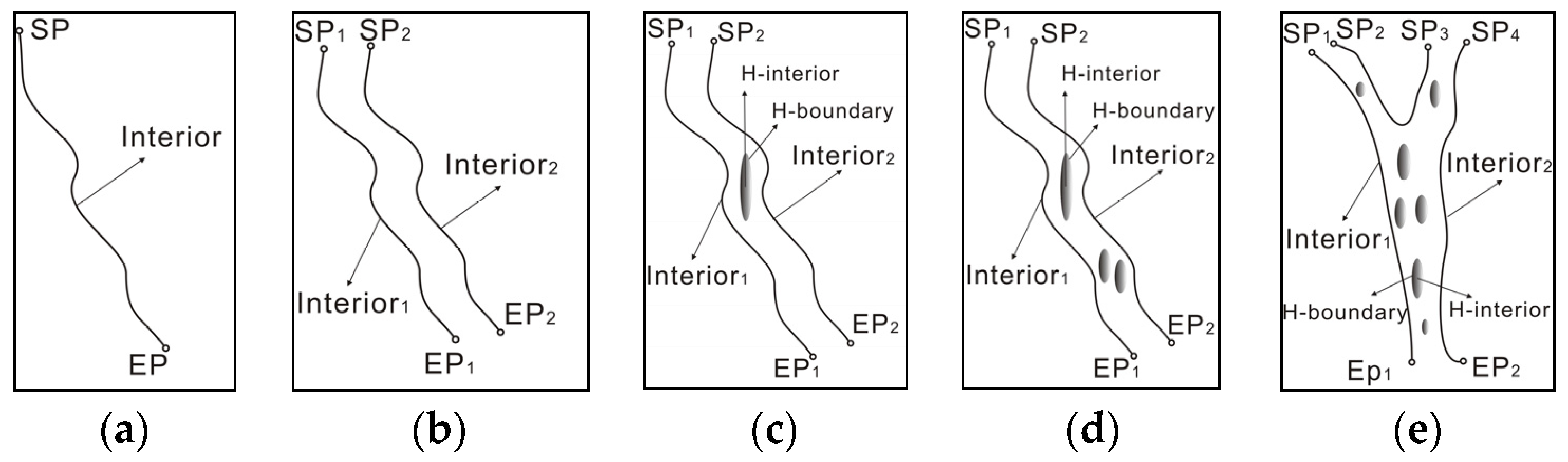
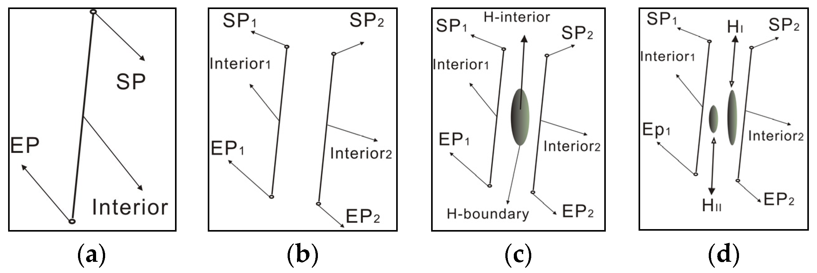
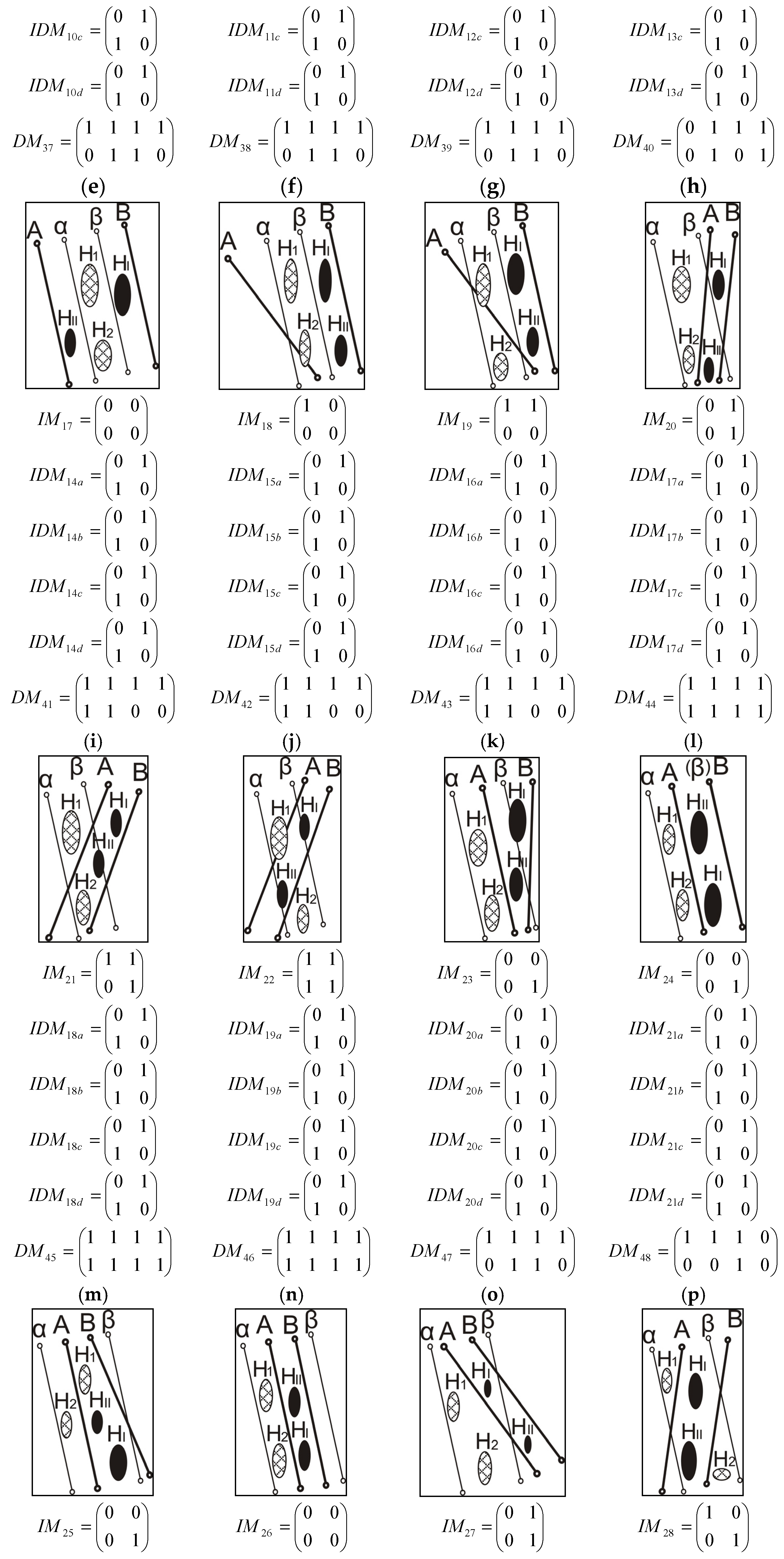
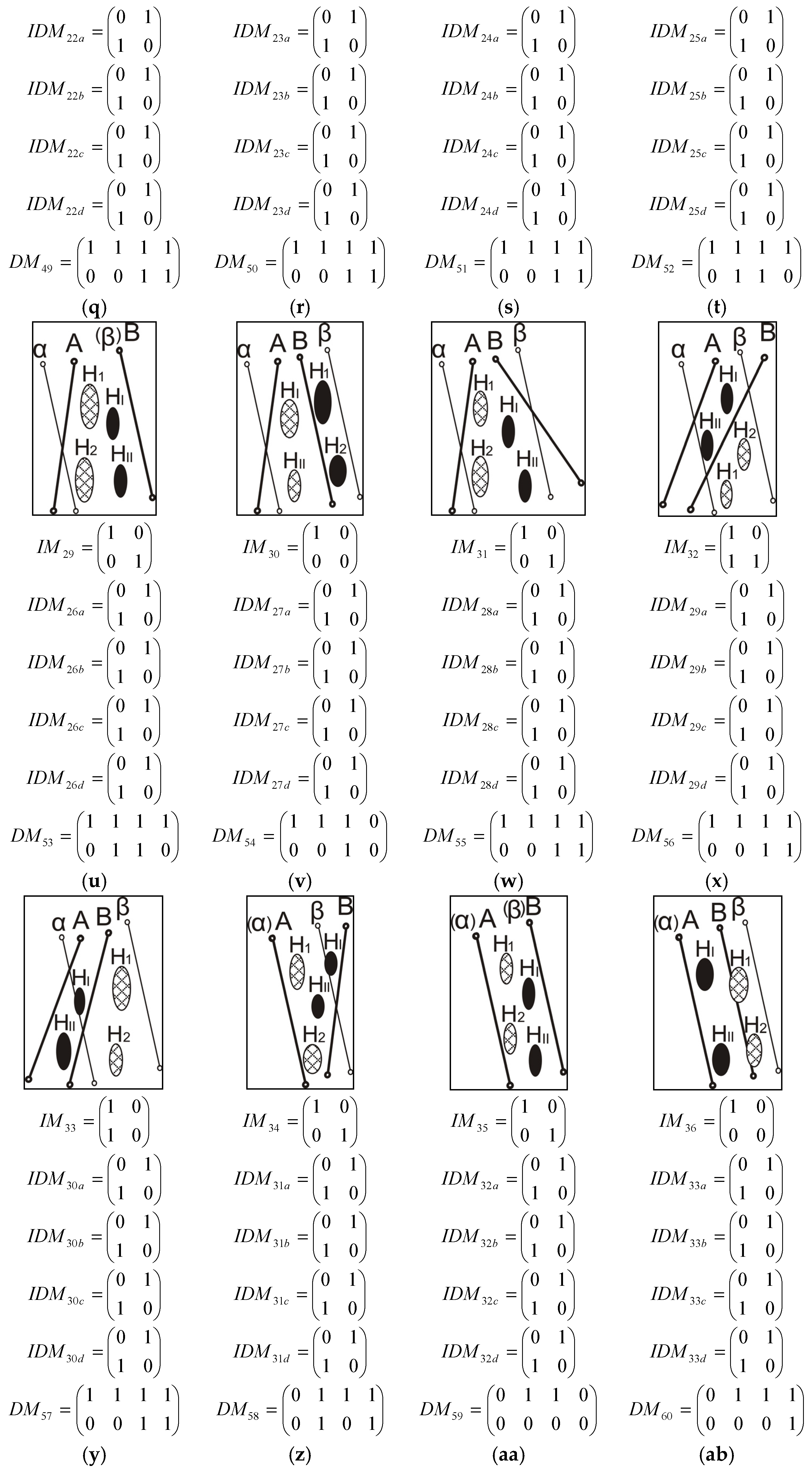
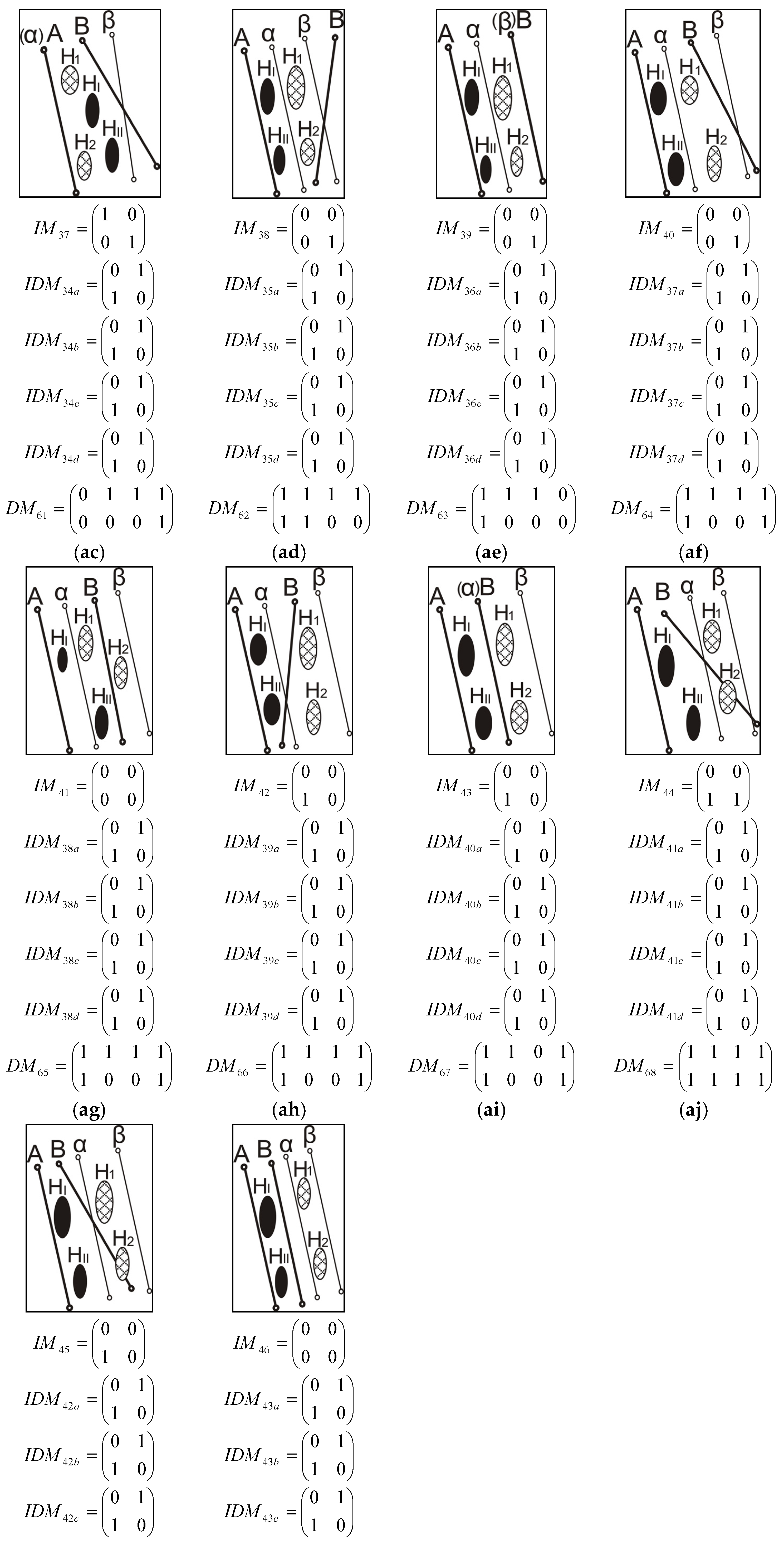
4.1.1. Topological Relations between SGRPMs

Topological relations between SGRPMs should be expressed as topological relations between DSLs and between their regions. We proposed a DSL 4-intersection model (DSL4IM) based on the four possible intersections of the interiors ( A o , B o ) of the DSL at Time 1 with the corresponding components of the DSL at Time 2 to express the topological relations between the two DSLs of SGRPMs at different times. The DSL4IM, which expresses the topological relations between Straight line A (right) and Straight line B (left) at Time 1 and Straight line α (right) and straight line β (left) at Time 2, is characterised by a binary value (empty (0), non-empty (1)) of the set intersections of A’s interior and B’s interior with α ’s interior and β ’s interior (Equation (1)). In particular, the DSL4IM between two SSLMs can be considered as the intersections of A’s interior and one empty set with α ’s interior and one empty set:
I ( A , B , α , β ) = ( A ° α ° A ° β ° B ° α ° B ° β ° ) .
The topological relations between regions are important supplementary conditions when the topological relations between two DSLs (or SSLs) are insufficient to distinguish between true and false RPCs. We used the intersection and difference model (IDM) proposed by Deng et al. (2007) [53] to express the topological relations between regions. This model can more accurately describe the topological relations between a region and an empty set than can other models. The topological relations between regions based on IDM can be represented by Equation (2):
I D ( H I , H 1 ) = ( H I ° H 1 ° H I H 1 H 1 H I H I H 1 ) ,
where H I o H 1 o and H I H 1 represent the intersections between H 1 s interior ( H I o ) and H 1 s interior ( H 1 o ) and between H 1 s boundary ( H I ) and H 1 s boundary ( H 1 ), respectively; and H I H 1   and H 1 H I represent the differences between regions H I (bounded by A and B) and H 1 (bounded by α and β ). We can describe these using one typical model when changes can be detected only by the topological relations between two DSLs. Moreover, they can be fully described when the changes are not fixed by using only the topological relations between two DSLs. However, the topological relations between one or more pairs of regions should be expressed by one or more topological relation matrixes.
The topological relations between DSLs (or SSLs) and regions are not described in this paper because they are complicated and unnecessary. Moreover, the topological relations between DSLs and between regions are sufficient to depict RPCs.
Because the DSL-SRM is the most integrated model of SGRPMs, all the topological relations between SGRPMs can be considered as between DSL-SRMs or changed DSL-SRMs. In this paper, each topological relation between two DSL-SRMs is expressed by one DSL4IM (IM) and four IDMs of regions. To simplify understanding this concept, we describe one typical topological relation between two DSL-SRMs and their matrixes (IM for DSL4IM; IDM a , IDM a , IDM c and IDM d for the IDM of regions; IDM a in relation to H I and H 1 , IDM b in relation to H I and H 2 ; IDM c in relation to H II and H 1 ; and IDM d in relation to H II and H 2 ) are shown in Figure 6.
When the topological relations change between the DSL-1RM and the DSL-SRM, there will be one IM and two IDMs ( IDM a and IDM b ); when the topological relations change between the DSL-1RM and the DSL-1RM, there will be on IM and one IDM ( IDM a ); when the topological relations change between the DSLM and the DSL-SRM, there will be one IM and two IDMs ( IDM a and IDM b , expressing an empty set with H 1 and an empty set with H 2 ); when between the SSLM and the DSL-SRM, there will be one IM and two IDMs (( IDM a and IDM b , expressing an empty set with H 1 and an empty set with H 2 ), and so on. Finally, the topological relations change between the SSLM and the SSLM, there will be only one DSL4IM.

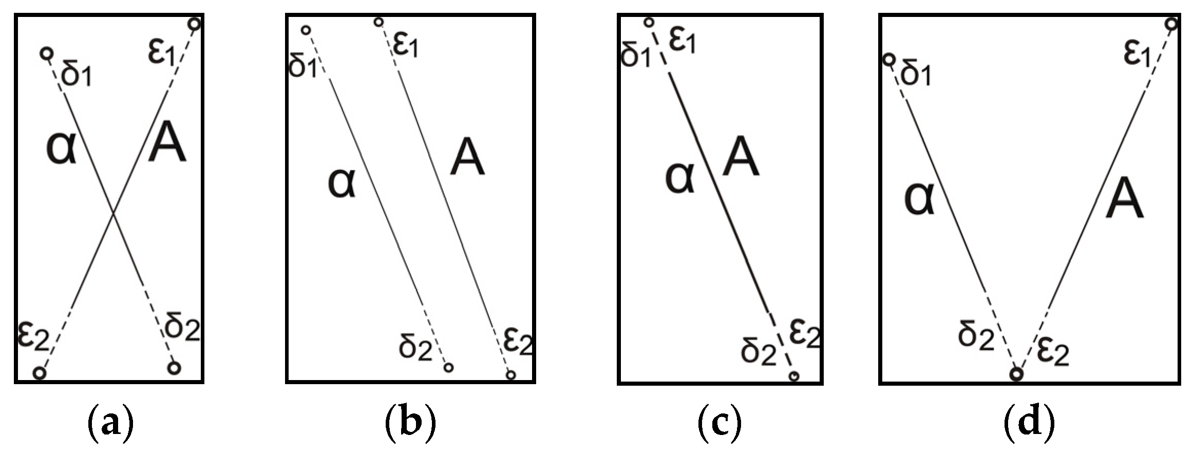
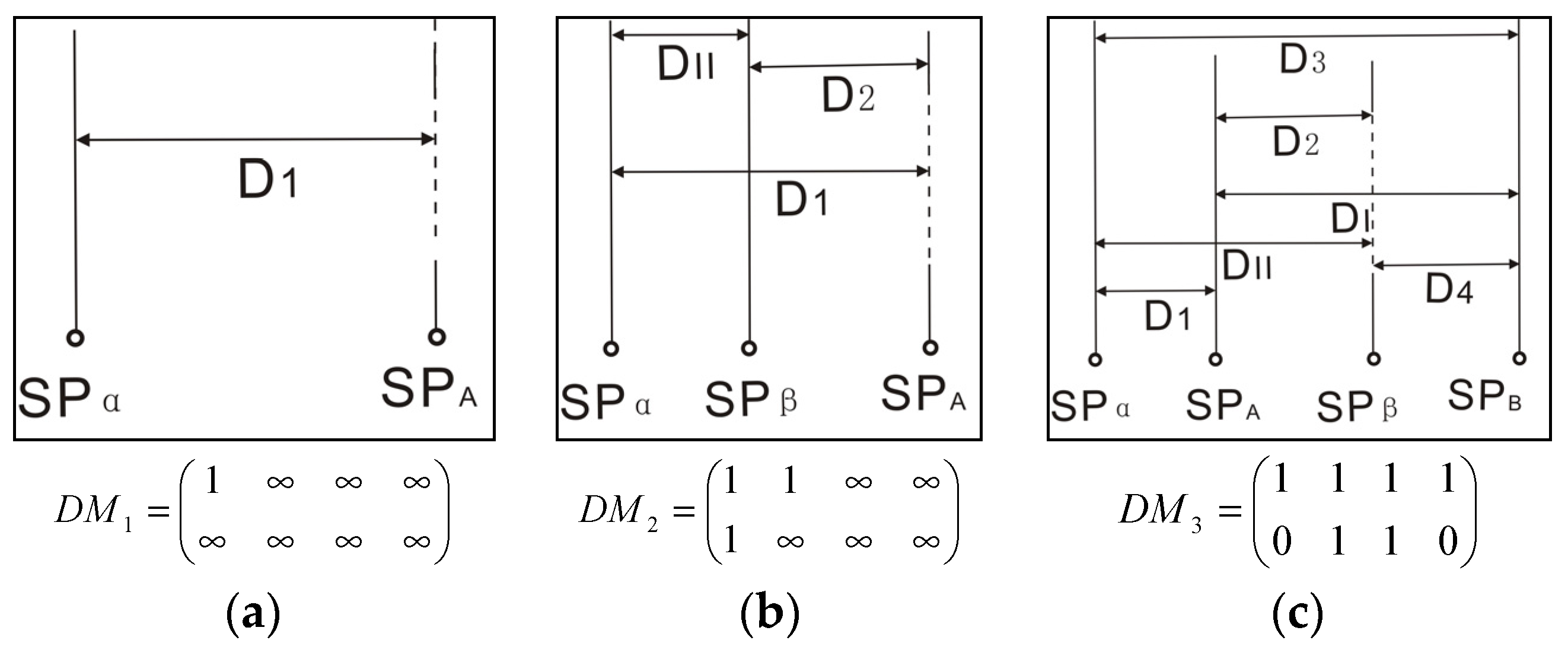
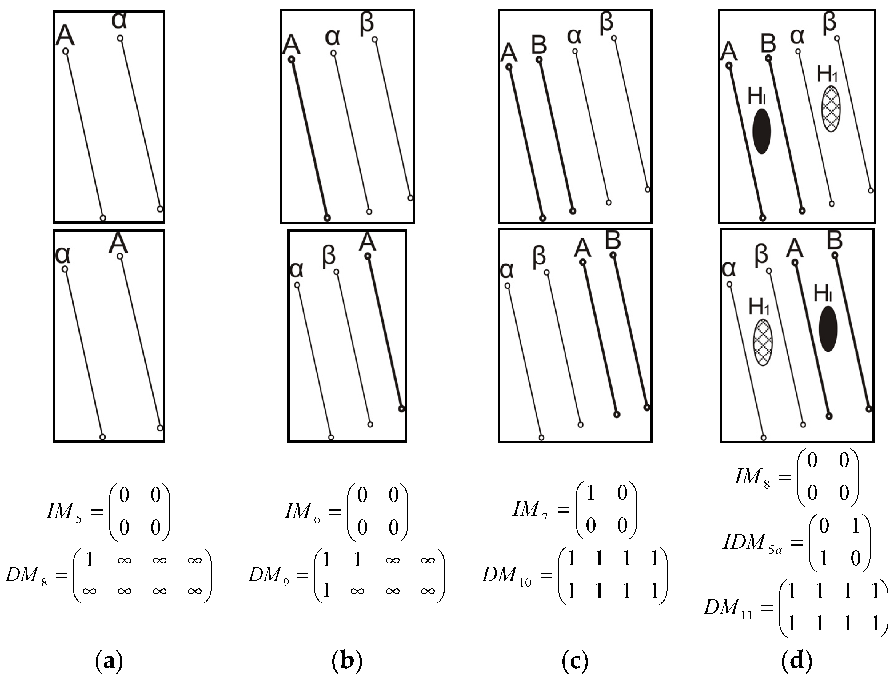
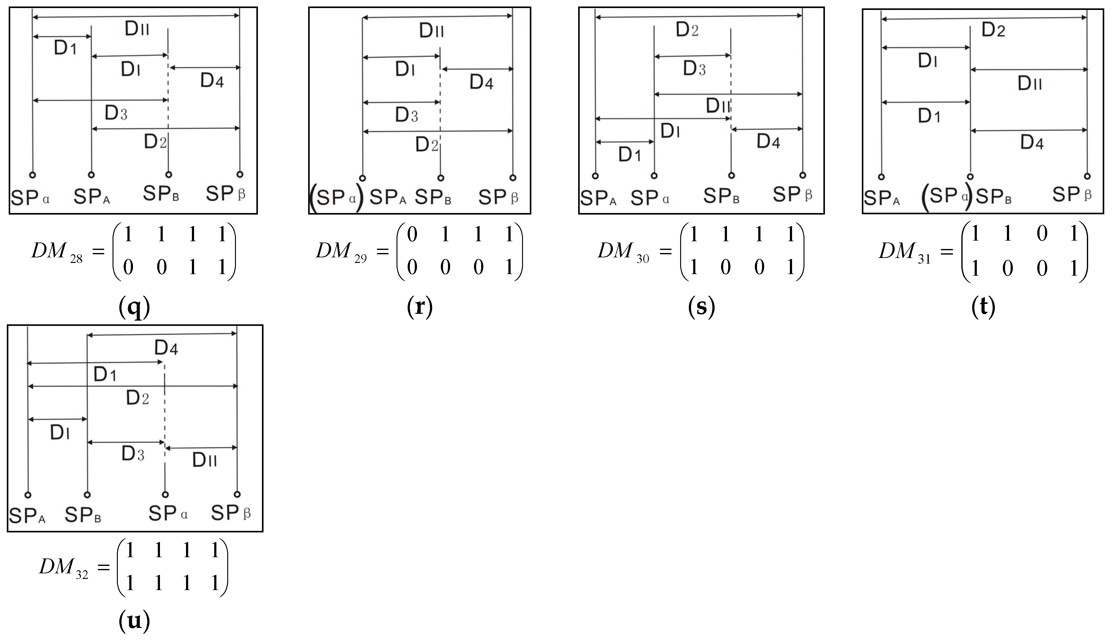
4.1.2. Metric Relations between SGRPMs

We propose a double-start-point 8-distance model (DS8DM) that expresses the metric relations between DSL A and B and between DSL α and β   that is characterised by three distance values (0, 1, ): between A’s SP and B’s SP and between α ’s SP and   β ’s SP (Equation (3)):
D ( A , B , α , β ) = ( D 1 D 2 D 3 D 4 D D 1 D D 2 D D 3 D D 4 ) ,
where
  • D 1 is the distance between A’s SP ( SP A ) and   α ’s SP ( SP α );
  • D 2 is the distance between A’s SP ( SP A ) and β ’s SP ( SP β );
  • D 3 is the distance between B’s SP ( SP B ) and α ’s SP ( SP α );
  • D 4 is the distance between B’s SP ( SP B ) and β ’s SP ( SP β );
  • D I is the distance between A’s SP ( SP A ) and B’s SP ( SP B ); and
  • D II is the distance between   α ’s SP ( SP α ) and   β ’s SP ( SP β ):
  • DD 1 = D 1 + D 2 D II ;
  • DD 2 = D 3 + D 4 D II ;
  • DD 3 = D 1 + D 3 D I ; and
  • DD 4 = D 2 + D 4 D I .
Moreover, the distance value (0) indicates that the distance is 0, the distance between an SP and an empty set is defined as , and the distance value (1) denotes that the distance is not 0 and . Then, the values representing the DS8DM can be described as follows:
If the values of D 1 , D 2 , D 3 , and D 4 are 0, then the two SPs are equal;
If the values of D 1 , D 2 , D 3 , and D 4 are 1, then the two SPs are disjoint;
If the values of D 1 , D 2 , D 3 , and D 4 are , then at least one SP does not exist, and the values of the corresponding elements such as DD 1 , DD 2 , DD 3 , and DD 4 should not be calculated. That is, if the value of D 1 is , DD 1 and DD 3 should not be calculated; instead, they should just be defined as .
If the value of DD 1 is 0, then SP A is between SP α and SP β , or SP A equals SP α or SP β . If the value of DD 1 is 1, then SP A is outside SP α and SP β .
If the value of DD 2 is 0, then SP B is between SP α and SP β , and if the value of DD 2 is 1, then SP B is outside SP α and SP β .
If the value of DD 3 is 0, then SP α is between SP A and SP B , and if the value of DD 3 is 1, then SP α is outside SP A and SP B .
If the value of DD 4 is 0, then SP β is between SP A and SP B , and if the value of DD 4 is 1, then SP β is outside SP A and SP B .
All the DS8DMs of SGRPMs can be classified into three types that describe SSLs at Time 1 and SSLs at Time 2, SSLs at Time 1 and DSLs at Time 2, and DSLs at Time 1 and DSLs at Time 2. DS8DMs of DSLs at Time 1 and DSLs at Time 2 can be considered the most integrated types, while the other two types can be considered as DS8DMs of changed DSLs at Time 1 and changed DSLs at Time 2. We express the DS8DMs by three typical situations: between two SSLs (Figure 7a), between one SSL and one DSL (Figure 7b), and between two DSLs (Figure 7c).
For a thorough understanding of the metric relations between SGRPMs, we list all 21 DS8DMs in Figure A1 in the Appendix A.

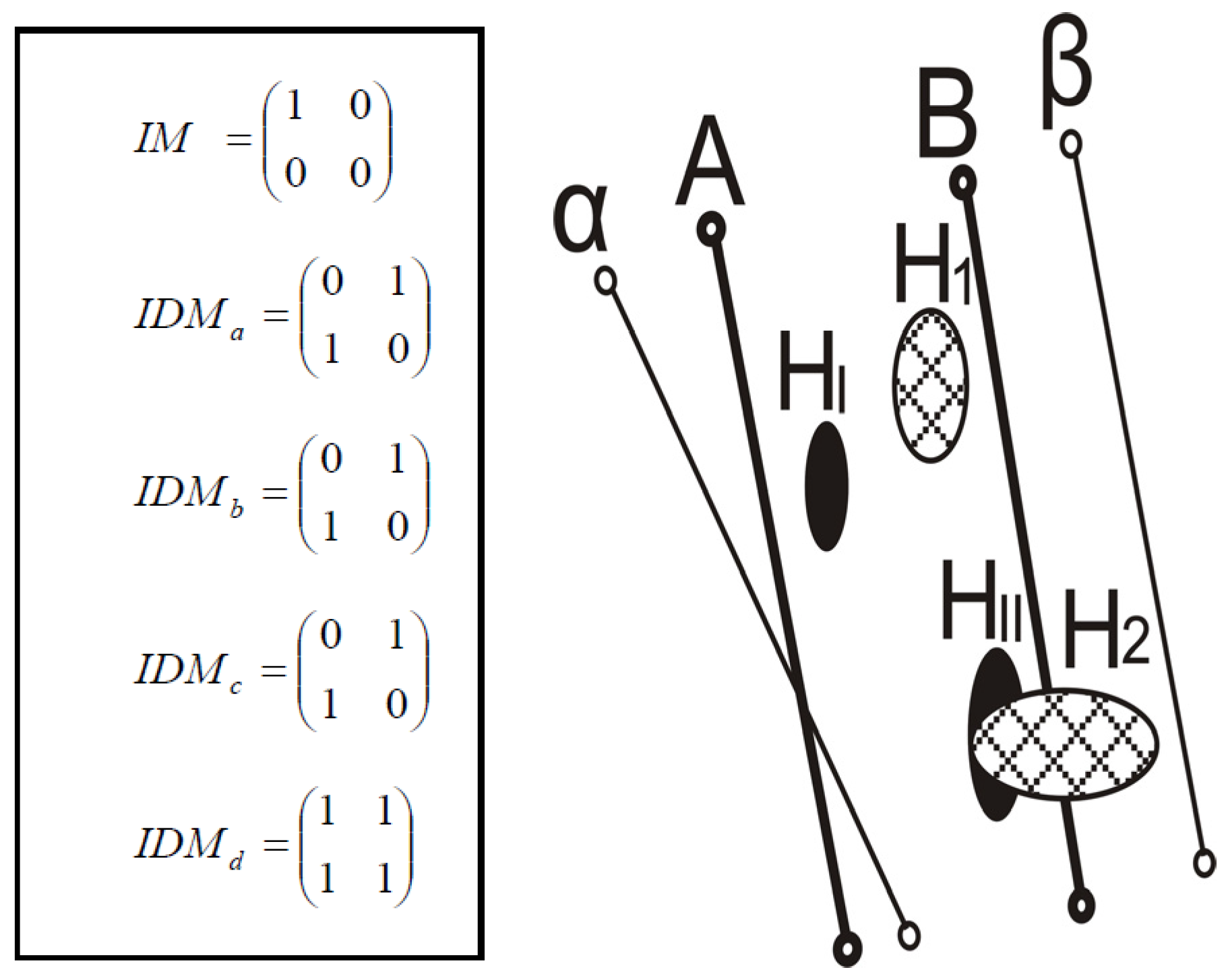
4.1.3. Combinatorial Reasoning Mechanism with Topological and Metric Relations between the SGRPMs

Because of the limitations of expressing a change between SGRPMs using only topological or metric relations, we propose a combinatorial reasoning mechanism involving both topological and metric relations. This combination contains the matrixes of DSL4IMs and the IDM of regions and DS8DMs. To express the combinatorial reasoning mechanism thoroughly, we propose four similar situations between SGRPMs (which are easy to confuse) to explain how it works to distinguish different changes. To distinguish between the first situation (Figure 8a) and the second situation (Figure 8b), which have the same DSL4IMs and IDMs, the DS8DM is critical. To distinguish between the second situation (Figure 8b) and the third situation (Figure 8c), which have the same DS8DM and IDMs, the DSL4IM is critical. To distinguish between the third situation (Figure 8c) and the fourth situation (Figure 8d), which have the same DSL4IM and IDMs, the DS8DMs are critical. Based on these combinatorial reasoning matrixes, we can distinguish the different types of changes between the SGRPMs except for changes between whole left migrations and whole right migrations, which result in the same matrixes, as shown in Figure 9. However, these four similar situations do not comprise all the situations between whole left migrations and whole right migrations. Because IDMs are useless in these situations, RPCs with the same bank line situations—as shown in Figure 9—are all true changes, and they can be further differentiated based on context. Hence, using the combinatorial reasoning mechanism we can eliminate most false changes caused by bank lines widening or narrowing (Figure 8b is probably a false change caused by bank lines widening from Time 1 to Time 2).
For a thorough understanding of the combinatorial reasoning mechanism, combined topological and metric relations between SGRPMs are needed. In particular, those between DSL-SRMs are essential. Considering that the IDMs between two regions are of eight types (disjoint, meet, overlap, cover, contain, coveredby, containedby, and equal) [53], listing all the situations is too complex. Consequently, Figure A2 in the Appendix A lists just 38 typical relations between two DSL-SRMs that express only one typical topological relation between regions.

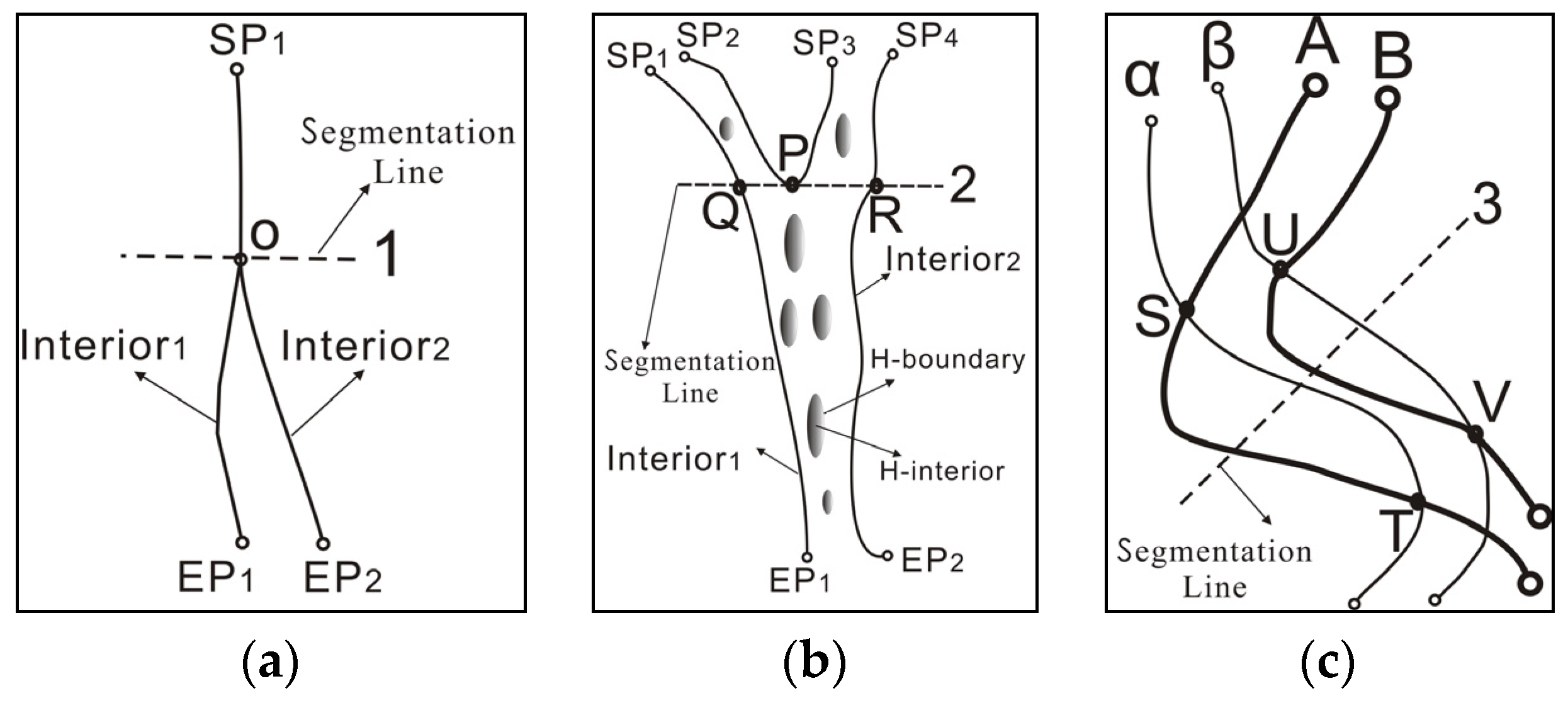
4.2. Segmentation Rules for River Planforms

Common river planforms are always too complicated to be expressed by a single SGRPM. Hence, it is necessary to segment common river planforms into several SGRPMs. We proposed three segmentation rules for segmenting a common river planform into several SGRPMs, which are described as follows.
Segmentation Rule 1: If a river planform changes from an SSLM to a DSLM, or vice versa, it will be segmented by segmentation line 1, which passes through the change point O (Figure 10a); thus, the river planform will be segmented into a DSLM and an SSLM.
Segmentation Rule 2: If the bank lines of a river planform change from double line to three or more lines, or vice versa, it will be segmented by segmentation line 2, which passes through the change point P, an arbitrary internal point Q for the right line and an arbitrary internal point R for the left line (Figure 10b); thus, the river planform will be segmented into DSLMs, DSL-1RMs, and DSL-SRMs.
Segmentation Rule 3: If a river planform at Time 1 intersects with a river planform at Time 2 and two or more intersection points exist between any of the bank lines, it will be segmented by segmentation line 3, which passes through an arbitrary point between the neighbouring intersection points of the bank lines such as U and V or S and T (Figure 10c); thus, the river planforms at Time 1 and Time 2 will be segmented into two or more DSLMs, DSL-1RMs, and DSL-SRMs. These three segmentation rules must be considered together; therefore, if a river planform satisfies all three rules, it must be segmented by all three.
Based on these segmentation rules, we used six segmentation lines to segment a practical river planform into several parts that can be simplified to SGRPMs as illustrated in Figure 11. H I H VIII are regions of the river planform at Time 1, and points A, B, C, D, E, and F are the SPs or EPs at Time 1. H 1 H 9 are regions of the river planform at Time 2, and points α, β, γ, δ, ε, and ζ are the SPs or EPs at Time 2.

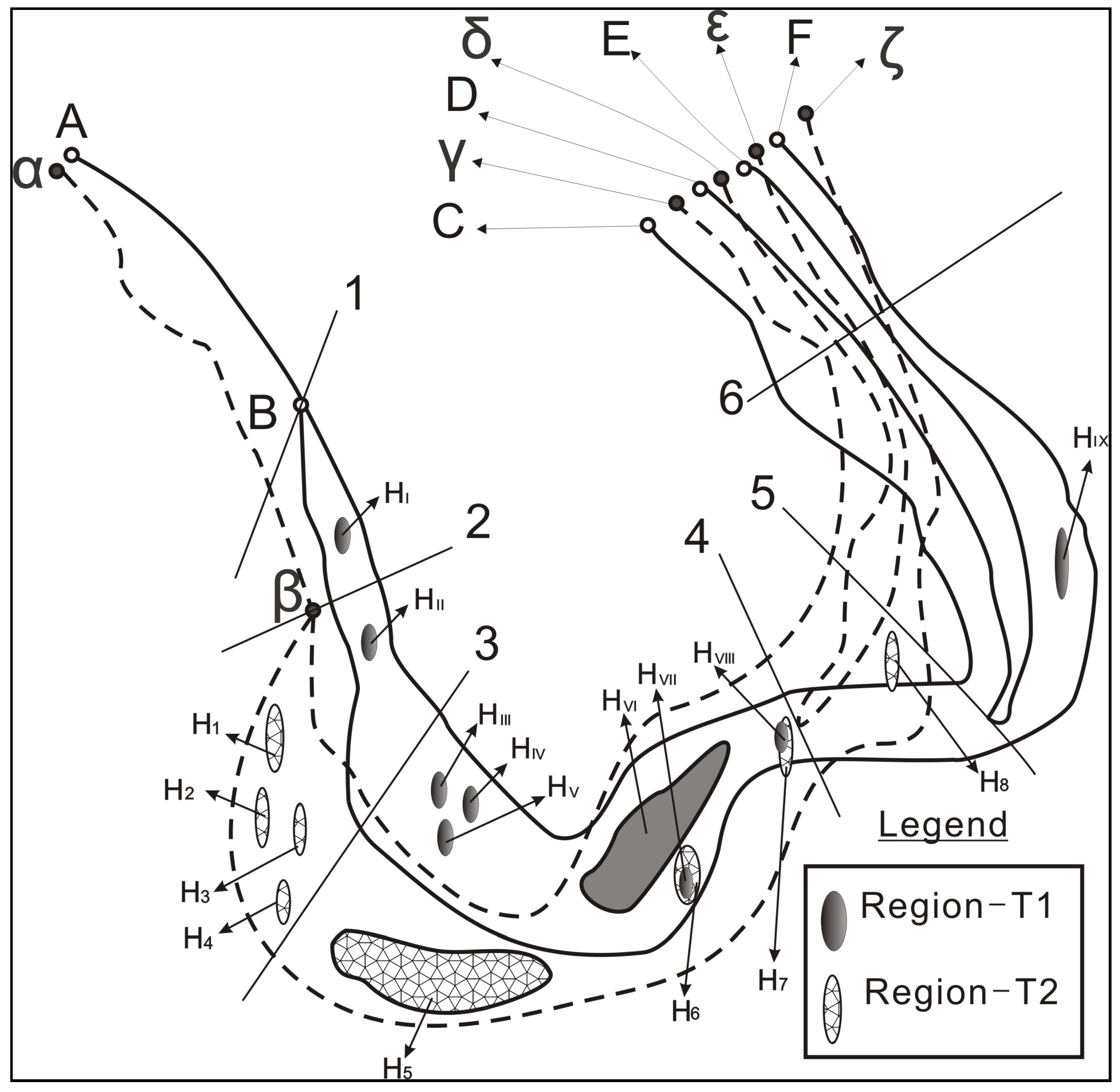
4.3. A Combinatorial Reasoning Mechanism Table of River Planforms

Because of the complexity of the river planforms, based on the combinatorial reasoning mechanism between the SGRPMs and segmentation rules, we present a combinatorial reasoning mechanism table (CRMT) to describe the combinatorial reasoning mechanism for RPCs in detail. The CRMT consists of several DSL4IMs, IDMs of regions, and DS8DMs of the corresponding SGRPMs, as illustrated in Table 2. Considering the context, people using the CRMT can express all RPCs—including whole right migrations and whole left migration that have the same combined topological and metric matrixes by the context. Moreover, the change processes that are important for analysing river planforms can be analysed by the CRMT. To simply and clearly describe the IDMs and DSL4IMs, we used subscripts to represent the corresponding relations and distinguish between the matrixes with the same values, i.e., ( 0 1 1 0 ) ~ H 6 H III VI , VIII represents the IDMs between H 6 and H III to H VI and H VIII , which can all be described by the same matrix ( 0 1 1 0 ) . We used the corresponding points to distinguish between different DSL4IMs and DS8DMs; for instance, ( 0 0 1 0 ) ~ F , C δ , γ from Segments L4–L5 represents the DSL4IMs between the river planforms at Time 1 and Time 2, in which the bank lines contain points F and C. Here, δ , γ should be represented by ( 0 0 1 0 ) , and its corresponding DS8DMs should be represented by ( 1 1 1 0 1 1 0 1 ) .

5. Conclusions and Future Work

This paper proposes a combinatorial reasoning mechanism that utilises topological and metric relations to describe the spatial relations between river planforms for detecting RPCs and to distinguish between true and false RPCs. Five types of GIS models are developed based on natural river planforms and two typical river planform classifications. Four types of SGRPMs are presented based on GIS models of the river planforms to describe the topological relations between them. The DSL4IMs are provided to describe the topological relations between straight lines, the IDMs of regions are developed to express the topological relations between regions, and the DS8DMs are proposed to determine the metric relations between straight lines. Three segmentation rules are developed to segment the river planforms into the SGRPMs. A practical river planform is analysed by the CRMT, which can describe the combinatorial reasoning mechanism of whole river planforms.
The proposed reasoning mechanism can be used to detect RPCs, identify false changes and describe the change processes for massive river planforms. Developing a method to automatically or semi-automatically adjust the reasoning mechanism should be the focus of future research.

Acknowledgments

The authors are grateful to Jun Chen of the National Geomatics Centre of China (NGCC) for his valuable suggestions on change detection of GlobeLand30’s Water Bodies. The authors would like to sincerely thank the reviewers and editors for their thoughtful comments and suggestions improved the quality of this paper. The authors thank American Journal Experts (AJE) for English language editing.

Author Contributions

Liang Leng and Shengbo Chen designed the framework of this paper. Liang Leng drafted and finalized the manuscript. Guodong Yang analysed and verified the combinatorial reasoning mechanism. Shengbo Chen contributed to the structuring of the text. All authors revised the paper together and have read and approved the final manuscript.

Conflicts of Interest

The authors declare no conflict of interest.

Appendix A

Figure A1. The DS8DMs between the SGRPMs. (a)–(u) depict the 21 DS8DMs between the SGRPMs.
Ijgi 06 00013 g012aIjgi 06 00013 g012b
Figure A2. Combinatorial reasoning mechanism with topological and metric relations between the SGRPMs. (a)–(al) depict 38 typical relations between two DSL-SRMs that express only one typical topological relations between regions.
Ijgi 06 00013 g013aIjgi 06 00013 g013bIjgi 06 00013 g013cIjgi 06 00013 g013dIjgi 06 00013 g013e

References

  1. Perillo, G.M.E.; Pérez, D.E.; Piccolo, M.C.; Palma, E.D.; Cuadrado, D.G. Geomorphologic and physical characteristics of a human impacted estuary: Quequén Grande river estuary, Argentina. Estuar. Coast. Shelf Sci. 2005, 62, 301–312. [Google Scholar] [CrossRef]
  2. Gregory, K.J. The human role in changing river channels. Geomorphology 2006, 79, 172–191. [Google Scholar] [CrossRef]
  3. Billen, G.; Garnier, J.; Ficht, A.; Cun, C. Modeling the response of water Quality in the Seine River estuary to human activity in its watershed over the last 50 years. Estuaries 2001, 24, 977–979. [Google Scholar] [CrossRef]
  4. Zhang, J.; Zhang, Z.F.; Liu, S.M.; Wu, Y.; Xiong, H.; Chen, H.T. Human impacts on the large world rivers: Would the Changjiang (Yangtze River) be an illustration? Glob. Biogeochem. Cycles 1999, 13, 1099–1105. [Google Scholar] [CrossRef]
  5. Vanacker, V.; Molina, A.; Govers, G.; Poesen, J.; Dercon, G.; Deckers, S. River channel response to short-term human-induced change in landscape connectivity in Andean ecosystems. Geomorphology 2005, 72, 340–353. [Google Scholar] [CrossRef]
  6. Ghoshal, S.; James, L.A.; Singer, M.B.; Aalto, R. Channel and floodplain change analysis over a 100-year period: Lower Yuba River, California. Remote Sens. 2010, 2, 1797–1825. [Google Scholar] [CrossRef] [Green Version]
  7. Khan, N.I.; Islam, A. Quantification of erosion patterns in the Brahmaputra-Jamuna River using geographical information system and remote sensing techniques. Hydrol. Process. 2003, 17, 959–966. [Google Scholar] [CrossRef]
  8. Goswami, U.; Sarma, J.N.; Patgiri, A.D. River channel changes of the Subansiri in Assam, India. Geomorphology 1999, 30, 227–244. [Google Scholar] [CrossRef]
  9. Pati, J.K.; Lal, J.; Prakash, K.; Bhusan, R. Spatio-temporal shift of Western Bank of the Ganga River, Allahabad City and its implications. J. Indian Soc. Remote Sens. 2008, 36, 289–297. [Google Scholar] [CrossRef]
  10. Rakwatin, P.; Sansena, T.; Marjang, N.; Rungsipanich, A. Using multi-temporal remote-sensing data to estimate 2011 flood area and volume over Chao Phraya River basin, Thailand. Remote Sens. Lett. 2013, 4, 243–250. [Google Scholar] [CrossRef]
  11. Das, J.D.; Dutta, T.; Saraf, A.K. Remote sensing and GIS application in change detection of the Barak River Channel, N.E. India. J. Indian Soc. Remote Sens. 2007, 35, 301–312. [Google Scholar] [CrossRef]
  12. Kummu, M.; Lu, X.X.; Rasphone, A.; Sarkkula, J.; Koponen, J. Riverbank changes along the Mekong River: Remote sensing detection in the Vientiane-Nong Khai area. Quat. Int. 2008, 186, 100–112. [Google Scholar] [CrossRef]
  13. Mossa, J. Historical changes of a major juncture: Lower Old River, Louisiana. Phys. Geogr. 2013, 34, 315–334. [Google Scholar]
  14. Kumar, A.; Jayappa, K.S.; Deepika, B. Application of remote sensing and geographic information system in change detection of the Netravati and Gurpur river channels, Karnataka, India. Geocarto Int. 2010, 25, 397–425. [Google Scholar] [CrossRef]
  15. Peixoto, J.M.A.; Nelson, B.W.; Wittmann, F. Spatial and temporal dynamics of river channel migration and vegetation in central Amazonian white-water floodplains by remote-sensing techniques. Remote Sens. Environ. 2009, 113, 2258–2266. [Google Scholar] [CrossRef]
  16. Lau, T.; Franklin, W.R. River network completion without height samples using geometry-based induced terrain. Cartogr. Geogr. Inf. Sci. 2013, 40, 316–325. [Google Scholar] [CrossRef]
  17. Mantilla, R.; Gupta, V.K. A GIS numerical framework to study the process basis of scaling statistics in river networks. IEEE Geosci. Remote Sens. Lett. 2005, 2, 404–408. [Google Scholar] [CrossRef]
  18. Langhammer, J.; Vilímek, V. Landscape changes as a factor affecting the course and consequences of extreme floods in the Otava river basin, Czech Republic. Environ. Monit. Assess. 2008, 144, 53–66. [Google Scholar] [CrossRef] [PubMed]
  19. Wohlfart, C.; Liu, G.; Huang, C.; Kuenzer, C. A River Basin over the course of Time: Multi-temporal analyses of Land surface dynamics in the Yellow River basin (China) based on medium resolution remote sensing data. Remote Sens. 2016, 8. [Google Scholar] [CrossRef]
  20. Assunção, M.D.; Calheiros, R.N.; Bianchi, S.; Netto, M.A.S.; Buyya, R. Big data computing and clouds: Trends and future directions. J. Parallel Distrib. Comput. 2015, 79, 3–15. [Google Scholar] [CrossRef]
  21. Fan, J.; Han, F.; Liu, H. Challenges of big data analysis. Nat. Sci. Rev. 2014, 1, 293–314. [Google Scholar] [CrossRef] [PubMed]
  22. Gandomi, A.; Haider, M. Beyond the hype: Big data concepts, methods, and analytics. Int. J. Inf. Manag. 2015, 35, 137–144. [Google Scholar] [CrossRef]
  23. Kambatla, K.; Kollias, G.; Kumar, V.; Grama, A. Trends in big data analytics. J. Parallel Distrib. Comput. 2014, 74, 2561–2573. [Google Scholar] [CrossRef]
  24. Swan, M. The quantified self: Fundamental disruption in big data science and biological discovery. Big Data 2013, 1, 85–99. [Google Scholar] [CrossRef] [PubMed]
  25. Chen, J.; Chen, J.; Liao, A.P.; Cao, X.; Chen, L.J.; Chen, X.H.; He, C.Y.; Han, G.; Peng, S.; Lu, M.; et al. Global land cover mapping at 30m resolution: A POK-based operational approach. ISPRS J. Photogramm. Remote Sens. 2015, 103, 7–27. [Google Scholar] [CrossRef]
  26. Han, G.; Chen, J.; He, C.Y.; Li, S.N.; Wu, H.; Liao, A.P.; Peng, S. A web-based system for supporting global land cover data production. ISPRS J. Photogramm. Remote Sens. 2015, 103, 66–80. [Google Scholar] [CrossRef]
  27. Zhao, Y.Y.; Gong, P.; Yu, L.; Hu, L.Y.; Li, X.Y.; Li, C.C.; Zhang, H.Y.; Zheng, Y.M.; Wang, J.; Zhao, Y.C.; et al. Towards a common validation sample set for global land-cover mapping. Int. J. Remote Sens. 2014, 35, 4795–4814. [Google Scholar] [CrossRef]
  28. Grekousis, G.; Mountrakis, G.; Kavouras, M. An overview of 21 global and 43 regional land-cover mapping products. Int. J. Remote Sens. 2015, 36, 5309–5335. [Google Scholar] [CrossRef]
  29. Arsanjani, J.J.; Tayyebi, A.; Vaz, E. GlobeLand30 as an alternative fine-scale global land cover map: Challenges, possibilities, and implications for developing countries. Habitat Int. 2016, 55, 25–31. [Google Scholar] [CrossRef]
  30. Ran, Y.; Li, X. First comprehensive fine-resolution global land cover map in the world from China—Comments on global land cover map at 30-m resolution. Sci. China Earth Sci. 2015, 58, 1677–1678. [Google Scholar] [CrossRef]
  31. Costabile, P.; Macchione, F.; Natale, L.; Petaccia, G. Flood mapping using LIDAR DEM. Limitations of the 1-D modeling highlighted by the 2-D approach. Nat. Hazards 2015, 77, 181–204. [Google Scholar] [CrossRef]
  32. Flener, C.; Vaaja, M.; Jaakkola, A.; Krooks, A.; Kaartinen, H.; Kukko, A.; Kasviet, E.; Hyyppä, H.; Hyyppä, J.; Alho, P. Seamless mapping of river channels at high resolution using mobile LiDAR and UAV-Photography. Remote Sens. 2013, 5, 6382–6407. [Google Scholar] [CrossRef]
  33. Mandlburger, G.; Hauer, C.; Wieseret, M.; Pfeifer, N. Topo-Bathymetric LiDAR for monitoring river morphodynamics and instream habitats—A case study at the Pielach River. Remote Sens. 2015, 7, 6160–6195. [Google Scholar] [CrossRef]
  34. Pan, Z.; Glennie, C.; Hartzell, P.; Fernandez-Diaz, J.C.; Legleiter, C.; Overstreetet, B. Performance assessment of high resolution airborne full waveform LiDAR for shallow river bathymetry. Remote Sens. 2015, 7, 5133–5159. [Google Scholar] [CrossRef]
  35. Teng, J.; Vaze, J.; Dutta, D.; Marvanek, S. Rapid inundation modelling in large floodplains using LiDAR DEM. Water Res. Manag. 2015, 29, 2619–2636. [Google Scholar] [CrossRef]
  36. Goulden, T.; Hopkinson, C.; Jamieson, R.; Sterling, S. Sensitivity of DEM, slope, aspect and watershed attributes to LiDAR measurement uncertainty. Remote Sens. Environ. 2016, 179, 23–35. [Google Scholar] [CrossRef]
  37. Peršić, V.; Horvatić, J. Spatial distribution of nutrient limitation in the Danube river floodplain in Relation to hydrological connectivity. Wetlands 2011, 31, 933–944. [Google Scholar] [CrossRef]
  38. Zhou, D.M.; Luan, Z.Q.; Guo, X.Y.; Lou, Y.J. Spatial distribution patterns of wetland plants in relation to environmental gradient in the Honghe National nature reserve, Northeast China. J. Geogr. Sci. 2012, 22, 57–70. [Google Scholar] [CrossRef]
  39. Schilling, K.E.; Jacobson, P. Spatial relations of topography, lithology and water quality in a large river floodplain. River Res. Appl. 2012, 28, 1417–1427. [Google Scholar] [CrossRef]
  40. Hudson, P.F.; Colditz, R.R.; Aguilar-Robledo, M. Spatial relations between floodplain environments and land use—Land cover of a large lowland tropical river valley: Pánuco Basin, México. Environ. Manag. 2006, 38, 487–503. [Google Scholar] [CrossRef] [PubMed]
  41. Pan, D.Y.; Domon, G.; Blois, S.D.; Andre, B. Temporal (1958–1993) and spatial patterns of land use changes in haut-Saint-Laurent (Quebec, Canada) and their relation to landscape physical attributes. Landsc. Ecol. 1999, 14, 35–52. [Google Scholar]
  42. Hernández-Gracidas, C.A.; Sucar, L.E.; Montes-y-Gómez, M. Improving image retrieval by using spatial relations. Multimedia Tools Appl. 2011, 62, 479–505. [Google Scholar] [CrossRef]
  43. Buckingham, S.E.; Whitney, J.W. GIS methodology for quantifying channel change in Las Vegas, Nevada. J. Am. Water Res. Assoc. 2007, 43, 888–898. [Google Scholar] [CrossRef]
  44. Egenhofer, M.J.; Franzosa, R.D. Point-set topological spatial relations. Int. J. Geogr. Inf. Syst. 1991, 5, 161–174. [Google Scholar] [CrossRef]
  45. Formica, A.; Pourabbas, E.; Rafanelli, M. Constraint relaxation of the polygon-polyline topological relation for geographic pictorial query languages. Comput. Sci. Inf. Syst. 2013, 10, 1053–1075. [Google Scholar] [CrossRef]
  46. Lin, P.L.; Tan, W.H. An efficient method for the retrieval of objects by topological relations in spatial database systems. Inf. Process. Manag. 2003, 39, 543–559. [Google Scholar] [CrossRef]
  47. Liu, K.F.; Shi, W.Z. Computing the fuzzy topological relations of spatial objects based on induced fuzzy topology. Int. J. Geogr. Inf. Sci. 2006, 20, 857–883. [Google Scholar] [CrossRef]
  48. Liu, K.F.; Shi, W.Z. Extended model of topological relations between spatial objects in geographic information systems. Int. J. Appl. Earth Obs. Geoinform. 2007, 9, 264–275. [Google Scholar] [CrossRef]
  49. Wang, S.S.; Liu, D.; Zhang, C.; Liu, D.Y. Representation, reasoning and similar matching for detailed topological relations with DTString. Inf. Sci. 2014, 276, 255–277. [Google Scholar] [CrossRef]
  50. Gao, Y.; Zhang, Y.; Tian, Y.; Weng, J.N. Topological relations between directed lines and simple geometries. Sci. China Ser. E 2008, 51, 91–101. [Google Scholar] [CrossRef]
  51. Long, Z.G.; Li, S.J. A complete classification of spatial relations using the Voronoi-based nine-intersection model. Int. J. Geogr. Inf. Sci. 2013, 27, 2006–2025. [Google Scholar] [CrossRef]
  52. Ber, F.L.; Napoli, A. Design and comparison of lattices of topological relations for spatial representation and reasoning. J. Exp. Theor. Artif. Intell. 2003, 15, 331–371. [Google Scholar] [CrossRef]
  53. Deng, M.; Cheng, T.; Chen, X.Y.; Li, Z.L. Multi-level topological relations between spatial regions based upon topological invariants. Geoinformatica 2007, 11, 239–267. [Google Scholar] [CrossRef]
  54. Schneider, M.; Behr, T. Topological relationships between complex lines and complex regions. Lect. Notes Comput. Sci. 2005, 3716, 483–496. [Google Scholar] [CrossRef]
  55. Renz, J.; Rauh, R.; Knauff, M. Towards Cognitive Adequacy of Topological Spatial Relations. In Spatial Cognition II; Springer: Berlin/Heidelberg, Germany, 2000; pp. 184–197. [Google Scholar]
  56. Du, S.H.; Wang, Q.; Guo, L. Modeling the scale dependences of topological relations between lines and regions induced by reduction of attributes. Int. J. Geogr. Inf. Sci. 2010, 24, 1649–1686. [Google Scholar] [CrossRef]
  57. Guo, L.; Du, S.H. Deriving topological relations between regions from direction relations. J. Vis. Lang. Comput. 2009, 20, 368–384. [Google Scholar] [CrossRef]
  58. Wang, K. A computational model for direction relations between spatial objects in GIS. Optik. Int. J. Light Electron. Opt. 2014, 125, 6981–6986. [Google Scholar] [CrossRef]
  59. Deng, M.; Li, Z.L. A statistical model for directional relations between spatial objects. Geoinformatica 2007, 12, 193–217. [Google Scholar] [CrossRef]
  60. Lin, J.X.; Chen, C.C.; Wu, J.W. CD-graph: Planar graph representation for spatial adjacency and neighbourhood relation with constraints. Int. J. Geogr. Inf. Sci. 2013, 27, 1902–1923. [Google Scholar] [CrossRef]
  61. Du, Y.; Liang, F.; Sun, Y. Integrating spatial relations into case-based reasoning to solve geographic problems. Knowl. Based Syst. 2012, 33, 111–123. [Google Scholar] [CrossRef]
  62. Nedas, K.A.; Egenhofer, M.J.; Wilmsen, D. Metric details of topological line–line relations. Int. J. Geogr. Inf. Sci. 2007, 21, 21–48. [Google Scholar] [CrossRef]
  63. Xu, J. Formalizing natural-language spatial relations between linear objects with topological and metric properties. Int. J. Geogr. Inf. Sci. 2007, 21, 377–395. [Google Scholar] [CrossRef]
  64. Legleiter, C.J. A geostatistical framework for quantifying the reach-scale spatial structure of river morphology: Variogram models, related metrics, and relation to channel form. Geomorphology 2014, 205, 65–84. [Google Scholar] [CrossRef]
  65. Brice, J.C. Planform Properties of Meandering Rivers. In Proceedings of the Rivers’ 83 Conference, New Orleans, LA, USA, 24–26 October 1983.
  66. Fuller, C. River and Channel Morphology; Technical Report Prepared for Horizons Regional Council; Massey University: Раlmеrstоn Nоrth, Nеw Zеаlаnd, 2007. [Google Scholar]
Figure 1. River planform classification developed by Brice. (a) Nonsinuous braided; (b) sinuous braided; (c) sinuous point bar; (d) sinuous braided canaliform.
Ijgi 06 00013 g001
Figure 2. River planform classification based on the degrees of sinuosity, braiding and anabranching. (a) Different degrees of sinuousity, the degree of sinuousity of river planform 2 is higher than that of river planform 1; (b) different degrees of braiding, the degree of braiding of river planform 2 is higher than that of river planform 1; (c) different degrees of anabranching, the degree of anabranching of river planform 2 is higher than that of river planform 1.
Ijgi 06 00013 g002
Figure 3. GIS models of river planforms. (a) Single-line model; (b) double-line model; (c) double line one-region model; (d) double line several-regions model; (e) three or more lines with several regions model.
Ijgi 06 00013 g003
Figure 4. Simple GIS river planform models. (a) Single straight line model (SSLM); (b) double straight line model (DSLM); (c) double straight line one-region model (DSL-1RM); (d) double straight line several-regions model (DSL-SRM).
Ijgi 06 00013 g004
Figure 5. True and false topological relations between SGRPMs. (a,e) remain the intersection after being shortened and extended by an arbitrarily small amount; (b,f) remain disjoint after being shortened and extended by an arbitrarily small amount; (c,g) remain equal after being shortened and extended by an arbitrarily small amount; and (d,h) have different topological relations after being shortened and extended by an arbitrarily small amount: this represents a false topological relation in RPCs.
Ijgi 06 00013 g005aIjgi 06 00013 g005b
Figure 6. The DSL4IM and IDM of one typical topological relation between two DSL-SRMs.
Ijgi 06 00013 g006
Figure 7. Three typical DS8DMs. (a) The DS8DM between two SSLs; (b) the DS8DM between one SSL and one DSL; (c) the DS8DM between two DSLs.
Ijgi 06 00013 g007
Figure 8. Four similar situations between two DSLMs. (a) The first situation; (b) the second situation; (c) the third situation; (d) the fourth situation.
Ijgi 06 00013 g008
Figure 9. Four typical whole left migrations and whole right migrations. (a) Whole left migrations and whole right migrations between two SSLMs; (b) whole left migrations and whole right migrations between one SSLM and one DSLM; (c) whole left migrations and whole right migrations between two DSLMs; (d) whole left migrations and whole right migrations between two DSL-1RMs.
Ijgi 06 00013 g009
Figure 10. Segmentation rules for river planforms. (a) Segmentation Rule 1 from SSLMs to DSLMs; (b) Segmentation Rule 2 from double line to three or more lines; (c) Segmentation Rule 3 based on the two neighbour intersections.
Ijgi 06 00013 g010
Figure 11. River planform segmentations.
Ijgi 06 00013 g011
Table 1. Types of spatial relations between SGRPMs.
Time 1\Time 2SSLMDSLMDSL-1RMDSL-SRM
SSLMYesYesYesYes
DSLM YesYesYes
DSL-1RM YesYes
DSL-SRM Yes
Table 2. The combinatorial reasoning mechanism table.
NumSegmentsDSL4IMsIDMsDS8DMs
1St–L1 Ijgi 06 00013 i001Null Ijgi 06 00013 i002
2L1–L2 Ijgi 06 00013 i001 Ijgi 06 00013 i003 Ijgi 06 00013 i004
3L2–L3 Ijgi 06 00013 i005 Ijgi 06 00013 i006 Ijgi 06 00013 i007
4L3–L4 Ijgi 06 00013 i008 Ijgi 06 00013 i009 Ijgi 06 00013 i010
5L4–L5 Ijgi 06 00013 i011 Ijgi 06 00013 i012 Ijgi 06 00013 i013
6L5–L6 Ijgi 06 00013 i014 Ijgi 06 00013 i015 Ijgi 06 00013 i016
7L6–End Ijgi 06 00013 i017 Ijgi 06 00013 i018

