Article

A Graph-Based Min-# and Error-Optimal Trajectory Simplification Algorithm and Its Extension towards Online Services

1
Key Laboratory of Spatial Information Precessing and Application System Technology, Institude of Electronics, Chinese Academy of Sciences, Beijing 100190, China
2
University of Chinese Academy of Sciences, Beijing 100190, China
*
Author to whom correspondence should be addressed.
ISPRS Int. J. Geo-Inf. 2017, 6(1), 19; https://0-doi-org.brum.beds.ac.uk/10.3390/ijgi6010019
Submission received: 3 October 2016 / Revised: 20 December 2016 / Accepted: 9 January 2017 / Published: 16 January 2017

Abstract

:
Trajectory simplification has become a research hotspot since it plays a significant role in the data preprocessing, storage, and visualization of many offline and online applications, such as online maps, mobile health applications, and location-based services. Traditional heuristic-based algorithms utilize greedy strategy to reduce time cost, leading to high approximation error. An Optimal Trajectory Simplification Algorithm based on Graph Model (OPTTS) is proposed to obtain the optimal solution in this paper. Both min-# and min-ε problems are solved by the construction and regeneration of the breadth-first spanning tree and the shortest path search based on the directed acyclic graph (DAG). Although the proposed OPTTS algorithm can get optimal simplification results, it is difficult to apply in real-time services due to its high time cost. Thus, a new Online Trajectory Simplification Algorithm based on Directed Acyclic Graph (OLTS) is proposed to deal with trajectory stream. The algorithm dynamically constructs the breadth-first spanning tree, followed by real-time minimizing approximation error and real-time output. Experimental results show that OPTTS reduces the global approximation error by 82% compared to classical heuristic methods, while OLTS reduces the error by 77% and is 32% faster than the traditional online algorithm. Both OPTTS and OLTS have leading superiority and stable performance on different datasets.

Graphical Abstract

1. Introduction

With the rapid growth of modern technologies to navigate objects’ geo-locations, geo-positioning mobile devices have accumulated a huge amount of trajectory data. The un-exploited knowledge behind trajectory data has attracted many researchers’ attention and interests. In addition, different domains have all taken advantage of trajectory data in their own applications such as navigation applications, animal protection agencies, and air traffic control department [1]. With the development of sensor technology, position-locating equipment can acquire spot information more precisely, also at a higher frequency, leading to stronger accuracy in trajectory tracking. Nonetheless, collection of points can sometimes cause problems with data storage, transmission, visualization, and pattern discovery. Massive trajectory data can occupy a large amount of storage space, thus increasing data transmission costs enormously [2] and leading visualization system to delay or even collapse. Therefore, a growing concern for the trajectory simplification (TS) issue has been raised.
A trajectory is composed of a series of track points, expressed as T = { p i | i = 1 , 2 , 3 , , N } , where N is the number of track points. When the input is a data stream, N . Every track point is composed of spatial information and time stamp, expressed as p i = ( x i , y i , t i ) . The aim of the TS algorithm is to select and maintain M points from N points of the original trajectory (M < N). Upon simplification, the trajectory can be expressed as T = { p k 1 , p k 2 , , p k M } , where 1 k 1 < k 2 < < k M N . The beginning and ending points are usually contained in the compressed trajectory. Figure 1 shows the illustration of the original and simplified trajectory.
The optimal simplification is to retain the smallest number of points and to achieve the minimum approximation error. However, the increase of either the approximation error or the number of points remained may result in the decrease of the other factor. Given certain constraints, TS can be approached in two ways:
  • Minimum point number problem (min-#): Given an approximation error threshold of ε, trajectory T is compressed to achieve the minimum number of points, M.
  • Minimum approximation error problem (min-ε): Given the maximum number of points M, trajectory T is compressed to achieve the minimum approximation error.
A large number of TS algorithms have been proposed, most of which are heuristic-based. Heuristic algorithms use greedy strategy to eliminate track points with minimum error, leading to low time complexity. However, inappropriate selection of local optimization conditions can lead to high approximation error. Some optimal-based TS algorithms have been proposed to reduce the compression error, but cannot get the optimal solution under current conditions. Furthermore, due to the urgent demand of real-time services, online TS algorithms have been developed to deal with the trajectory stream. However, current online methods usually adopt heuristic methods which cannot obtain the optimal solution.
In this paper, an Optimal Trajectory Simplification Algorithm based on Graph Model (OPTTS) is proposed to achieve the optimal solution. First, the min-# problem is solved by the construction of a breadth-first spanning tree. Then the regeneration of the spanning tree and the shortest path search based on a directed acyclic graph (DAG) are carried out to solve the min-ε problem. OPTTS works in batch mode and gains the optimal result. Furthermore, a new Online Trajectory Simplification Algorithm based on Directed Acyclic Graph (OLTS) is proposed to apply to online services. OLTS inherits and extends the framework of OPTTS, which utilizes the dynamic construction of the breadth-first spanning tree with stopping criterion, followed by the real-time minimization of approximation error, and achieving the real-time output. OLTS meets the demand of online applications with high efficiency and low approximation error.

2. Related Work

2.1. Evaluation Criterion

TS algorithm aims to retain the smallest number of points and to make the simplified trajectory as similar to its original trajectory as possible. Thus, appropriate error metrics and performance metrics are key evaluation criteria for TS algorithms.

2.1.1. Error Metric

The approximation error is needed to quantify the accuracy loss of the simplified trajectory. There are multiple error metrics in the field of curve simplification, such as perpendicular distance, tolerance zone, parallel-strip, minimum height, and minimum width [3,4,5]. The most widely used metric in TS algorithms is Synchronous Euclidean Distance (SED) [2].
Though SED suitably illustrates the approximation error, it is difficult to accumulate consecutive SEDs of the line segment p i p j ¯ quickly. On the contrary, the Local Integral Square Synchronized Euclidean Distance (LISSED) and the Integral Square Synchronized Euclidean Distance (ISSED), proposed in [6], could be calculated efficiently within O ( 1 ) time after pre-calculating all the accumulative terms. The LISSED means the accumulation of SED for every point p k between p i and p j :
L I S S E D ( T i j ) = i < k < j S E D 2 ( p k , p k )
The ISSED is the sum all the LISSEDs of the simplified trajectory T :
I S S E D = p k i T L I S S E D ( T k i k i + 1 )
In the following sections, LISSED and ISSED will be used for the approximation of the trajectory simplification and for evaluating the deviation between the compressed and the original trajectory.

2.1.2. Performance Metrics

In addition to the error metrics, in order to achieve a more comprehensive and effective evaluation of the performance of TS algorithms, the following indicators are also defined.
Compression Ratio. For the off-line TS algorithms, the compression ratio is λ = N M , where N is the number of original points and M is the number of compressed points. For online applications, the total number of points cannot be obtained in advance, the compression ratio in this situation means that for every λ points of input, there will be one point of output.
Compression Time. Time cost is determined by the time complexity of the algorithm. In most applications, the compression time should be as small as possible.
Delay and Gap. Online services expect TS algorithms to give output constantly. Thus, the delay and gap are put forward in this paper to evaluate the timeliness of an online TS algorithm. Assume that { a i | 1 i M } means the indices of input points p a i ( 1 a i N ) , which have output p b i , and { b i | 1 i M } represents the indices of output points. d e l a y i = a i a i 1 is defined as the interval between two input points that have outputs, and g a p i = a i b i indicates the distance of an input point and its output. The smaller the delay and gap, the higher the timeliness of the algorithm.

2.2. Existing Algorithms

Existing TS algorithms have two main categories, namely curve and trajectory simplification. Each of them can be divided into heuristic and optimal according to the different ideas of the algorithm. According to the application scenarios, it can also be divided into offline and online compression. The detailed classification of TS algorithms is presented in Table 1.

2.2.1. Curve Simplification Algorithms

Curve simplification algorithms can be used for reference if topological features and spatial information of trajectory data are the only factors to consider. Most of the curve simplification algorithms are based on heuristic strategy, which can be divided into two categories, splitting and merging. The classical Douglas–Peucker algorithm [7] first finds the point with maximum deviation error of the whole curve and moves it to the simplified set. Then the curve is divided into two parts, for each part the operation is repeated until no point has error that exceeds the given threshold. The average time complexity of the algorithm is O ( N l o g N ) , while O ( N 2 ) is obtained in the worst case. Pikaz et al. [8] proposed a merging algorithm with O ( N l o g N ) time complexity, which utilizes greedy strategy to combine the pair of segments with minimum deviation. These heuristic methods have low time complexity but may lead to high approximation error when local optimization conditions are not properly selected.
Optimal curve simplification algorithms are mostly implemented by constructing a graph [5] and suffer a computational cost limitation of O ( N 2 ) . Agarwal [9] proposed a divide and conquer algorithm using an iterative map, reaching the best time complexity of O ( N 4 3 + δ ) , where δ is an arbitrarily small constant. Later, the graph algorithm framework has been reorganized and improved by Daescu et al. [10]. Two dynamic priority queues are used to reduce the number of edge tests. The optimal algorithms can achieve desirable compression results but have a high time cost.
Kolesnikov proposed a hybrid method to reduce time complexity, called reduced search dynamic programming [11]. The algorithm generates the reference curve by the corridor bounding, followed by the minimum cost path search to obtain the compressed curve. However, curve simplification algorithms ignore important indicators of trajectory, such as the topological and geographical features, speed, orientation, and time information.

2.2.2. Trajectory Simplification Algorithms

Offline and heuristic-based TS algorithms are widely used. The Threshold algorithm proposed by Potamias et al. [12] tries to predict a region that a track point may appear according to historical position, speed, and direction. Meratnia et al. [2] extended the Douglas–Peucker algorithm to trajectory simplification by replacing the distance function with synchronization Euclidean distance (SED). Heuristic-based offline TS algorithms are not able to achieve the global minimum approximation error.
Optimal-based approaches are able to obtain low approximation error, but may lead to high computation cost. Chen et al. proposed a hybrid algorithm called MRPA [6]. The algorithm utilizes a priority queue and stopping condition to reduce the calculation of graph construction, and then fine tunes the graph to obtain the minimum approximation error. MRPA has low time complexity, but cannot obtain a global optimum. However, offline TS algorithms need to collect the entire trajectory before simplification, which are impractical in real-time services.
Most online algorithms are heuristic-based. The easiest algorithm of online TS is uniform sampling [13], in which the trajectory stream is sampled with a predefined or random interval. The open window based algorithm (OPW) proposed by Keogh [14] adds points continuously in a window until the approximation error exceeds the predefined threshold. The last point with a legal error will be output and selected as the start point of the new window. However, the result of OPW is sensitive to the window size and error threshold. The ST-Trace algorithm proposed by Potamias et al. [12] is implemented using a bottom-up strategy that the SED error is minimized in each step. SQUISH-E, proposed by Muckell et al. [15], utilizes a window determined by the compression rate and maintains a priority queue, which preserves the increase of the SED error caused by the reduction of points. When a newly added point exceeds the window size, the point in the priority queue with the minimum value will be reduced. Heuristic-based online TS algorithms may suffer from high approximation error.
To sum up, existing offline TS algorithms concentrating on a heuristic-based method have the characteristics of easy implementation and high efficiency, but local optimal conditions may lead to large error on the overall trajectory. Thus an Optimal Trajectory Simplification Algorithm based on Graph Model (OPTTS) is proposed in this paper, which can obtain the optimal compression scheme with the minimum global approximation error. OPTTS works in offline mode, which is not suitable for real-time services. Most online TS algorithms are also heuristic-based and suffer the same problem as offline algorithms. Thus, this paper proposes a new Online Trajectory Simplification Algorithm based on Directed Acyclic Graph (OLTS). The algorithm is based on OPTTS and adapts to online services, which ensures efficiency and obtains a near-optimal solution.

3. An Optimal Trajectory Simplification Algorithm Based on Graph Model

3.1. Optimal Solution

The primary goal of TS algorithm is to find the simplified trajectory with the minimum number of compressed points, under the circumstance that the SED error is less than the given threshold. At the same time, it minimizes the global approximation error:
{ T = arg min T   M   and   arg min T   I S S E D S E D ( p k , p k ) ε t h
Then substitute the expression of the ISSED into Equation (6):
T = arg min T   I S S E D = arg min T p k i T L I S S E D ( T k i k i + 1 ) = arg min T p k i T k i < k < k i + 1 S E D 2 ( p k , p k )
The solution of Equation (7) is determined by the selection of p k i , where k i is the indicator of simplified point. Enumeration method can be used to find all possible choices of p k i . If the compressed trajectory contains m points, m-2 points are retained among N-2 points (excluding the head and end points), so there are C N 2 m 2 compression schemes. By enumerating all possible values of m, the total number of all compression schemes is 2 m N C N 2 m 2 = 2 N 2 . The relationship between the number of simplified points m and ISSED error is shown in Figure 2a.
Among those 2 N 2 compression schemas, the optimal solution can be obtained by the following process. First, it minimizes the number of compressed points under the error threshold, which is the min-# problem. Given S E D ( p k , p k ) ε t h , I S S E D M · ( ε t h ) 2 can be derived. Intuitively, the upper bound of ISSED is drawn as the horizontal red line in Figure 2b. There are many compression schemes below that line, while min-# is to find the minimum M. Then, the optimal solution is the one that has the minimum ISSED error among those schemas with M compressed points, which is the min-ε problem. In Figure 2b, the optimal solution is marked by the red circle.
To solve the min-# problem, OPTTS will first transform the trajectory into the graph model under the given threshold, then utilizes a breadth-first search to obtain the spanning tree containing the path with the minimum number of points (Section 3.2). To solve the min-ε problem, edge regeneration is carried out on the spanning tree to obtain the regeneration tree. Finally, a single-source shortest path search is used to find the path with the minimum approximation error (Section 3.3). The flow chart of OPTTS is illustrated in Figure 3.

3.2. Solving the Min-# Problem Based on the Breadth-First Spanning Tree

3.2.1. Graph Construction

Points in the trajectory are sorted by timestamp, so the trajectory graph is directed, which means that there is only connection from small index point to large index point. Meanwhile, approximate errors of p i and each point behind it p j ( i < j N ) need to be calculated. Only edges that are less than the given approximation error threshold, εth, can be added to the graph. This process is called the Edge Test, as shown in Figure 4. Define the weight function for each edge as ω : E R , which represents the approximation error between p i and p j , namely ω ( p i , p j ) = L I S S E D ( p i , p j ) . Finally, the trajectory graph can be represented as G ( T , ε t h ) = { V , E } , where V = { p i T | 1 i N } and E = { ( p i , p j ) | i < j   a n d   ω ( p i , p j ) < ε t h } .

3.2.2. Breadth-First Search

The min-# problem is to discover the path that contains the smallest number of vertices from the graph. Define the Shortest Path Distance as L ( p 1 , p n ) to denote the minimum number of points in the path from p 1 to p n . If there is no path between p 1 and p n , then L ( p 1 , p n ) = .
L ( p 1 , p n ) = { m i n { l ( p a t h ( p i ) ) : p 1 p a t h ( p i ) p i } i f   t h e r e   i s   a   p a t h   f r o m   p 1   t o   p i o t h e r w i s e
The breadth-first search algorithm [16] can calculate the minimum number of edges from p 1 to any reachable node. During the breadth-first search, for each reachable node p i of p 1 , its predecessor node p i . π is maintained and p i . l records the minimum distance from p 1 to p i . After the breadth-first search, a breadth-first spanning tree is generated, as is illustrated in Figure 5. The shortest path from p 1 to p i in the graph corresponds to the simple path from p 1 to p i in the spanning tree and the length of the path equals the height of the tree. Details of the breadth-first search and the correctness of BFS solving the shortest length path can be found in [16].

3.3. Solving the Min-ε Problem Based on the Single Source Shortest Path Search

3.3.1. Edge Regeneration

The breadth-first tree computed by BFS may vary depending on the ordering within adjacency lists. As illustrated in Figure 6a, if p 5 precedes p 6 in A d j [ p 1 ] , breadth-first tree in Figure 5b can be generated. However, if p 6 precedes p 5 in A d j [ p 1 ] , and p 8 precedes p 7 in A d j [ p 6 ] , the tree in Figure 6b can be obtained. However, the height of each node in the spanning tree are fixed.
Theorem 1:
The value p i . l assigned to a vertex p i is independent of the order in which the vertices appear in each adjacency list.
Proof of Theorem 1:
The correctness proof for the BFS algorithm in [16] shows that p i . l = L ( p 1 , p i ) , and the algorithm does not assume that the adjacency lists are in any particular order.
According to Theorem 1, nodes in each layer of the tree remain unchanged. The non-uniqueness of the breadth-first spanning tree corresponds to the different connections between the points in two adjacent layers. Each connection represents a compression schema. The min-ε problem aims to find the compression schema with the minimum global approximation error. Therefore, all possible connections of the breadth-first spanning tree should be generated, which is called Edge Regeneration.
Define the node collection in the k layer of breadth-first spanning tree as V k = { p i | p i . l = k } . Nodes in the k + 1 layer can be represented as V k + 1 = { p j | p j . l = k + 1 } . Edge regeneration will connect points in V k and V k + 1 if the approximate error satisfies ω ( p i , p j ) < ε t h . Ultimately, the regeneration tree can be obtained, which is recorded as G T r e e = ( V , E T r e e ) , as is illustrated in Figure 7. The min-ε problem is to find a path from p 1 to p N in the regeneration tree that has the minimum approximation error.

3.3.2. Single-Source Shortest Path in DAG

Define the total approximation error of path { p 1 , p 2 , , p k } as ω ( p a t h ) = i = 1 k ω ( p i 1 , p i ) . The minimum approximation error of path from p 1 to p i in the regeneration tree is defined as follows:
δ ( p 1 , p i ) = { m i n { ω ( p a t h ) : p 1 p a t h p i } i f   t h e r e   i s   a   p a t h   f r o m   p 1   t o   p i o t h e r w i s e
The Dijkstra algorithm [17] solves the single-source shortest path problem on a weighted, directed graph. The algorithm maintains a priority queue to record the minimum weight from the source node to the current node. Muckell et al. [15] and Chen et al. [6] use the idea of the priority queue in their methods to minimize the approximation error. However, the time complexity of the Dijkstra algorithm is O ( N 2 + E ) . In this paper, the shortest path search algorithm based on directed acyclic graph proposed by Lawler [16] is utilized to reduce time complexity.
Define p i . d as the shortest path estimate from p 1 to p i . The most critical step in the shortest path search is Relaxation. p i . d is added with the edge weight between p i and p j , and compared with p j . d . If the former is smaller, then p j . π and p j . d are updated. The pseudo code of the Relaxation is listed in Function 1.
Function 1 R E L A X ( p i , p j , ω )
1.   I F   p j . d > p i . d + ω ( p i , p j )
2.      p j . d = p i . d + ω ( p i , p j )
3.      p j . π = p i
It is easy to prove that the trajectory graph is a Directed Acyclic Graph (DAG). Meanwhile, each edge in the regeneration tree is formed by the connection from the small index point to the large index point, so the regeneration tree is topologically sorted. Therefore, to solve the minimum path weight is to relax all edges from each node in accordance with the order of topological sort. Finally, a path with the minimum total approximation errors is obtained from the regeneration tree, which is the optimal compression solution. The pseudo code of the process is illustrated in Function 2.
Function 2 D A G _ S H O R T E S T _ P A T H S ( G , ω )
1.   F O R   p i   I N   G
2.      F O R   p j   I N   G . A d j [ p i ]
3.      R E L A X ( p i , p j , ω )

3.4. Complexity Analysis

OPTTS solves the optimal solution through four steps, namely the construction of graph, the breadth-first search, the regeneration of spanning tree and the DAG-based shortest path search. The most time consuming in the graph construction is the edge test. N ( N 1 ) / 2 approximation errors are calculated for every pair of vertices and thus the time complexity is O ( N 2 ) . As demonstrated in [16], the time complexity of BFS is O ( N + E ) . In the regeneration step, every point in V k is examined to see if it has connections to the points in V k + 1 . Therefore, the time complexity is O ( N ) . According to [16], the DAG-based shortest path search has a time complexity of O ( N + E ) . Since all steps are performed independently, the overall time complexity of OPTTS is O ( N 2 + 3 N + 2 E ) . In the trajectory graph, each point is connected to several points behind it, so the edge number E is linear to N. Thus, the time complexity is similar to O ( N 2 ) .

4. An Online Trajectory Simplification Algorithm Based on Directed Acyclic Graph

4.1. Problems of Adopting OPTTS to Online Services

OPTTS is designed in offline mode and is unsuitable for online services for the following reasons. First, the construction of trajectory graph and the breadth-first search are needed to traverse all points in the trajectory, while online services cannot obtain the whole trajectory in advance. Secondly, the shortest path search is conducted only after the regeneration of the spanning tree. Such a process also requires the whole trajectory so it is not suitable for online services. Finally, online services need to continuously output compressed points as the input of trajectory flow, while OPTTS has only one output after the whole trajectory has been imported.
In order to deal with trajectory flow in online services, improvements have been made to address the problem above. A new Online Trajectory Simplification Algorithm based on Directed Acyclic Graph (OLTS) is proposed in this section. The overall procedure of the OLTS is illustrated in Figure 8. First of all, the dynamic construction of breadth-first spanning tree and the stopping criterion is raised to deal with trajectory flow (Section 4.2). By integrating the breadth-first search into graph construction, a point is assigned into the spanning tree as soon as it is plugged in to the algorithm. Then, when the construction of each layer in the spanning tree is completed, the real-time minimizing approximation error is carried out to solve the min-ε problem (Section 4.3). Finally, the real-time output is utilized to meet the demand of online services (Section 4.4).

4.2. Dynamic Construction of Breadth-First Spanning Tree

4.2.1. Dynamic Layer Construction

The construction of trajectory graph and the breadth-first search are combined. The spanning tree is directly constructed as the input of trajectory flow. Define V k as the nodes set in the k level of the spanning tree, namely V k = { p i | p i . L = k } . Suppose that V k has been built already, the construction of V k + 1 is determined as follows: when a new point p j is input to the system, edge test should be conducted for p j and each point in V k . If ω ( p i , p j ) < ε t h , then p j is added into V k + 1 , and p j . L = p i . L + 1 , p j . π = p i , p j . d = p i . d + ω ( p i , p j ) . As demonstrated in Figure 9, suppose that p a , p b V k and a < b when p j is coming, if ω ( p a , p j ) < ε t h , set p j as the child of p a and continuously input another point. Once p j is added to the tree, edge tests of p j with other points in V k and V k + 1 can be avoided, which significantly reduces the time cost.
Define an array Visited[] to restore whether a point has been edge tested or not. If p j has been edge tested with all nodes in V k but still has not been added into the spanning tree, then Visited[] = true. If ω ( p i , p j ) > ε t h , join p j into the temporary queue Q T to wait for the edge test in the next layer and mark Visited[] = true.

4.2.2. Stopping Criterion for Layer Construction of the Spanning Tree

Construction of the layer in the spanning tree should be terminated at the proper time. Several studies have been conducted on stopping strategies. D. Chen et al. [18] proposed a tolerance zone criterion by two intersecting cones. Kolesnikov [19] claimed that the edge test should be terminated once the approximation error was larger than the given threshold. This paper defines the stopping criterion in a similar way. For a newly imported point p j , if the approximation error between p j and all points in V k satisfies ω ( p i , p j ) > 2 · ε t h , construction of the k + 1 layer is accomplished.
Define an integer numTerminated as a counter. If there is a point in V k whose approximation error with p j meets ω ( p i , p j ) > 2 · ε t h , the counter will be incremented by one. If numTerminated equals the number of points in V k , the construction of the k + 1 layer will be terminated. The process is demonstrated in Figure 10.
Application of the stopping criterion can significantly reduce the time cost in the construction of the spanning tree, but optimality is not guaranteed. However, only by using stopping criterion can it be adapted to online services. Therefore, it is worthwhile to sacrifice certain optimality for greater enhancement in efficiency. The pseudo code of the process is showed in Algorithm 1.
Algorithm 1. Dynamic Breadth-First Spanning Tree Construction (Iteration k)
Input: The current input p j , points set V k , temporary queue Q t and error threshold ε th .
1.   E N Q U E U E   ( Q t , p j ) ;
2.   W H I L E   Q t
3.      p j = D E Q U E U E ( Q t ) ;   n u m T e r m i n a t e d = 0 ;
4.      I F   v i s i t e d [ j ] = = F A L S E
5.         v i s i t e d [ j ] = t r u e ;
6.         F O R   p i   i n   V k
7.            I F   ω ( p i , p j ) < ε t h
8.               p j . L e n g t h = p i . L e n g t h + 1 ;
9.               p j . π = p i ;
10.                p j . d = p i . d +   ω ( p i , p j ) ;
11.                v i s i t e d [ j ] = t r u e ;
12.                V k + 1 . A P P E N D ( p j ) ;
13.                B R E A K   F O R
14.             E L S E   I F   ω ( p i , p j ) > 2 · ε t h
15.               n u m T e r m i n a t e d + + ;
16.          I F   p j   I S   N O T   I N S E R T E D
17.             E N Q U E U E ( Q t , p j )
18.             I F   n u m T e r m i n a t e d = = V k . c o u n t
19.                M I N I M I Z E   I S S E D   a c c o r d i n g   t o   S e c t i o n   4.3 ;
20.                V k = V k + 1 ;
21.                v i s i t e d [ j   i n   Q t ] = f a l s e ;
22.                O U T P U T   a c c o r d i n g   t o   S e c t i o n   4.4 ;
23.          I N P U T   N E X T   P O I N T

4.3. Real Time Minimizing the Approximation Error

Once the construction of k + 1 layer is completed, edges will be reconnected between the k layer and the k + 1 layer to achieve the minimum approximation error. This process is actually a combination of the edge regeneration and the dag-based shortest path search described in Section 3. Each node p i in V k will be edge-tested with nodes p j in V k + 1 . If ω ( p i , p j ) < ε t h , execute relaxation operation: If p j . d > p i . d + ω ( p i , p j ) , then p j . d = p i . d + ω ( p i , p j ) , and p j . π = p i . The pseudo code of the real-time minimizing approximation error is showed in Algorithm 2.
Algorithm 2. Real-Time Minimizing Approximation Error (Iteration k)
Input: Points set V k and V k + 1 , error threshold ε th .
1.   F O R   p j   I N   V k + 1
2.      m i n D i s t a n c e = p j . d ;   m i n P a r e n t = p j . π ;
3.      F O R   p i   I N   V k
4.         I F   ω ( p i , p j ) < ε t h   A N D   p i . d + ω ( p i , p j ) < m i n D i s t a n c e
5.            m i n D i s t a n c e = p i . d + ω ( p i , p j ) ;
6.            m i n P a r e n t = p i ;
7.      p j . d = m i n D i s t a n c e ;   p j . π = m i n P a r e n t ;

4.4. Real Time Output

After the process of minimizing approximation error, the real-time output is carried out to decide which point will be output. The shortest weight path from p 1 to p j may change because p j may be a child of any nodes in its upper layer. As illustrated in Figure 11, the first four layers have been constructed. Since p 12 may be a child of any four nodes in V 4 , it is possible that p 8 ~ p 12 become a point in the path. If p 12 is connected to p 8 or p 9 , p 6 will appear in the path. If p 12 is connected to p 10 or p 11 , then it is p 7 which will be in the path. However, there is no child node of p 5 in V 4 , so it is not possible for p 5 to be part of the path. A point that may be contained in the path is called an active node, represented by a solid circle in Figure 11. A point that cannot be in the path is defined as an inactive node, shown as a hollow circle. When there are no children in the next layer, active node will become inactive.
If p i lies in the path from root node p 1 to p j , then p i is the ancestor of p j . Parents of all nodes in V k are defined as first generation ancestors, namely A n c e s t o r 1 ( V k ) = { p . π | p V k } . The m generation of ancestors are A n c e s t o r m ( V k ) = A n c e s t o r 1 ( A n c e s t o r m 1 ( V k ) ) , which denotes all nodes from layer k to m that still have children in layer k, which is defined as an active node. Other nodes in this layer are called inactive nodes, as shown in Figure 12.
Define d as the layer where the previous output point is. When the k + 1 layer is constructed and the approximate error is minimized, the active status of every point from the d layer to the k layer is updated. If the point is an ancestor of the last point, it is set as an active node, otherwise it is an inactive node. If the m layer has only one single active node, then output this node. The pseudo code of the process is illustrated in Algorithm 3.
Algorithm 3. Real-Time Output (Iteration k)
Input: Indice of the layer d, Points set V d to V k + 1 .
1.   F O R   m = k : 1 : d
2.       F O R   p j   i n   V m + 1   a n d   p j   i s   a c t i v e
3.           S e t   P a r e n t ( p j )   a s   a c t i v e ;
4.   m = d ;
5.   W H I L E   m k   A N D   V m   h a s   1   a c t i v e   v e r t e x   p m
6.       O u t p u t   p m   t o   T ' ;
7.       m = m + 1 ;
8.   d = m ;

4.5. Complexity Analysis

Each point imported to the OLTS goes through a three-step processing, namely the dynamic construction of breadth-first tree, the real-time minimizing approximation error, and the real-time output. During the construction of spanning tree, edge tests between the current point and each point in the upper layer are carried out. There are N/M points of each layer on average, so the time complexity is O ( N / M ) . After the construction of a layer, points in the adjacent layers V k and V k + 1 are relaxed to minimize the approximation error. O ( N 2 / M 2 ) times of relaxations are needed. Lastly, during the output step, nodes from k to d layers will be updated. There will be ( k d ) N / M nodes in all so the time complexity is linear to O ( N / M ) . Dealing with trajectory stream with N points, suppose there are M points of output, the total time complexity is
O ( N / M N + ( N 2 / M 2 + N / M ) × M ) = O ( 2 N 2 / M + N ) = O ( ( 2 γ + 1 ) × N )
In Equation (10), γ represents the compression ratio. Therefore, the complexity of OLTS is linear to the number of points.

5. Experiments

This section first describes three common datasets and three algorithms for comparison, then evaluates three aspects, namely error metrics, time cost, and delay/gap analysis. Finally, the results are discussed and the performance of the proposed algorithms is summarized.

5.1. Experimental Preparation

5.1.1. Datasets

Algorithms may behave differently on various datasets. To validate the sensitivity of algorithms, three datasets, namely Mopsi [20], Geolife [21], and Movebank [22] are used in this experiment. The Mopsi dataset contains 344 trajectories of human sport activities generated in 2011 in Finland. Geolife records the outdoor movements of 182 users in Beijing, China, within five years and contains 14,638 trajectories and 18 million points. Movebank is a public, online database maintained by over 11,000 users containing animal movement data that moves within local areas and migrates across countries. The robustness of TS algorithms may be affected by different characteristics of the datasets, such as sampling rate, range of motion, moving speed, etc. Therefore, three representative trajectories with distinct features are selected from each dataset. The graphical presentations of three example trajectories are shown in Figure 13.
Table 2 summarizes the characteristics of the three representative trajectories. Each trajectory contains 3747, 3273 and 12,380 points respectively, which is quite large compared to the average points of real-world trajectory. For example, each trajectory in Geolife dataset contains 1234 points on average. The trajectory from the Movebank dataset has the longest distance between two points and the largest sampling rate. The trajectory from the Geolife dataset has the highest average speed and the largest variations in speed. In contrast, trajectory from the Mopsi dataset has more moderate features than others.

5.1.2. Selection of Compared Algorithms

We utilized three algorithms for comparison, namely the Douglas–Peucker Algorithm (D-P), the Open Window based Algorithm (OPW), and the Multi-resolution Polygonal Approximation Algorithm (MRPA). The characteristics of the three compared algorithms and two proposed methods are summarized in Table 3. The OPTTS works in offline mode, so two other offline algorithms are chosen for comparison. D-P is widely used in industry communities due to its easy implementation and high efficiency. MRPA is a state-of-the-art algorithm that claims to achieve better approximation error. The differences are that OPTTS is an optimal-based algorithm, while D-P is heuristics-based and MRPA utilizes hybrid strategy. OLTS works in online mode, so the classical online algorithm OPW is chosen.

5.2. Evaluation Based on Error Metrics

Error metrics measure the compression effectiveness. Generally, a smaller approximation error indicates a better compression result. This section compares five algorithms across multiple metrics including average SED, max SED, median SED, and average ISSED. The abbreviation and calculation formula of the above four kinds of error metrics are listed in Table 4.
Experiment settings. A trajectory of 3747 points in Mopsi is selected. Error metrics are measured under different compression rates. Ten compression rates are chosen by setting different distance thresholds.
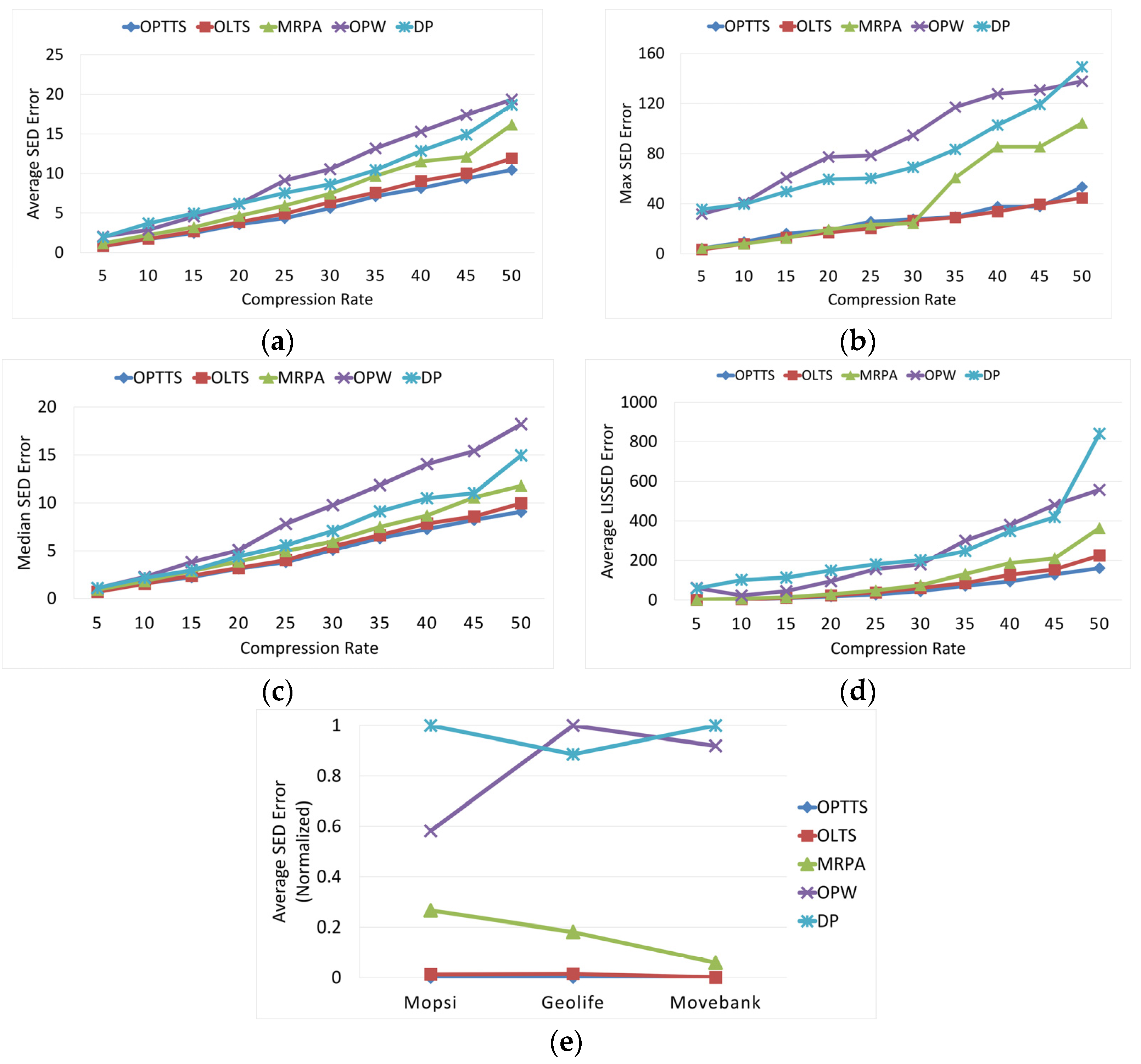
Average SED. Generally, smaller average SED error indicates better compression results. As shown in Figure 14a, the average SED error increases as the compression rate grows. OPTTS has the smallest error at each compression rate, followed by OLTS. The average SED error of OLTS is reduced by 40.8%, while the SED error of OPTTS is reduced by 45.6%.
Max SED. Max SED error is used to evaluate the stability of TS algorithms. The gentler the upward trend of the curve, the more stable of the algorithm. Figure 14b shows that OPTTS and OLTS have stable performance under different compression rates. The maximum value is 3~4 times of the average value. However, OPW, D-P, and MRPA have large fluctuation as the compression rates increase. The maximum values have a sudden surge to 6~8 times of the average values.
Median SED. Abnormal large value of SED may increase the average value, so it is insufficient to measure the performance only by average SED error. Median SED error is chosen as the auxiliary condition of average SED. As shown in Figure 14c, the situation of the median values are similar to the average values. OPTTS still has the smallest error, followed by OLTS.
Average ISSED. Average ISSED measures the overall approximation error of the compressed trajectory, which is also the optimization goal. Figure 14d shows that OPTTS has the lowest average LISSED error, followed by OLTS. OPTTS reduces the LISSED error by 82.2% compared to traditional algorithms, while OLTS reduces the error by 77.1%.
Average SEDs on different datasets. Average 
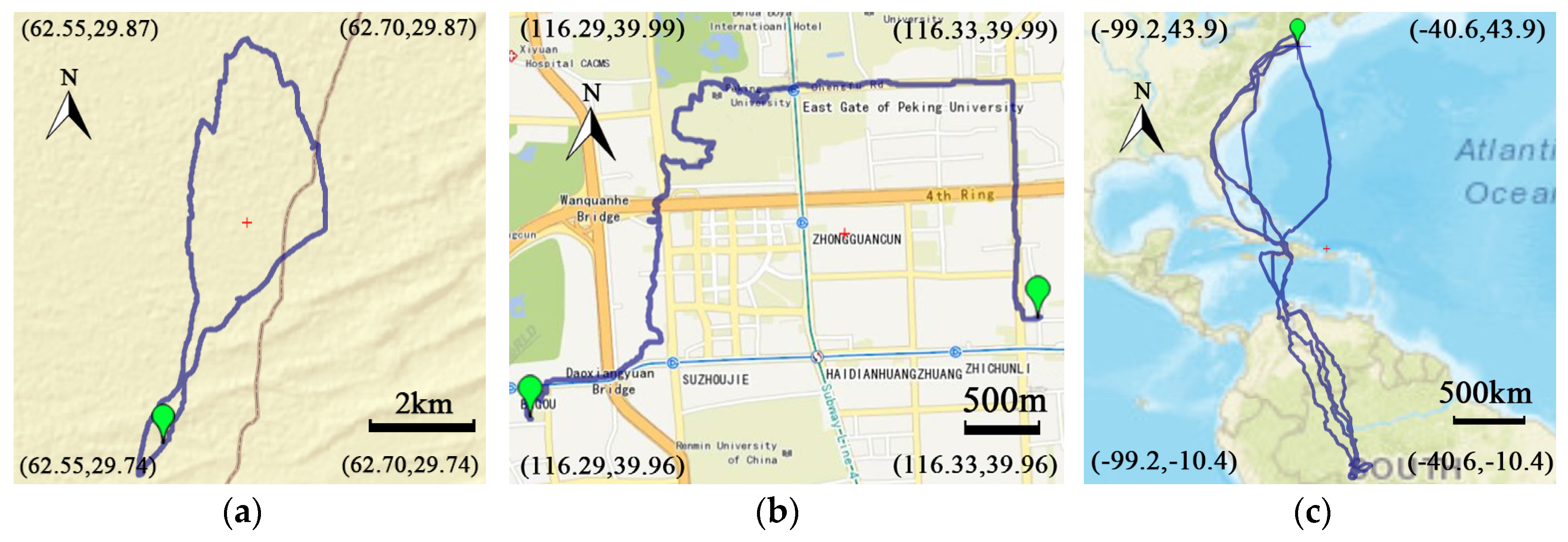
SED error is used to evaluate the robustness of the algorithms under different datasets. Three representative trajectories are selected respectively from Geolife, Mopsi, and Movebank datasets. Average SED error is calculated with fixed compression ratio γ = 10 . For better comparison, max-min normalization is utilized to unify different datasets to the same reference system. Figure 14e shows that OPTTS and OLTS perform relatively stable on all datasets, while OPW, D-P, and MRPA show a large fluctuation.
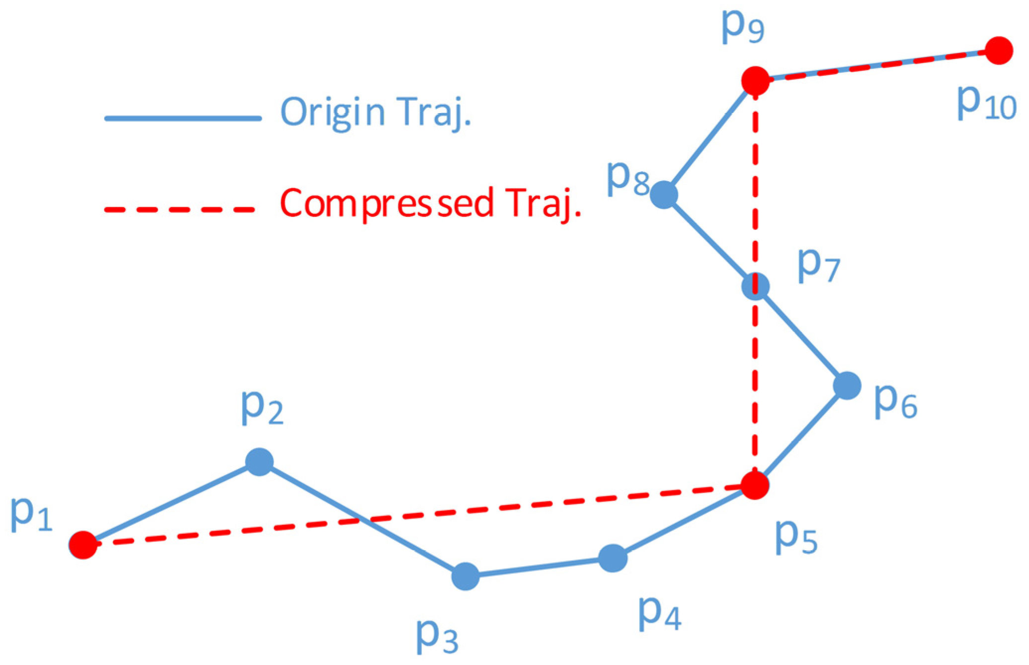
Visualization of Compression Result. The approximation error represents the deviation between the compressed and the original trajectory. It can be seen intuitively from the graphical representation of trajectories how large the difference is. Figure 15 shows the visualization of the compressed and the original trajectories by different algorithms. The same trajectory in the evaluation of error metrics is selected and the compression ratio is set to 100. In Figure 15a–d, the blue line always represents the original trajectory and the red one represents the result of OPTTS. The green lines respectively show the results of OLTS, MRPA, OPW, and D-P. It can be seen from Figure 15d that the compressed trajectory of D-P has the largest deviation, and the result of OPTTS is the most accurate representation of the original trajectory.
Experiment settings. Time cost is measured through two aspects, namely the number of points and compression rate. First, a trajectory from Geolife is selected and compression is executed every 5000 points from 5000 to 40,000 with a fixed rate γ = 10 . When exploring the relationship with the compression rate, a trajectory from Mopsi is chosen and simplification is made at 10 different compression rates with a fixed number of points. All algorithms were implemented in C++ and run on a Windows (64 bit) platform with a 2.50 GHz i7 CPU and 8 GB RAM.
Effect of number of points. As illustrated in Figure 16a, time costs of all algorithms show an increasing trend with the growth of points. OLTS is 32.2% faster than the traditional online algorithm OPW, even 40.3% faster than offline algorithm MRPA. While OPTTS is slower compared to other algorithms.
Effect of compression rates. As shown in Figure 16b, time costs of D-P, OPW, and OPTTS do not change with compression ratio, while MRPA and OLTS show an upward trend. When the compression ratio is less than 20, OLTS runs ahead of the D-P, OPW, and OPTTS. OLTS is faster than MRPA when the compression ratio is higher than 20.

5.3. Evaluation Based on Delay/Gap Analysis

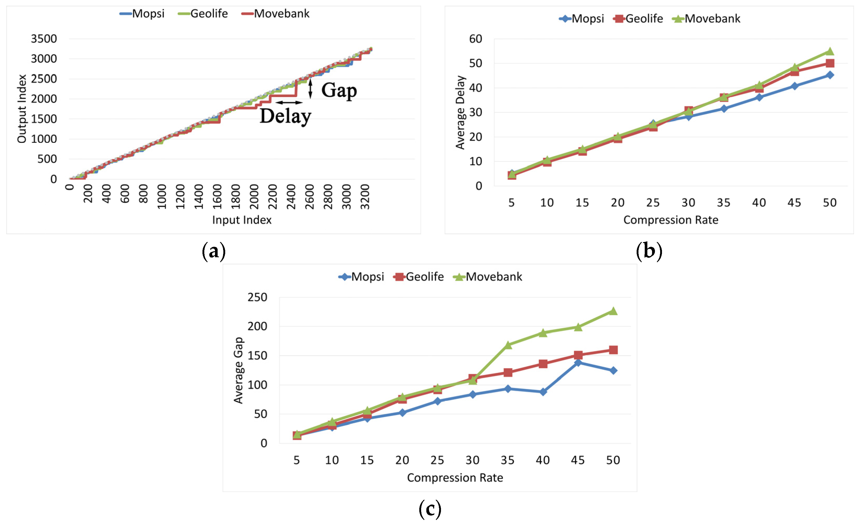
Visualization of delay and gap. Delay and gap are important features of OLTS. Three trajectories from Mopsi, Geolife, and Movebank with 3273 points are simplified on a fixed compression rate γ = 10 . The relationship between input index and output index is shown in Figure 17a. The Movebank dataset (red line) has the largest delay and gap. When the 2181st point is imported, the OLTS outputs the 2078th point. From the 2182nd to the 2457th point, there is no output of the algorithm. Until the input of the 2458th point, the 2160th point is output. Therefore, Delay = 2458 − 2181 and Gap = 2458 − 2160.
Average Delay. The relationship between delay and compression rate is shown in Figure 17b. The average delay is approximately equal to the compression rate in all datasets. Therefore, OLTS can guarantee a stable delay in various datasets.
Average Gap. The association between compression rate and average gap is shown in Figure 17c. Generally, OLTS’s gap becomes larger as the compression rate increases. The average gap of the Movebank dataset is the largest, followed by Geolife and Mopsi.

5.4. Discussion

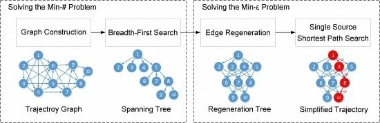
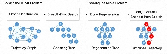
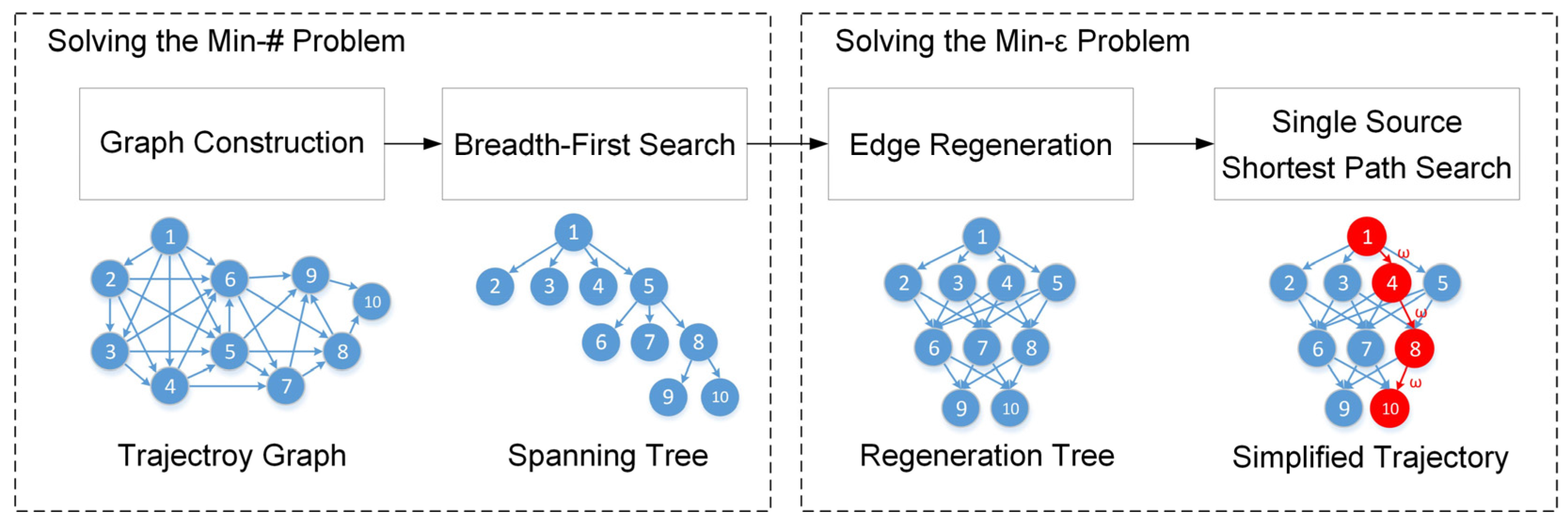
Effectiveness analysis. First, OPTTS has achieved the smallest result over all error metrics. OPTTS utilizes breadth-first spanning-regeneration tree and shortest path search to solve both min-# and min-ε problem and thus achieves the optimal solution. The approximation error of OLTS is slightly higher than OPTTS. Since OLTS extends the basic framework of OPTTS and utilizes a stopping criterion to speed up the construction of spanning tree, which leads to a near optimal result. However, D-P, OPW, and MRPA uses greedy strategy to improve efficiency, but the compression error is large. As is shown in Figure 15d, the green line representing the result of D-P has large deviation from the original trajectory. The performance of D-P may be unacceptable to some applications where the trajectory should be compressed as accurate as possible. For example, in some navigation applications, if the user’s trajectories compressed by D-P have a large approximation error, it may lead to deviation from the road map which is misleading. Secondly, OPTTS and OLTS have stable max SED errors since they use global optimal methods. However, D-P, OPW, and MRPA have abnormally large max SED at some parts of trajectory, due to the inappropriate selection of local optimization conditions. Finally, OPTTS and OLTS can achieve stable performance in all datasets. The influence of different features of the three datasets is reduced by the selection of an optimal method.
Time complexity analysis. Time complexity from theoretical derivation is summarized in Table 5. In the efficiency evaluation, D-P is the fastest among five algorithms, followed by OLTS and MRPA. D-P is heuristic-based and does not suffer from high complexity, while OPTTS utilizes optimization method during the construction of a breadth-first spanning regeneration tree, which is time consuming. However, the time cost of OPTTS is still acceptable to most offline applications, where the time cost is not considered as important as the performance of the compression. As is shown in Figure 15a, the time cost of OPTTS to a 1200 point trajectory is around 100 ms. It can be calculated that the total time cost for compressing all 14,638 trajectories in Geolife is about 24 min, which is tolerable. Thus, the improvement of compression effectiveness of OPTTS overwhelms the loss of computing efficiency. Furthermore, the time complexity of OLTS and MRPA is positively correlated with N/M, so the time cost rises as the increasing of compression rate. While OPTTS, OPW and D-P are only related to the number of points.
Delay and gap analysis. The proposed OLTS have uncertain delay and gap, introduced by the incremental construction of the breadth-first spanning tree and real-time output. The gap is correlated with the distance between V d and V k , and delay represents the number of nodes in each layer of the spanning tree, that is γ = N / M . First, local delay and gap may be influenced by the moving status of the object. As illustrated in Figure 17a, delay and gap have abnormally large values at some parts of the trajectory. This is because that the osprey may maintain a direct flight status for a long time. Secondly, average delay is approximately equal to compression rate. Because delay in OLTS represents the number of nodes in each layer of the spanning tree, which is equal to the compression rate. Finally, as illustrated in Figure 17c, the gap is 3~5 times of the compression rate, because the gap is related to the distance between V d and V k , which is bounded by O ( l o g N / M ) . Therefore, the gap should be in proportion to l o g γ in theory.

6. Conclusions

In order to solve the problem that heuristic-based algorithms may cause high approximation error, this paper presents an Optimal Trajectory Simplification Algorithm based on Graph Model (OPTTS). First, the optimal solution is defined as the compression schema with the minimum number of points as well as the minimum ISSED error. Then, a three-step algorithm is proposed to solve the optimal solution. By transferring trajectory into a graph model, breadth-first search is used to solve the min-# problem, followed by the single source shortest path search to solve the min-ε problem. Experimental study has illustrated that OPTTS lessens the approximation error by 82% compared to traditional methods. OPTTS works in batch mode and has a time complexity of O ( N 2 ) .
To extend OPTTS to online application, a new Online Trajectory Simplification Algorithm based on Directed Acyclic Graph (OLTS) is proposed, which follows the structure of OPTTS. Dealing with trajectory stream, OLTS dynamically constructs the breadth-first spanning tree with the stopping criterion to terminate the construction of each layer. Then the approximation error of the current layer is minimized, followed by the real-time output. OLTS achieves a near optimal solution that reduces the approximation error by 77%. Meanwhile, OLTS is 32% faster than the classic online algorithm. Both OPTTS and OLTS have stable effectiveness and time cost on different datasets.
There are several potential extensions of this paper. First, the stay points in trajectory are of great significance in mining point-of-interest and activity pattern recognition. [23,24]. However, the traditional TS algorithms reduce all stay points. The construction of a breadth-first tree in OPTTS and OLTS will be improved to reserve the stay point. Furthermore, multi-resolution display of trajectory is needed in many navigation applications. A huge amount of trajectory data in coarse resolution may cause the application to stall and crash [25,26]. Existing multi-resolution TS algorithms often work in batch mode. A key goal of our future work is to explore a new online multi-resolution TS method.

Acknowledgments

This paper is supported by the National Natural Science Foundation of China (No.41501485).

Author Contributions

Fan Wu and Kun Fu conceived and designed the experiments; Fan Wu and Zhibin Xiao performed the experiments; Fan Wu and Yang Wang analyzed the data; Fan Wu wrote the paper.

Conflicts of Interest

The authors declare no conflict of interest.

References

  1. Zheng, Y.; Zhou, X. Computing with Spatial Trajectories; Springer: New York, NY, USA, 2011. [Google Scholar]
  2. Meratnia, N.; de By, R.A. Spatiotemporal compression techniques for moving point objects. In Proceedings of the 9th International Conference on Extending Database Technology, Heraklion, Greece, 14–18 March 2004; pp. 765–782.
  3. Melkman, A.; O’Rourke, J. On polygonal chain approximation. In Computational Morphology; Elsevier Science: Amsterdam, The Netherlands, 1988; pp. 87–95. [Google Scholar]
  4. Salotti, M. Optimal polygonal approximation of digitized curves using the sum of square deviations criterion. Pattern Recognit. 2002, 35, 435–443. [Google Scholar] [CrossRef]
  5. Imai, H.; Iri, M. Polygonal approximations of a curve-formulations and algorithms. In Computational Morphology; Elsevier Science: Amsterdam, The Netherlands, 1988; pp. 71–86. [Google Scholar]
  6. Chen, M.; Xu, M.; Fränti, P. A fast multiresolution polygonal approximation algorithm for GPS trajectory simplification. IEEE Trans. Image Process. 2012, 21, 2770–2785. [Google Scholar] [CrossRef] [PubMed]
  7. Douglas, D.H.; Peucker, T.K. Algorithms for the reduction of the number of points required to represent a digitized line or its caricature. Cartogr. Int. J. Geogr. Inf. Geovis. 1973, 10, 112–122. [Google Scholar] [CrossRef]
  8. Pikaz, A. An algorithm for polygonal approximation based on iterative point elimination. Pattern Recognit. Lett. 1995, 16, 557–563. [Google Scholar] [CrossRef]
  9. Agarwal, P.K.; Varadarajan, K.R. Efficient algorithms for approximating polygonal chains. Discret. Comput. Geom. 2000, 23, 273–291. [Google Scholar] [CrossRef]
  10. Daescu, O.; Mi, N. Polygonal chain approximation: A query based approach. Comput. Geom. Theory Appl. 2005, 30, 41–58. [Google Scholar] [CrossRef]
  11. Kolesnikov, A.; Fränti, P. Reduced-search dynamic programming for approximation of polygonal curves. Pattern Recognit. Lett. 2003, 24, 2243–2254. [Google Scholar] [CrossRef]
  12. Potamias, M.; Patroumpas, K.; Sellis, T. In sampling trajectory streams with spatiotemporal criteria. In Proceedings of the 18th International Conference on Scientific and Statistical Database Management, Vienna, Austria, 3–5 July 2006; pp. 275–284.
  13. Vitter, J.S. Random sampling with a reservoir. ACM Trans. Math. Softw. 1985, 11, 37–57. [Google Scholar] [CrossRef]
  14. Keogh, E.; Chu, S.; Pazzani, M. An online algorithm for segmenting time series. In Proceedings of the 2001 IEEE International Conference on Data Mining, San Jose, CA, USA, 29 November–2 December 2001; pp. 289–296.
  15. Muckell, J.; Olsen, P.W.; Hwang, J.H.; Lawson, C.T.; Ravi, S.S. Compression of trajectory data: A comprehensive evaluation and new approach. Geoinformatica 2014, 18, 435–460. [Google Scholar] [CrossRef]
  16. Lawler, E.L. Combinatorial optimization: Networks and matroids. Bull. Am. Math. Soc. 2001, 84, 461–463. [Google Scholar]
  17. Dijkstra, E.W. A note on two problems in connexion with graphs. Numer. Math. 1959, 1, 269–271. [Google Scholar] [CrossRef]
  18. Chen, D.Z.; Daescu, O. Space-efficient algorithms for approximation polygonal curves in two-dimentional space. Int. J. Comput. Geom. Appl. 2003, 13, 135–142. [Google Scholar] [CrossRef]
  19. Kolesnikov, A.; Fränti, P. A fast near-optimal min-# polygonal approximation of digitized curves. In Proceedings of the IASTED International Conference on Automation, Control and Information Technology-ACIT’02, Novosibirsk, Russia, 10–13 June 2002; pp. 418–422.
  20. Mopsi Project. Available online: http://cs.joensuu.fi/mopsi/ (accessed on 3 October 2016).
  21. Zheng, Y.; Xie, X.; Ma, W.Y. Geolife: A collaborative social networking service among user, location and trajectory. IEEE Data Eng. Bull. 2010, 33, 32–39. [Google Scholar]
  22. Movebank. Available online: http://www.movebank.org (accessed on 3 October 2016).
  23. Xiang, L.; Gao, M.; Wu, T. Extracting stops from noisy trajectories: A sequence oriented clustering approach. ISPRS Int. J. Geo-Inf. 2016, 5, 29. [Google Scholar] [CrossRef]
  24. Fu, Z.; Tian, Z.; Xu, Y.; Qiao, C. A two-step clustering approach to extract locations from individual GPS trajectory data. ISPRS Int. J. Geo-Inf. 2016, 5, 166. [Google Scholar] [CrossRef]
  25. Kolesnikov, A.; Franti, P.; Wu, X. Multiresolution polygonal approximation of digital curves. In Proceedings of the 17th International Conference on Pattern Recognition, ICPR 2004, Cambridge, UK, 23–26 August 2004; Volume 2, pp. 855–858.
  26. Marteau, P.F.; Nier, G. Speeding up simplification of polygonal curves using nested approximations. Pattern Anal. Appl. 2009, 12, 367–375. [Google Scholar] [CrossRef]
Figure 1. Illustration of trajectory simplification. The original trajectory consists of ten points and the simplified trajectory contains four points, namely { p 1 , p 5 , p 9 , p 10 } .
Ijgi 06 00019 g001
Figure 2. (a) Enumeration of all compression schemas of a trajectory that contains 16 points. Each point in the graph represents a simplified track with M points and Y-axis shows the ISSED error. (b) Min-# problem is to find the minimum value of M below the error threshold, which is four below the horizontal red line. Min-ε problem is to find the minimum ISSED under the M-threshold, which is the lowest point along the vertical red line.
Ijgi 06 00019 g002
Figure 3. Flow chart of the OPTTS.
Ijgi 06 00019 g003
Figure 4. (a) The process of the Edge Test. (b) The trajectory graph.
Ijgi 06 00019 g004
Figure 5. (a) The process of the breadth-first search. (b) The breadth-first spanning tree.
Ijgi 06 00019 g005
Figure 6. (a) The process of the breadth-first search. (b) The breadth-first spanning tree.
Ijgi 06 00019 g006
Figure 7. Regeneration Tree.
Ijgi 06 00019 g007
Figure 8. Flow chart of the OLTS.
Ijgi 06 00019 g008
Figure 9. Dynamic construction of the spanning tree.
Ijgi 06 00019 g009
Figure 10. Running example of stopping criterion.
Ijgi 06 00019 g010
Figure 11. Running example of the output process.
Ijgi 06 00019 g011
Figure 12. The m generation of ancestors of V k .
Ijgi 06 00019 g012
Figure 13. (a) Mopsi: A jogging track in a park in Helsinki, Finland. (b) Geolife: A track of a student traveling from home to school in Beijing, China. (c) Movebank: A three-year track (January 2006~December 2008) of an osprey migrating from the United States to Brazil.
Ijgi 06 00019 g013
Figure 14. (a) Average SED error. (b) Max SED error. (c) Median SED error. (d) Average ISSED error. (e) Average SED errors on different datasets.
Ijgi 06 00019 g014
Figure 15. Visualization of compressed trajectories by different algorithms. (a) OPTTS vs. OLTS. (b) OPTTS vs. MRPA. (c) OPTTS vs. OPW. (d) OPTTS vs. D-P.5.3. Evaluation Based on Time Cost.
Ijgi 06 00019 g015
Figure 16. (a) Time cost of different number of points. (b) Time cost of different compression rates.
Ijgi 06 00019 g016
Figure 17. (a) Visualization of delay and gap. (b) Average delay. (c) Average gap.
Ijgi 06 00019 g017
Table 1. Classification of TS algorithms.
HeuristicOptimalHybrid
CurveOfflineSimple SimplifyGraph-BasedRSDP
Douglas–PeuckerIterative Map
MergingPriority Quere
TrajectoryOfflineThresholdOPTTS 1MRPA
Time Ratio
OnlineUniform Sample OLTS 1
Open Window
ST-Trace
Squish-E
1 OPTTS and OLTS are proposed in this paper.
Table 2. Statistics of three example trajectories.
DatasetPointsAvgRate (sec)AvgDis (m)StdDis (m2)AvgSpd (m/s)StdSpd (m2/s2)
Mopsi37472.2106.34.52.1
Geolife32732.616.55.77.95.9
Movebank12,3802 h380013,00012.3
Table 3. Characteristics of compared algorithms.
SceneProposed AlgorithmModeCompared AlgorithmMode
OfflineOPTTSOptimalD-PHeuristics
MRPAHybrid
OnlineOLTSHybridOPW Heuristics
Table 4. Abbreviation and calculation formula of different error metrics.
Error MetricAbbr.Calculation Formula
Average SED Error S E D a v g S E D a v g = k = 1 N S E D ( p k , p k ) / N
Max SED Error S E D m a x S E D m a x = max 1 k N { S E D ( p k , p k ) }
Median SED Error S E D m e d S E D m e d = median 1 k N { S E D ( p k , p k ) }
Average ISSED Error I S S E D a v g I S S E D a v g = p k i T L I S S E D ( T k i k i + 1 ) / N
Table 5. Time complexity of five algorithms.
AlgorithmOPTTSOLTSMRPAOPWD-P
Time complexity O ( N 2 ) O ( N 2 / M ) O ( N 2 / M ) O ( N 2 ) O ( N l o g N )

