sgdm: An R Package for Performing Sparse Generalized Dissimilarity Modelling with Tools for gdm

Abstract

Global biodiversity change creates a need for standardized monitoring methods. Modelling and mapping spatial patterns of community composition using high-dimensional remotely sensed data requires adapted methods adequate to such datasets. Sparse generalized dissimilarity modelling is designed to deal with high dimensional datasets, such as time series or hyperspectral remote sensing data. In this manuscript we present sgdm, an R package for performing sparse generalized dissimilarity modelling (SGDM). The package includes some general tools that add functionality to both generalized dissimilarity modelling and sparse generalized dissimilarity modelling. It also includes an exemplary dataset that allows for the application of SGDM for mapping the spatial patterns of tree communities in a region of natural vegetation in the Brazilian Cerrado.

1. Introduction

Global biodiversity change may lead to declines and changes in ecosystem functioning and provisioning of services [1], which presents the need for standardized methods capable of extracting useful information from in situ biological observations for the use of global biodiversity monitoring [2,3]. In particular, it is highly relevant to characterize species community composition and turnover, as they directly relate to ecosystem functioning [4,5]. Modelling biodiversity at the community level has several advantages in relation to modelling individual species, as it allows for the incorporation of rare species through the detection of shared patterns of environmental responses across species, while directly predicting community composition and turnover [6,7]. Furthermore, it avoids the problems of stacking individual-species models with varying explanatory powers, which generally leads to biased inference [8]. The two main approaches used for modelling species communities are those based on data ordination, such as canonical correlation analysis [5], or through dissimilarity measures [9,10]. Generalized dissimilarity modelling (GDM) is a well-established dissimilarity-based statistical technique for analysing and predicting biological variation as a function of environment [10]. It specifically relates dissimilarity in the composition of a biological community (e.g., differences in species or traits) between pairs of sites with the respective environmental difference as described by the predictors. This is done through a linear combination of I-spline (monotonical) basis functions, following the assumption that increasing separation of sites along an environmental gradient can only result in increasing compositional dissimilarity [10]. The dissimilarity predictions generated by GDM can be used to visualize the spatial pattern in community compositional change through a subsequent non-linear ordination. GDM is thus a useful tool for assessing biodiversity change across large areas, although its potential for widespread use depends on the availability of standardized high quality environmental data.

Remotely sensed data are particularly suitable for the global and systematic description of ecological processes and the environment [11,12]. Remote sensing data products, such as long time series of optical satellite data, or spaceborne hyperspectral imagery, allow the description of the Earth’s surface with an unprecedented quality and detail [13,14]. This provides ecologists with great opportunities for their usage in biodiversity assessments [15,16]. The choice of suitable remote sensing variables for modelling biodiversity is, however, an area of ongoing research [17]. While the use of continuous remotely sensed information, such as spectral indices or time series data, has been shown to be useful for characterising species distributions [18,19], the high-dimensional (and potentially multicollinear) nature of these data poses challenges for analysis [20], which typically results in loss of model performance and generalization.

Recently, a methodological enhancement was developed that allows for fitting high-dimensional data in GDM. This enhancement is called sparse generalized dissimilarity modelling (SGDM) [21] and is a two-stage approach that consists of initially reducing the environmental data (i.e., predictor variables) by means of a sparse canonical correlation analysis (SCCA) [22], and then fitting the resulting transformed environmental space with a GDM model. The SCCA is a form of penalized canonical correlation analysis, thus transforming both biological and environmental data matrices in order to maximise the correlation between both. The penalization in SCCA is done via the L1 (lasso) penalty function, which is designed to deal with high-dimensional and multi-collinear datasets [23,24]. SCCA reduces high-dimensional data while simultaneously allowing for the extraction of environmental information related to the community data variability. For running a SCCA, it is necessary to define the penalization parameter to be applied to each of the environmental and community data matrices. In SGDM, the parameterization is done in a heuristic grid search manner, in order to minimize the residuals (in the form of the cross-validated root mean square error; RMSE) in the predicted dissimilarities of a GDM model [21].

SGDM has proven useful for performing generalized dissimilarity modelling with high-dimensional remote sensing data [21]. While the GDM modelling approach is implemented in the gdm R package and available from the CRAN repository [25,26], there is yet no implementation of SGDM available to ecologists and environmental researchers. In times of increasing availability of remote sensing data, and the consequent increase in dimensionality, it is highly relevant that useful tools capable of dealing with these data are available to the global ecologist community. In the current paper, we aim to fill this gap and thus present sgdm, an R package for performing sparse generalized dissimilarity modelling, including some additional tools suitable for both SGDM and GDM.

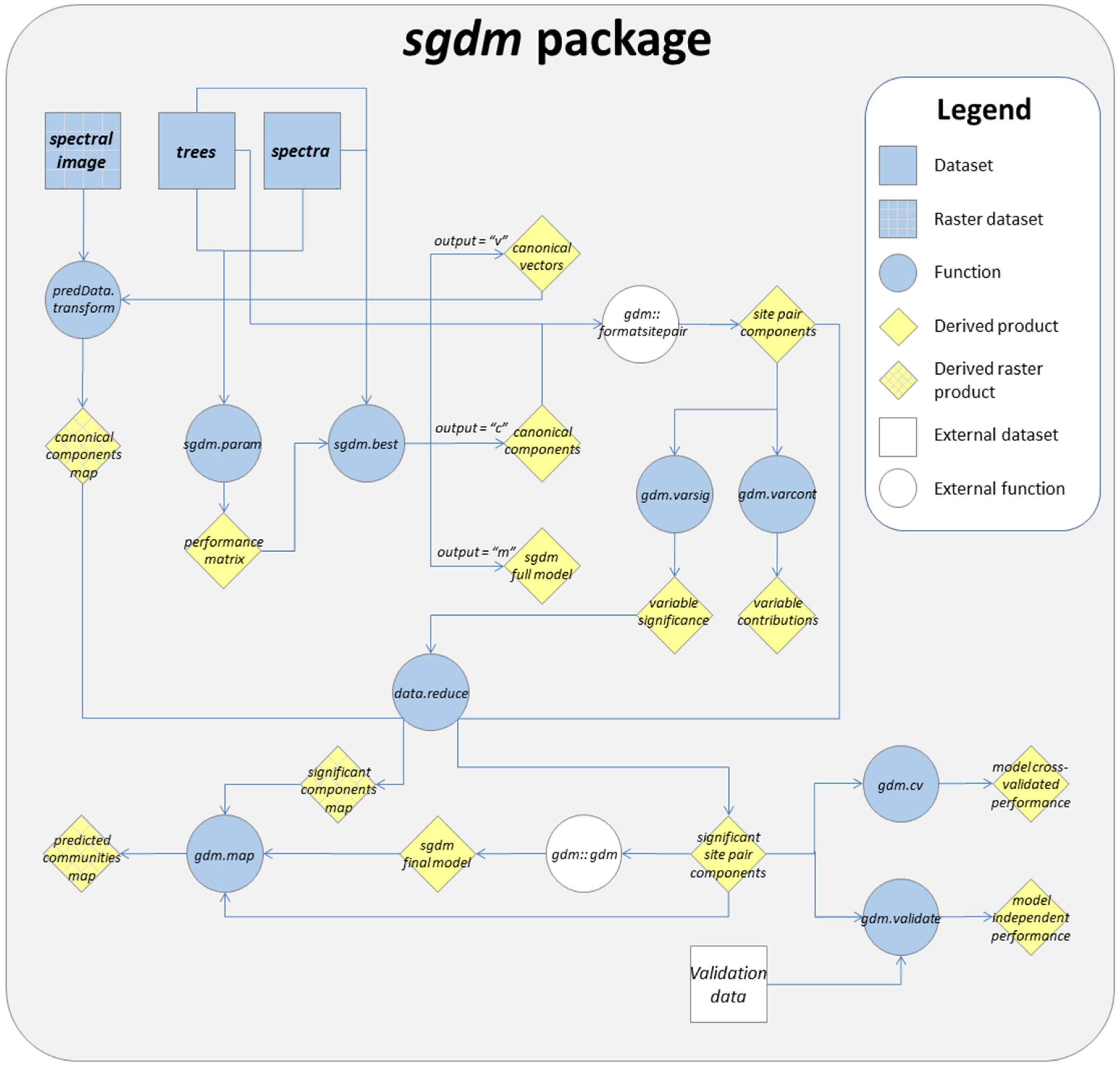
2. General sgdm Package Description

The sgdm package is available from GitHub (https://github.com/sparsegdm/sgdm_package), and depends on the installation of a few other R packages in order to run. Namely it requires the gdm package [25] for running the GDM model, the PMA package [27] for running the SCCA, and the vegan package [28] for several internal operations. The functions for spatially explicit mapping the model results further require the installation of the raster [29] and the yalmpute [30] packages. The sgdm package can be directly installed and loaded in R using the following commands:

• R> # Package installation from GitHub
• R> devtools::install_github("sparsegdm/sgdm_package")
• R> Loading package
• R> library(sgdm)

The package includes nine functions and three exemplary datasets. In Figure 1 we present all functions and datasets, as well as a possible workflow to derive a raster map of Cerrado tree communities based on the exemplary datasets.

The datasets provided with the package include one biological dataset and one predictor dataset (both as data frames), as well as one predictor map as raster object (Figure 2). The trees biological dataset is composed of 30 observations with abundance values for 48 different tree families in a region of natural vegetation in the Brazilian Cerrado. The spectra predictor dataset is composed of the same 30 observations, with reflectance values for 83 narrow spectral bands covering the visible, near-, and shortwave-infrared portions of the electromagnetic spectrum. The spectra have been extracted from spaceborne hyperspectral Hyperion imagery acquired on 27 June 2014, after pre-processing and band quality screening. Both datasets include an ID column and the latter also includes two geographical coordinate columns (X and Y). The spectral.image predictor map constitutes a subset (100 × 100 pixels) of the respective Hyperion image.

3. Running a SGDM Model in the sgdm Package

In order to run a SGDM model in the sgdm package it is necessary to parameterize the built-in SCCA, which includes defining the penalization values to be applied in the lasso-based canonical transformation for both the biological and environmental matrices. This is done via a heuristic grid search by testing combinations of parameter pairs using the sgdm.param function. In the grid search, all possible parameter pairs are tested in a five-fold cross-validation and optimized by minimizing the root mean square error (RMSE) between predicted and observed dissimilarities between sample pairs. The penalization values to be tested can range from 0 (strong penalization) to 1 (weak penalization). As described by Leitão et al. [21], high levels of penalization (low penalization values) should be avoided in order to assure a strong association between the transformed predictor and biological data. Following this recommendation, the default penalization values (for both data matrices) in the sgdm package range from 0.6 to 1 in steps of 0.1, although these values can be manually configured to better match the user needs (for example, datasets with higher dimension might require higher levels of penalization). The sgdm.param function also requires the definition of the number of components to be extracted in the SCCA, the distance metric to be used in the GDM models, and the optional use of geographical distance as a variable in the GDM model. As suggested in the method description [21], the maximum possible number of components (i.e., the number of samples) should be initially used to be later reduced to the statistical significant ones. Although this option is available here, the use of geographical distance as a variable remains untested with SGDM. Note that the current implementation of this function only allows for biological abundance data, described as format 1 in the gdm package [25]. The SGDM model parameterization function is called by:

• R> # Parameterize SGDM
• R> sgdm.gs <− sgdm.param(predData = spectra, bioData = trees, k = 30)

The sgdm.param function delivers a performance matrix with the RMSE values for each parameter pair tested in the SGDM model (Figure 3). In this case, the best model corresponds to the use of a penalisation value of 0.7 on both the environmental and biological matrices, resulting in a RMSE value of 0.114.

In order to run the best SGDM model (following the parameterization step), this matrix can be fed into the sgdm.best function:

• R> # Retrieving and building the best SGDM model
• R> sgdm.model <− sgdm.best(perf.matrix = sgdm.gs, predData = spectra, bioData = trees, output = ”m”, k = 30)

The previous step originated a GDM model with 30 predictor variables, i.e., the 30 canonical components generated in the SCCA (with penalisation values of 0.7 for both matrices), and explained 73.36% of the deviance (corresponding to the model’s fit performance). By inspecting the GDM model (with the summary.gdm function of the gdm package), it is possible to verify, however, that not every predictor variable was effectively used in the model. Indeed, in the given example, only 12 variables had at least one non-zero coefficient.

Alternatively, the sgdm.best function also allows the user to retrieve the resulting sparse canonical components or the respective canonical vectors by respectively setting the output argument to “c” or “v”. The code below shows the code necessary to retrieve the resulting sparse canonical components and vectors, using the exemplary data:

• R> # Retrieving the sparse canonical components corresponding to the best GDM model
• R> sgdm.sccbest <− sgdm.best(perf.matrix = sgdm.gs, predData = spectra, bioData = trees, output = ”c”, k = 30)
• R> # Retrieving the sparse canonical vectors corresponding to the best GDM model
• R> sgdm.vbest <− sgdm.best(perf.matrix = sgdm.gs, predData = spectra, bioData = trees, output = ”v”, k = 30)

The selected canonical transformation can also be applied to the prediction map to allow for the spatial prediction of the SGDM model. This can be done with the predData.transform function, as shown below.

• R> # Applying SCCA transformation onto the prediction map
• R> component.image <− predData.transform(predData = spectral.image, v = sgdm.vbest)

The following steps of the SGDM approach relate to the model simplification following a significance test [21]. The functions provided to perform this are not specific of SGDM, but are rather useful for GDM in general.

4. Additional Tools Useful for GDM and SGDM

In addition to the above described specific functions, the sgdm package also provides some general functions that add functionality to both SGDM and GDM. The variable drop contributions of a GDM model can be calculated through the function gdm.varcont, which excludes each single variable at once and calculates the respective loss in model deviance explained. The significance of the variable contributions can be checked with the gdm.varsig function, as these are tested against randomness via permutations of the biological data matrix [10]. The significance level to which the variable contributions are tested is set to p < 0.05 per default, though it can be manually defined. This function delivers a vector with the same length as the number of variables, with logical values indicating whether the variables’ contributions are significant or not—all variables with no contribution are automatically assigned as non-significant. Following the significance test, the models can be simplified by excluding the non-significant variables using the data.reduce function. The code below exemplifies the variable contributions and significance checks, followed by the respective exclusion of non-important variables and retrieval of the final (reduced) model, using the exemplary data.

• R> # Combining pair site data for GDM model variable contribution check
• R> spData.sccbest <− gdm:: formatsitepair(bioData = trees, bioFormat = 1, dist = "bray", abundance = TRUE, siteColumn = "Plot_ID", XColumn = "X", YColumn = "Y", predData = sgdm.sccbest)
• R> # Checking SGDM variable drop contribution
• R> gdm.varcont(spData = spData.sccbest)
• R> # Checking significance of variable contributions
• R> sigtest.sgdm <− gdm.varsig(predData = sgdm.sccbest, bioData = trees)
• R> # Excluding non-significant variables
• R> sgdm.sccbest.red <− data.reduce(data = sgdm.sccbest, datatype = "pred", sigtest = sigtest.sgdm)
• R> # Combining pair site data for input in GDM
• R> spData.sccbest.red <− gdm:: formatsitepair(bioData = trees, bioFormat = 1, dist = "bray", abundance = TRUE, siteColumn = "Plot_ID", XColumn = "X", YColumn = "Y", predData = sgdm.sccbest.red)
• R> # Final SGDM model
• R> sgdm.model.red <− gdm:: gdm(data = spData.sccbest.red)

In this case, the model reduction resulted in a final GDM model with six predictor variables which explained 70.09% of the deviance within the data. The fitted model and corresponding I-splines can be plotted using the plot.gdm function of the gdm package (Figure 4).

For further inspection of the final model results, the predicted dissimilarities can be plotted against the observed dissimilarities between all site pairs (Figure 5). This gives good insight into the distribution of the dissimilarity values, as well as of the model predictions.

The package also includes two functionalities for GDM model validation. Namely, the gdm.cv function that performs n-fold model cross-validation, and the gdm.validate function which performs model validation using an independent dataset. This function can calculate both RMSE and r-square (calculated based on the squared Pearson correlation coefficient). As an example, the GDM cross-validation can be performed using:

• R> # 10-fold cross-validation of the final SGDM model
• R> gdm.cv(spData = spData.sccabest.red, nfolds = 10, performance = "r2")

In this example, the final (reduced) model presented a cross-validated r-square of 64.34%. On the other hand, by comparing it with a GDM model built with the (significant) original spectral bands (4 out of 83; without prior SCCA transformation), it can be observed that the latter resulted in a weaker cross-validated performance (r-square of 53.38%).

The main community composition patterns can be mapped along the main axes of variation between the predicted dissimilarities between all pairs of sites through applying a non-metric multidimensional scaling (NMDS) transformation [10]. This transformation is implemented in the gdm.map function of the sgdm package, which uses the monoMDS function implemented in the vegan package. It requires the definition of the number of NMDS axes to be extracted, which can be done manually or automatically based on NMDS stress values [31]:

• R> # Mapping community composition
• R> map.sitepairs <− gdm.map(spData = spData.sccabest.red, model = sgdm.model.red)

In this example, the number of NMDS components to be derived was set automatically (using the default stress value threshold of 0.1), which resulted in eight components. These eight components summarised most of the variance in the tree community structure present in the study area.

The model predictions can be extrapolated to the whole study area, as described by the predictor map. As it would be unfeasible to run a NMDS on the dissimilarities between all possible pairs of image pixels [10], it is possible to assign the pixels to the NMDS axes from the sample pairs through a knn-imputation [32]. This requires the reduction of the canonical component map (obtained from the predData.transform function) into the significant components, using the data.reduce function. Finally, when including a prediction image (e.g., the map of the significant components) as an argument in the gdm.map function, this will assign the image pixels along the NMDS axes, as calculated for the sample pairs. This procedure results in the spatially explicit mapping of the community composition patterns throughout the study area. A mapping example is given below:

• R> # Reducing canonical component map to significant components
• R> component.image.red <− data.reduce(data = component.image, datatype = "pred", igtest = sigtest.sgdm)
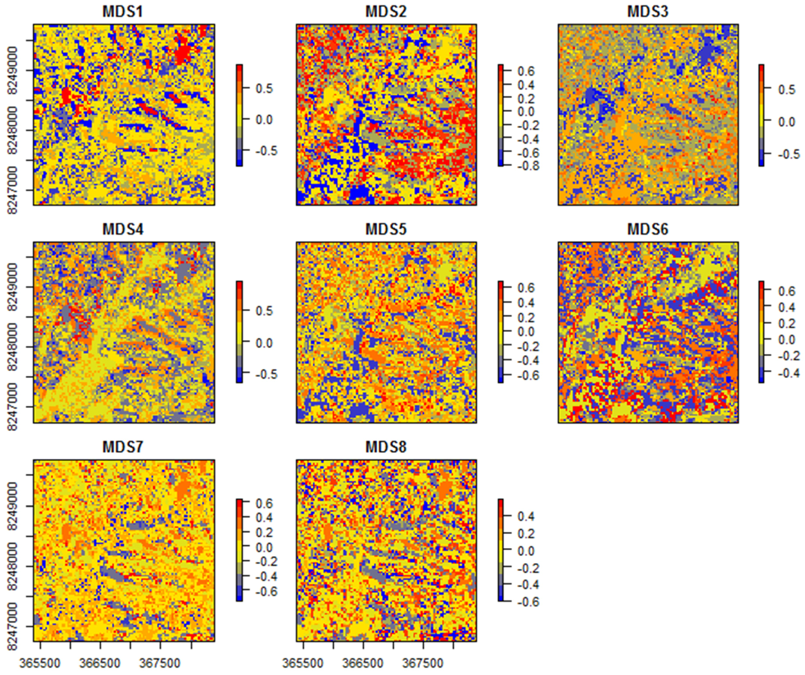
• R> # Mapping community composition in space
• R> map.image <− gdm.map(spData = spData.sccabest.red, predMap = component.image.red, model = sgdm.model.red, k = 8)

In this last example, the main patterns of community transition are plotted, according to the eight NMDS ordinations of the SGDM model predictions (Figure 6).

By inspecting the resulting maps it can be observed that different aspects of the community transition are depicted by different NMDS axes. For example, the first axis mostly represents species turnover within typical savanna areas (blue to red), whereas the second axis rather represents turnover between forested (blue) and savanna (red) regions. The third axis, however, mostly depicts the species turnover between sparser (blue) and denser (red) savanna formations—this inference can be done for all resulting axes. Cross-checking the resulting NDMS axes with the corresponding species community (for the samples) provides further insights for a senseful inference of the modelled spatial patterns. In this case study, the high tree taxonomic diversity of the Cerrado is well depicted in the rather large number of resulting NMDS axes. The high heterogeneity of this system results in the “salt-and-pepper” pattern visible on most NMDS axes.

5. Discussion

The sgdm package allows for the use of high-dimensional data, such as hyperspectral or time series remote sensing data, in a GDM modelling framework for mapping the spatial patterns of species communities across large areas. Indeed, in the illustrated case study, we used a hyperspectral image from the Hyperion satellite sensor to successfully map tree community transitions in the Brazilian Cerrado. The resulting model included six significant variables (canonical components), which were condensed from the 83 original spectral bands and thereby led to a considerable improvement in the respective predictive (cross-validated) model performance.

Unlike the GDM model itself (which is deterministic), the SGDM approach is a probabilistic approach, as its parameterization depends on a heuristic grid search based on a cross-validation procedure [21]. This means that several runs of the SGDM model on the same data may result in slightly different model parameters, with resulting different model performances and predicted patterns, which may bring some instability in the model parameterization. We found that, by setting the default parameters to moderate to weak penalization (from 0.6 to 1), as recommended in the method description [21], the resulting parameter selection was robust. This has, however, not been analysed in depth and requires further research. Furthermore, the best penalization parameter pair is fully data dependent and the candidate parameter pairs to be tested in the grid search might need to be adapted to the datasets used. Indeed, datasets with very high dimensionality might need higher levels of penalization (lower parameter values) than those with lower dimensionality.

Mapping spatial patterns of community composition using a spectral image over a geographically large region is not simple and straightforward. Ideally, the dissimilarities between all image pixel pairs would be predicted from the GDM or SGDM model, and then transformed using NMDS. However, for large regions (i.e., millions of pixels) these steps are unfeasible due to the computation resources needed [10,21]. In the current package implementation an alternative approach was suggested, where the image pixels are assigned to the NMDS axes through a nearest neighbour imputation approach [32]. This delivers a map of pixels with similar communities depicting the community turnover through space, with varying environmental conditions. An alternative approach, currently not implemented in the sgdm package, is to recur to a regression approach to assign the image pixels along the NMDS axes.

6. Conclusions

The package presented in this study is a running implementation of the SGDM methodological approach and is available online (on GitHub) under a Creative Commons license for generalized use. This release thus allows for the modelling and mapping of turnover in community structure over geographically large regions by facilitating the use of high-dimensional data from existing and forthcoming new generations of Earth observation satellites in a GDM framework.

References

1. Chapin, F.S., III; Zavaleta, E.S.; Eviner, V.T.; Naylor, R.L.; Vitousek, P.M.; Reynolds, H.L.; Hooper, D.U.; Lavorel, S.; Sala, O.E.; Hobbie, S.E.; et al. Consequences of changing biodiversity. Nature 2000, 405, 234–242. [Google Scholar] [CrossRef] [PubMed]
2. Pereira, H.M.; Navarro, L.M.; Martins, I.S. Global biodiversity change: the bad, the good, and the unknown. Annu. Rev. Environ. Resour. 2012, 37, 25–50. [Google Scholar] [CrossRef]
3. Ferrier, S. Extracting more value from biodiversity change observations through integrated modeling. BioScience 2011, 61, 96–97. [Google Scholar] [CrossRef]
4. Hooper, D.U.; Chapin, F.S.; Ewel, J.J.; Hector, A.; Inchausti, P.; Lavorel, S.; Lawton, J.H.; Lodge, D.M.; Loreau, M.; Naeem, S.; et al. Effects of biodiversity on ecosystem functioning: A consensus of current knowledge. Ecol. Monogr. 2005, 75, 3–35. [Google Scholar] [CrossRef] [Green Version]
5. Legendre, P.; Borcard, D.; Peres-Neto, P.R. Analyzing beta diversity: Partitioning the spatial variation of community composition data. Ecol. Monogr. 2005, 75, 435–450. [Google Scholar] [CrossRef]
6. Guisan, A.; Weiss, S.B.; Weiss, A.D. GLM versus CCA spatial modeling of plant species distribution. Plant Ecol. 1999, 143, 107–122. [Google Scholar] [CrossRef]
7. Ferrier, S.; Guisan, A. Spatial modelling of biodiversity at the community level. J. Appl. Ecol. 2006, 43, 393–404. [Google Scholar] [CrossRef]
8. Guisan, A.; Rahbek, C. SESAM—A new framework integrating macroecological and species distribution models for predicting spatio-temporal patterns of species assemblages. J. Biogeogr. 2011, 38, 1433–1444. [Google Scholar] [CrossRef]
9. De Caceres, M.; Legendre, P.; He, F. Dissimilarity measurements and the size structure of ecological communities. Methods Ecol. Evolut. 2013, 4, 1167–1177. [Google Scholar] [CrossRef]
10. Ferrier, S.; Manion, G.; Elith, J.; Richardson, K. Using generalized dissimilarity modelling to analyse and predict patterns of beta diversity in regional biodiversity assessment. Divers. Distrib. 2007, 13, 252–264. [Google Scholar] [CrossRef]
11. Kerr, J.T.; Ostrovsky, M. From space to species: Ecological applications for remote sensing. Trends Ecol. Evolut. 2003, 18, 299–305. [Google Scholar] [CrossRef]
12. Jetz, W.; Cavender-Bares, J.; Pavlick, R.; Schimel, D.; Davis, F.W.; Asner, G.P.; Guralnick, R.; Kattge, J.; Latimer, A.M.; Moorcroft, P.; et al. Monitoring plant functional diversity from space. Nat. Plants 2016, 2, 16024. [Google Scholar] [CrossRef] [PubMed]
13. Wulder, M.A.; White, J.C.; Loveland, T.R.; Woodcock, C.E.; Belward, A.S.; Cohen, W.B.; Fosnight, E.A.; Shaw, J.; Masek, J.G.; Roy, D.P. The global Landsat archive: Status, consolidation, and direction. Remote Sens. Environ. 2015. [Google Scholar] [CrossRef]
14. Guanter, L.; Kaufmann, H.; Segl, K.; Chabrillat, S.; Förster, S.; Rogass, C.; Kuester, T.; Hollstein, A.; Rossner, G.; Chlebek, C.; et al. The EnMAP spaceborne imaging spectroscopy mission for earth observation. Remote Sens. 2015, 7, 8830–8857. [Google Scholar] [CrossRef]
15. Lausch, A.; Bannehr, L.; Beckmann, M.; Boehm, C.; Feilhauer, H.; Hacker, J.M.; Heurich, M.; Jung, A.; Klenke, R.; Neumann, C.; et al. Linking Earth Observation and taxonomic, structural and functional biodiversity: Local to ecosystem perspectives. Ecol. Indic. 2016, 70, 317–339. [Google Scholar] [CrossRef]
16. Kennedy, R.E.; Andrefouet, S.; Cohen, W.B.; Gomez, C.; Griffiths, P.; Hais, M.; Healey, S.P.; Helmer, E.H.; Hostert, P.; Lyons, M.B.; et al. Bringing an ecological view of change to Landsat-based remote sensing. Front. Ecol. Environ. 2014, 12, 339–346. [Google Scholar] [CrossRef] [Green Version]
17. Cord, A.F.; Meentemeyer, R.K.; Leitão, P.J.; Václavík, T. Modelling species distributions with remote sensing data: Bridging disciplinary perspectives. J. Biogeogr. 2013, 40, 2226–2227. [Google Scholar] [CrossRef]
18. Parviainen, M.; Zimmermann, N.E.; Heikkinen, R.K.; Luoto, M. Using unclassified continuous remote sensing data to improve distribution models of red-listed plant species. Biodivers. Conserv. 2013, 22, 1731–1754. [Google Scholar] [CrossRef]
19. Cord, A.F.; Klein, D.; Mora, F.; Dech, S. Comparing the suitability of classified land cover data and remote sensing variables for modeling distribution patterns of plants. Ecol. Model. 2014, 272, 129–140. [Google Scholar] [CrossRef]
20. Dormann, C.F.; Elith, J.; Bacher, S.; Buchmann, C.; Carl, G.; Carré, G.; Marquéz, J.R.G.; Gruber, B.; Lafourcade, B.; Leitão, P.J.; et al. Collinearity: A review of methods to deal with it and a simulation study evaluating their performance. Ecography 2013, 36, 27–46. [Google Scholar] [CrossRef]
21. Leitão, P.J.; Schwieder, M.; Suess, S.; Catry, I.; Milton, E.J.; Moreira, F.; Osborne, P.E.; Pinto, M.J.; van der Linden, S.; Hostert, P. Mapping beta diversity from space: Sparse Generalised Dissimilarity Modelling (SGDM) for analysing high-dimensional data. Methods Ecol. Evolut. 2015, 6, 764–771. [Google Scholar] [CrossRef]
22. Witten, D.M.; Tibshirani, R.; Hastie, T. A penalized matrix decomposition, with applications to sparse principal components and canonical correlation analysis. Biostatistics 2009, 10, 515–534. [Google Scholar] [CrossRef] [PubMed]
23. Tibshirani, R. Regression shrinkage and selection via the lasso. J. R. Stat. Soc. 1996, 58, 267–288. [Google Scholar]
24. Reineking, B.; Schröder, B. Constrain to perform: Regularization of habitat models. Ecol. Model. 2006, 193, 675–690. [Google Scholar] [CrossRef]
25. Manion, G.; Lisk, M.; Ferrier, S.; Nieto-Lugilde, D.; Fitzpatrick, M.C. GDM: Functions for Generalized Dissimilarity Modeling; R Package Version 1.2.3. Available online: http://CRAN.R-project.org/package=gdm (accessed on 18 January 2017).
26. R Development Core Team R. A Language and Environment for Statistical Computing, 3.2.2; R Foundation for Statistical Computing: Vienna, Austria, 2016. [Google Scholar]
27. Witten, D.; Tibshirani, R.; Gross, S.; Narasimhan, B. PMA: Penalized Multivariate Analysis; R Package Version 1.0.9. Available online: http://CRAN.R-project.org/package=PMA (accessed on 18 January 2017).
28. Vegan: Community Ecology Package; R Package Version 2.3-5. Available online: http://CRAN.R-project.org/package=vegan (accessed on 18 January 2017).
29. Hijmans, R.J. Raster: Geographic Data Analysis and Modeling; R Package Version 2.5-8. Available online: http://CRAN.R-project.org/package=raster (accessed on 18 January 2017).
30. Crookston, N.L.; Finley, A.O. yaImpute: An R Package for kNN imputation. J. Stat. Softw. 2008, 23, 1–16. [Google Scholar] [CrossRef]
31. Clarke, K.R. Non-parametric multivariate analyses of changes in community structure. Aust. J. Ecol. 1993, 18, 117–143. [Google Scholar] [CrossRef]
32. Thessler, S.; Ruokolainen, K.; Tuomisto, H.; Tomppo, E. Mapping gradual landscape-scale floristic changes in Amazonian primary rain forests by combining ordination and remote sensing. Glob. Ecol. Biogeogr. 2005, 14, 315–325. [Google Scholar] [CrossRef]
Figure 1. Illustrative workflow for deriving a raster map of Cerrado tree communities within the sgdm package.
Ijgi 06 00023 g001
Figure 2. False colour RGB composite of the spectral.image predictor map: a subset of the hyperspectral Hyperion image covering an area of natural vegetation in the Brazilian Cerrado, acquired on 27 June 2014 (DOY 178). The overlaid yellow triangles represent the sample locations, for which both the biological (trees) and predictor (spectra) datasets were derived.
Ijgi 06 00023 g002
Figure 3. Representation of the performance matrix with the model root mean square error (RMSE) values for each parameter pair. In the x axis are penalization values for the environmental matrix (from 0.6 to 1), and in the y axis those for the biological matrix (also from 0.6 to 1).
Ijgi 06 00023 g003
Figure 4. Plot of the fitted generalized dissimilarity modelling (GDM) model and respective I-splines.
Ijgi 06 00023 g004
Figure 5. Plot of observed vs. predicted dissimilarities of the final model.
Ijgi 06 00023 g005
Figure 6. Plots of the eight non-metric multidimensional scaling (NMDS) axes representing the tree community transitions in the study area, according to the sparse generalized dissimilarity modelling (SGDM) model predictions.
Ijgi 06 00023 g006