Bayesian Fusion of Multi-Scale Detectors for Road Extraction from SAR Images

Abstract

This paper introduces an innovative road network extraction algorithm using synthetic aperture radar (SAR) imagery for improving the accuracy of road extraction. The state-of-the-art approaches, such as fraction extraction and road network optimization, failed to obtain continuous road segments in separate successions, since the optimization could not change the parts ignored by the fraction extraction. In this paper, the proposed algorithm integrates the fraction extraction and optimization procedure simultaneously to extract the road network: (1) the Bayesian framework is utilized to transfer the road network extraction to joint reasoning of the likelihood of fraction extraction and the priority of network optimization; (2) the multi-scale linear feature detector (MLFD) and the network optimization beamlet are introduced; (3) the conditional random field (CRF) is used to reason jointly. The result is the global optimum since the fraction extraction and network optimization are exploited at the same time. The proposed algorithm solves the problem that the fractions are bound to reduce in the process of network optimization and has demonstrated effectiveness in real SAR images applications.

1. Introduction

1.1. SAR and Road Network Extraction

Synthetic aperture radar (SAR) imagery has considerable real-world applications, such as mapping, remote sensing, urban planning, agriculture and disaster prevention [1]. Among these applications, road extraction is of substantial research interest because linear targets (including roads, bridges, ridge lines and coast lines) appear with considerable darkness in SAR images due to the odd scattering [2].

The two general steps of road extraction from SAR images are local road candidate segment detection and global road network optimization. Different detection operators, such as conventional edge detectors [3] and morphological operators [4], can be designed to obtain candidate segments from local pixels or sites. The ratio detection algorithm based on statistical properties developed by Touzi et al. [5] highly reduces the influence of speckle. For road network optimization, prior information provides constraints for global selection techniques [6,7]. Tupin et al. [8] proposed a two-step technique with Detector 1 (D1) and D2 operators to extract the main candidates; then, a Markov random field (MRF) based on the graph composed of local segments was built to optimize road construction. The MRF model assessed the binary random variables irrespective of whether segments were actual roads, and it evaluated the probability that two local candidates should be connected. The optimization process was implemented by minimizing an energy function using simulated annealing.

Most traditional operator-based line detection methods obtain segments based on the local features of SAR images. Because of the speckle noise in SAR images, a global optimization is needed to acquire the local results. The global selection of road candidate segments is essentially a category labeling process that uses contextual information, i.e., each road candidate is labeled as road or noise. In [7,8], MRF models were constructed to identify actual road networks. The state-of-the-art MRF is an approach that uses contextual information to minimize the global cost function, which has a positive effect on the classification result. However, MRF estimates the joint distribution of labels and data, and it involves a distribution of data that is always difficult to achieve. Additionally, likelihood in one site is obtained only from the single site, but not all sites, and the prior term only compares adjacent sites [9,10]. In contrast, the global contextual information is taken into account in CRF to model the posterior probability of labels [11,12]. CRF is based on the maximum entropy, having the advantage of achieving precise and robust labeled results. Wegner et al. [13] developed a novel CRF formulation for road labeling, where the prior was represented by higher-order cliques aimed at describing the junctions and crossings in the structure of roads.

1.2. Problems and Motivation

The traditional two-step methods do not supplement each other, and road fractions are generally reduced in the optimization procedure. In our previous studies, multi-scale geometric analysis was used for segment detection [14] and network optimization [15]. These two studies overcame the main traditional challenges of road extraction from SAR images, namely: (1) geometrical features, such as the widths and curvatures of different roads, are variable on the same image; (2) the variety of the contextual knowledge of the segment; and (3) the presence of the multiplicative signal-dependent noise known as speckle. In [14], a multi-scale linear feature detector (MLFD) was presented, which extended the ratio correlation operator [7] and wedgelet analysis [16], and it could directly detect a linear target and adaptively adjust the size of the mask. The optimization algorithm presented in [15], which was based on a multi-scale image analysis framework, provides a representation of curve characteristics in space. Further research on these two methods has involved the independent implementation of segment extraction and the optimization process in these algorithms. Noise reduction in optimization requires prior constraints, whereas prior knowledge reflects spatial interactions and is related to the likelihood information of road candidates. Association optimization uses the best features of both; thus, it may lead to better results in labeling actual roads and noise.

The global selection of road candidate segments is essentially a category labeling process. Applying contextual restrictions to the detected candidates can greatly improve the effectiveness of local analysis. In [7,8], MRF models were constructed to identify actual road networks. However, MRF cannot fully utilize the global contextual information during the labeling process. Additionally, the joint distribution involved in MRF is always difficult to achieve. Thus, we use CRF to implement joint reasoning in this paper. CRF has the advantages of achieving precise and robust labeled results and providing a final classification with an assignment of probabilities.

In this paper, we construct a Bayesian framework for road extraction to accomplish interaction and the mutual learning of prior and likelihood information. In this work: (1) a Bayesian framework is utilized to transfer the road network extraction to joint reasoning of the likelihood of fraction extraction and the priority of network optimization; (2) the multi-scale linear feature detector (MLFD) and the network optimization beamlet are introduced; and (3) a conditional random field (CRF) is used for joint reasoning. Fraction extraction and network optimization are implemented in one procedure, thus obtaining a global optimum.

1.3. Contribution and Structure

The main contribution of this paper is the introduction of a uniform multi-scale analysis under the Bayesian framework, which associates two separate geometric detection methods, as well as the extension of the learning and inference algorithm in CRF:

(1)

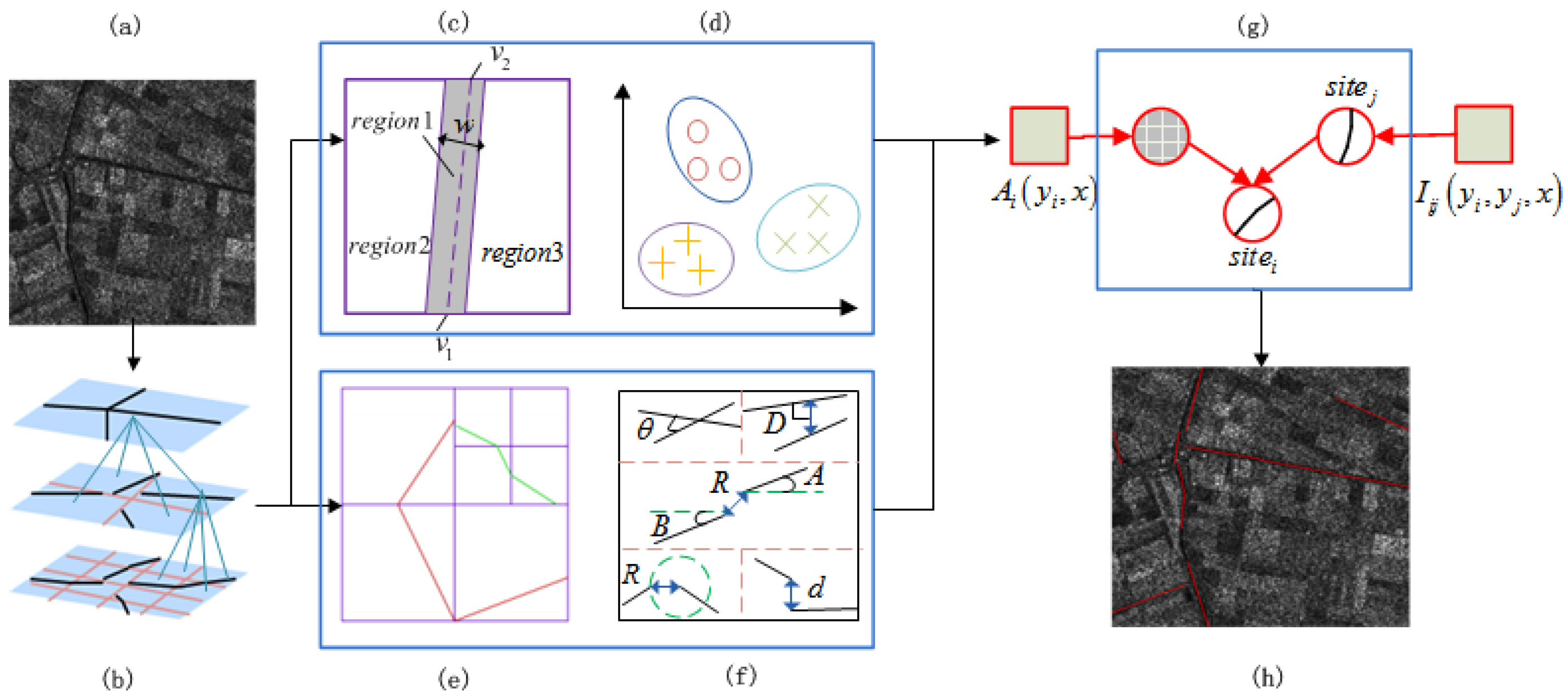
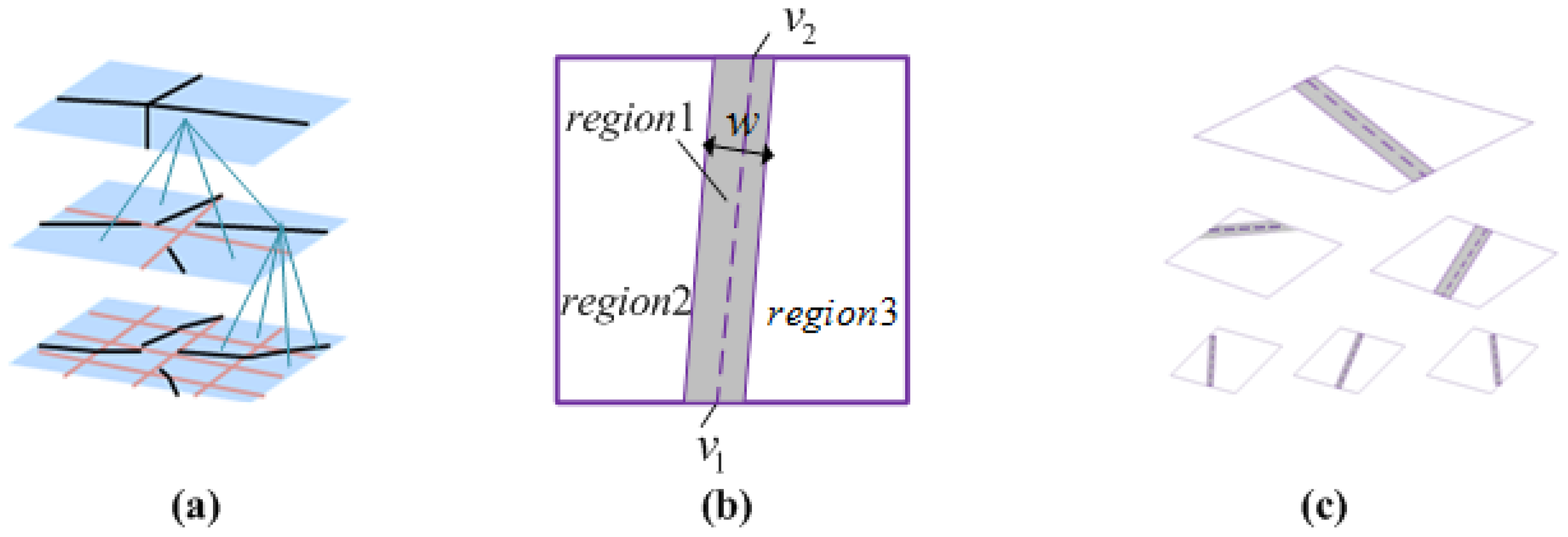
A multi-scale analysis is introduced to construct image pyramids on the data of each look, in which each image is partitioned into a sequence of dyadic squares at each level.

(2)

Based on our previous work, multi-scale operators are used to obtain the likelihood and prior constraints in CRF: for the unary potential, a detector called the multi-scale linear feature detector (MLFD) computes the maximum responses of road segments in dyadic squares at different scales.

(3)

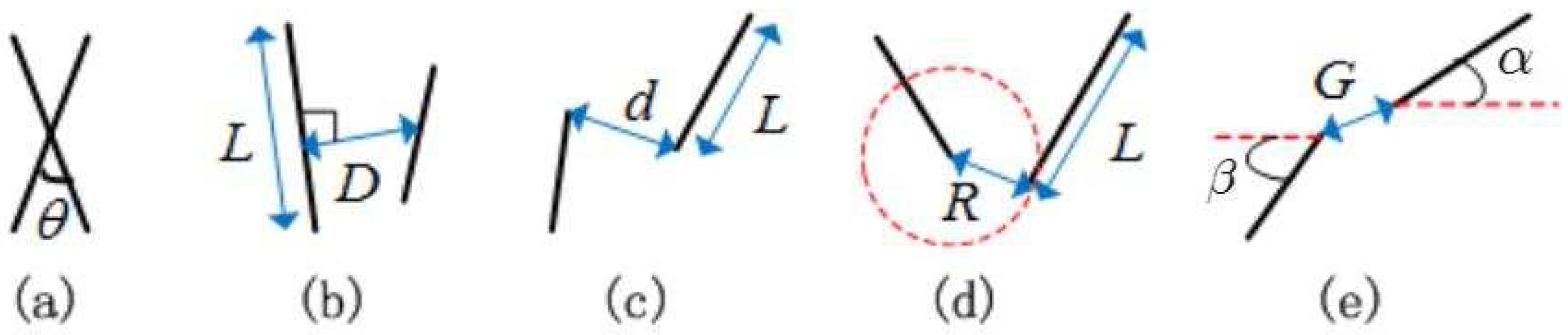
For the pairwise potential in the CRF, five constrained relationships, including distances and crossing angles between adjacent segments, are obtained under a beamlet framework, and several truncated linear functions are elaborately designed to avoid over-smoothing.

The remainder of this paper is structured as follows. The details of the Bayesian framework are presented in Section 2. Section 3 describes the unary potential in the CRF model, and Section 4 details the pairwise potential in the CRF model. Section 5 provides a summary, including the flowchart of the Bayesian framework. Finally, Section 6 presents an experiment based on airborne and spaceborne SAR data, and Section 7 presents the conclusion of this paper.

2. Bayesian Framework

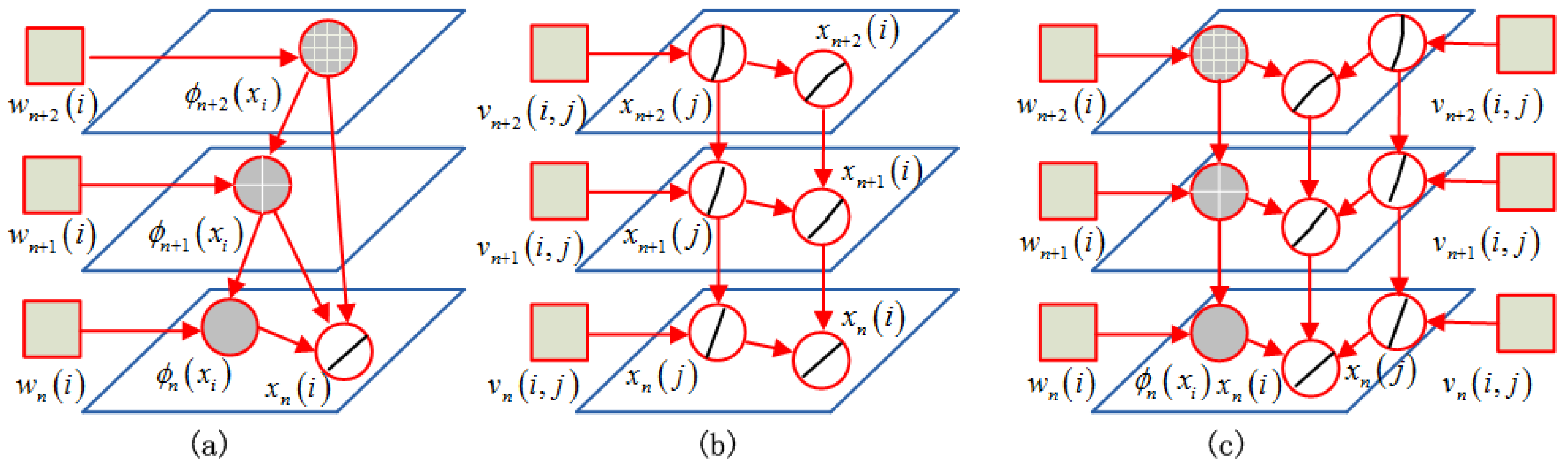
Road extraction can be considered to be a binary labeling problem, and many prior assumptions about roads may be encoded into models. In this paper, a Bayesian framework is utilized to transfer the road network extraction to joint reasoning of the likelihood of fraction extraction and the priority of network optimization. We construct a CRF model with elaborately-designed prior terms for road extraction from SAR images: (1) a multi-scale linear feature detector (MLFD) [14] provides the likelihood for road segments to acquire the sparse representation of road structures on multi-look data; (2) local priors are described with several constraints from the beamlet. The beamlet analysis [15,17] is a multi-scale framework for the detection of geometric objects, which employs a range of scale, localization and orientation line segments for image representation. Here, we provide the flowchart to present our framework in Figure 1. First, the MLFD framework is exploited to extract the likelihood of road segments using the multi-scale pyramid. Then, beamlet analysis and the prior distance constraints are incorporated to form the unary and pairwise terms in the CRF model. Finally, the Bayesian approach based on maximum a posteriori (MAP) [18] optimization is performed to obtain the road extraction results.

2.1. CRF Model

As a graph model, CRF can provide accurate decisions on classification results and compute the probability distribution of the labeled domain from the input samples. Compared with MRF, which models the joint probability distribution to optimize global information, CRF directly constructs the posterior probability distribution of the label field to deliver the association optimization of prior and likelihood information.

Let x denote the observed data and y be the label set (binary, $-1$ or one in this paper); the posterior probability can be represented in exponential form as:

$$P\left(y\right|x)\propto exp\left\{{\displaystyle \sum _{i\in S}}{A}_i(y_i,x)+{\displaystyle \sum _{i\in S}}{\displaystyle \sum _{j\in N_i}}{I}_{ij}\left(y_i,y_j,x\right)\right\}$$

(1)

$I=\left\{x_1,x_2,\dots ,x_M\right\}$ means that image I is composed of M pixels or superpixels $x_i$ (a collection of some pixels), where i represents a segment in $S=\left\{1,2,\dots ,M\right\}$ of all the image segments and j is a segment in the neighboring set $N_i$ of segment i. In Formula (1), $A_i$ and $I_{ij}$ are the unary and pairwise potentials, respectively. $A_i$ measures the probability of segment i taking label $y_i$, while $I_{ij}$ describes the interaction between segments i and j.

2.2. CRF Reasoning for Road Extraction

In addition to directly modeling the conditional distribution of labels, another key aspect of CRF in our view is that the observed samples, i.e, the road segments, in each dyadic segment do not have to be conditionally independent. Multi-scale approaches for CRF are widely applied in linear target detection [14,15,19], in which the features at each scale are different. By extracting features for every probable linear target scale and learning the parameters jointly across scales, we render the model scale invariant.

For road extraction applications, we flexibly configure two forms of feature functions in CRF: the state feature function ${\varphi }_i\left(x\right)$ of the label at segment i in the unary term and the transition feature function $\mu \left({\varphi }_i\left(x\right),{\varphi }_j\left(x\right)\right)$ of labels at segment i and an adjacent segment j in the pairwise term. The unary potential and the pairwise potential are designed with their respective classifiers. The state feature is intended to interpret road properties sparsely, where the maximum responses of the multi-scale dyadic segments in MLFD act as feature elements. The transition feature represents local geometric relationships between neighboring segments, such as the angular and endpoint distances. Therefore, the conditional probability $P\left(y|\varphi \left(x\right)\right)$ can be given by:

$$P\left(y|\varphi \left(x\right)\right)=\frac{1}{Z\left(\varphi \left(x\right)\right)}exp\left\{{\displaystyle \sum _{i\in S}}{A}_i\left(y_i,{\varphi }_i\left(x\right)\right)+{\displaystyle \sum _{i\in S}}{\displaystyle \sum _{j\in N_i}}{I}_{ij}\left(y_i,y_j,\mu \left({\varphi }_i\left(x\right),{\varphi }_j\left(x\right)\right)\right)\right\}$$

(2)

where $Z\left(\varphi \left(x\right)\right)$ is the partition function and is defined by:

$$\begin{array}{c}\hfill \begin{array}{c}\hfill Z\left(\varphi \left(x\right)\right)={\displaystyle \sum _y}exp\left\{{\displaystyle \sum _{i\in S}}{A}_i\left(y_i,{\varphi }_i\left(x\right)\right)+{\displaystyle \sum _{i\in S}}{\displaystyle \sum _{j\in N_i}}{I}_{ij}\left(y_i,y_j,\mu \left({\varphi }_i\left(x\right),{\varphi }_j\left(x\right)\right)\right)\right\}\end{array}\end{array}$$

(3)

In the CRF graph structure conditioned on observation segment $x_n\left(i\right)$ (see Figure 2), $x_n\left(i\right)$ is the candidate segment in segment i at scale k, $x_n\left(j\right)$ is a segment interacting with $x_n\left(i\right)$ and ${\varphi }_n\left(x_i\right)$ is the likelihood feature generated by a specified partition degree at scale n. We take the random variable $x_e$ to be a vertex in the CRF graph; its label $y_e$ will be one when it actually lies on road lines.

3. Unary Potential in Our CRF Model

The multi-scale linear feature detector (MLFD) captures the unary potential, in which the maximum responses of multi-scale dyadic segments act as feature elements.

The unary potential function $A_i\left(y_i,{\varphi }_i\left(x\right)\right)$ describes the information in a single segment and measures the probability that the label of segment i is $y_i$ for the observed data x. Different CRFs may take various classifiers as unary potentials, such as boosting potential [17] and kernel CRF [15]. In this CRF, our unary potential is defined by the general logistic classifier [20], and the likelihood features are given by the MLFD.

3.1. Likelihood Information from the MLFD

In [8], the multi-scale linear feature detector designs a mask filter that divides an image into several different regions to detect local region segments. The mask size range is selected using the multi-resolution method. The operator can adaptively adjust the mask size and change the width and direction of the central region. Additionally, the statistical and geometrical properties of local region are taken into account.

MLFD is derived from the fusion of the ratio line detector (D1) and the cross-correlation line detector (D2) [7]. During the MLFD procedure, an input image is iteratively partitioned into two by two squares, and then, a quadtree for the image pyramid is constructed, as shown in Figure 3a. At each level, the MLFD computes the responses of all previously-partitioned segments. The responses are regarded as features, and the association of features at different levels is considered to be the feature vector in the likelihood term of the CRF framework. In detail, the mask partitions a local segment into three adjacent regions (see Figure 3b); then, the local segment response can be expressed as $r\left(v_1,v_2,w,{\mu }_1,{\mu }_2,{\mu }_3\right)$, where $v_1,v_2$ are the endpoints of the central line in the central area, w is the width of the central area and ${\mu }_1,{\mu }_2,{\mu }_3$ are the mean values of the three regions in the mask, which are calculated using the following equation:

$${\mu }_i=\left(1/n_i\right){\displaystyle \sum _{s\in i}}{A}_s$$

(4)

where s is a pixel with amplitude $A_s$ and $n_i$ counts the number of pixels in the single segment i.

With l denoting the length of the central area and α expressing the uniformity coefficient, the MLFD response can be defined as:

$$T\left(m\right)=\frac{l\alpha r\rho }{1-r-\rho -2r\rho },r,\rho \in \left[0,1\right]$$

(5)

where m is the mask central line in the area to be detected and r and ρ are the responses of the D1 and D2 operators, respectively, as given in Equation (6). α evaluates the continuity of the central region that is related to r.

$$\left\{\begin{array}{c}r=min\left(r_{12},r_{13}\right)\\ r_{ij}=1-min\left({\mu }_i/{\mu }_j,{\mu }_j/{\mu }_i\right)\\ \alpha =\left(1-r_{12}\right)\times \left(1-r_{23}\right)\end{array}\right.,\left\{\begin{array}{c}\rho =min\left({\rho }_{12},{\rho }_{13}\right)\\ {\rho }_{ij}^2=1/\left(1+\left(n_i+n_j\right)\frac{n_i{\gamma }_i^2{c}_{ij}^2+n_j{\gamma }_j^2}{n_i{n}_j{\left(c_{ij}-1\right)}^2}\right)\end{array}\right.$$

(6)

where $r_{ij}$ denotes the ratio response of regions i and j, $c_{ij}={\mu }_i/{\mu }_j$ and ${\gamma }_i$ is the variance of the amplitudes in region i.

In this paper, with SAR data, we can obtain three different MLFD responses $T^K\left(m\right)$ about different looks, i.e., $K\in \{hh,hv,vv\}$. $T^K\left(m\right)$ is a concatenated vector consisting of responses on three scattering elements, where $A_s^{hh}$ is the amplitude of scattering element $S_{hh}$. The responses $T^K\left(m\right)$ will be designed into the state feature function and the transition feature function in CRF.

3.2. Unary Potential Term

In this paper, we take a general logistic classifier to describe the unary potential in CRF, i.e.,

$$\left\{\begin{array}{c}{A}_i\left(y_i,{\varphi }_i\left(x\right)\right)=log\left(1+e^{-y_i{\mathit{\omega }}^T{h}_i\left(x\right)}\right)\\ h_i\left(x\right)={\left[T_1\left(m_i\right),T_2\left(m_i\right),\dots ,T_n\left(m_i\right),1\right]}^T\end{array}\right.$$

(7)

where $h_i\left(x\right)$ is the multi-scale feature matrix of dyadic segment i, which consists of the MLFD responses. $T_n\left(m_i\right)$ denotes the maximum MLFD response in segment i at scale n. The model parameter vector $\mathit{\omega }={\left[{\omega }_1,{\omega }_2,\dots ,{\omega }_K,{\alpha }_1\right]}^T$ contains a weight for each item in the matrix $h_i\left(x\right)$ and is learned during the training process, and ${\alpha }_1$ is a trade-off parameter.

4. Pairwise Potential in Our CRF Model

The pairwise potential function $I_{ij}\left(y_i,y_j,\mu \left({\varphi }_i\left(x\right),{\varphi }_j\left(x\right)\right)\right)$ reflects the spatial interaction between two segments i and j regarding the entirety of the observed data x. The difference with clique potentials in MRFs is that segment j does not necessarily have to be in the neighborhood of segment i, but may be an arbitrary segment from all of the data. In the road extraction framework, the prior information in the pairwise potential is exploited under beamlet analysis. We fully utilize the design flexibility of the feature matrix in the pairwise potential and introduce several constraints between local neighboring segments. The pairwise potential function is designed with prior constraints, including segment length, curvature and intersection distance.

4.1. Prior Constraints under Beamlet Analysis

Beamlet analysis [21] is a multi-resolution image understanding framework, which was developed by Donoho and Hou in 2000. It localizes scale, location and orientation based on dyadically-organized line segments. In this framework, a beamlet transform is performed based on the beamlet dictionary, which consists of all types of line segments at a range of scales, locations and orientations; then, the beamlet pyramid and graph can be constructed for the beamlet algorithm.

Beamlet transform is accomplished through a multi-scale decomposition similar to MLFD that iteratively divides an image into a series of dyadic segments. In each segment, a connection of two arbitrary vertices will form a beamlet segment. The summation of the grey-level values of pixels on a beamlet is defined as a beamlet transform, and the discrete beamlet transform response in this paper is given by:

$$T\left(b\right)={\displaystyle \sum _{p\in b}}g\left(p\right)/l{\left(b\right)}^{1/2}$$

(8)

where $g\left(p\right)$ is the gray-level value of pixel p and the length $l\left(b\right)$ counts the number of pixels in segment b.

Furthermore, during beamlet analysis, a multi-scale partition is used to acquire a sequence of dyadic segments $\mathit{P}$ at different levels. Each square is represented by a beamlet, and the beamlet decomposition to depict the best partition is:

$$p_{opt}=arg{\displaystyle \underset{p\in \mathit{P}}{max}}\left\{{\displaystyle \sum _{s\in p}}{\displaystyle \underset{b\sim s}{max}}T\left(b\right)-\lambda \#p\right\}$$

(9)

where $b\sim s$ is the beamlet mask b on dyadic segment s and $\#p$ counts the number of units in set p at a certain level. Parameter λ is the complexity-penalized coefficient that measures the decomposition degree. A smaller λ will obtain many more segments and show more image detail, whereas a large λ may determine global outlines in the image with fewer noise segments.

To obtain the optimal solution for Equation (9), a bottom-up pruning process is employed for the constructed quadtree. For one segment at different scales, only the segments of maximum responses at one level are retained:

$${\displaystyle \sum _{i=1}^4}T\left(b_i\right)-4\lambda >T\left(b_p\right)-\lambda$$

(10)

where the segments of four sub-squares will be saved and the response of their parent will be updated into the sum of four sub-responses; otherwise, the sub-squares are discarded, and their parent will no longer be subdivided. In Equation (10), $T\left(b_i\right)$ is the beamlet response of the i-th sub-square, and $T\left(b_p\right)$ is their corresponding parent square. In this pruning phase, the final road results of the beamlet are offered.

Perceptual organization, which is known to assess the structural relationships of various primitive elements, has been widely used in computer vision [22,23]. In this study, the contextual relationships between road segments, such as the intersection angles, curvatures, endpoint distances and proximities, provide global optimization with effective prior constraints for road extraction from SAR images. We use several relational constraints to group and label segments, as shown in Figure 4.

Angular distance: This item measures the crossing angle of two lines (see Figure 4a) and is defined as:

$$D^a=min\left(\theta ,\pi -\theta \right)$$

(11)

where ${\theta }_1$ and ${\theta }_2$ are the tangent angles of two segments with the value range $\left(\left.-\pi /2,\pi /2\right]\right.$.

Lateral distance: The lateral distance of segments in a local region should be small, and it is computed as the perpendicular distance from the midpoint of the shorter line to that of the longer one. As shown in Figure 4b, if L denotes the length of the longer segment and D is the vertical distance of these two lines, then the lateral distance is given by:

$$D^t=D/L$$

(12)

Endpoint distance: This is similar to the lateral distance, with d representing the minimum intersection distance of four endpoints in the two lines and L denoting the length of the longer segment, as shown in Figure 4c. The endpoint distance can be written as:

$$D^e=d/L$$

(13)

Proximity: The proximity of two segments measures how likely it is that adjacent segments are close to each other, and it reflects their perceptual significance, as shown in Figure 4d. The proximity is calculated by:

$$P=L^2/2\pi R^2$$

(14)

where L is the length of the shorter line and R is the minimum intersection distance similar to d in Equation (13).

Continuity: Continuity [23] describes the structural relationship among segments and determines the weight by which road segments should be connected, as shown in Figure 4e. Continuity is defined as:

$$C=\frac{1}{\left({\alpha }^2+{\beta }^2\right)\left(w_1+w_{2}R\right)}$$

(15)

where α and β are the intersection angles of lines with horizontal lines at joined endpoints and $w_1$ and $w_2$ determinate the weight of the smoothness at the joined endpoint and the distance between connecting endpoints. Similar to MLFD responses $T^K\left(m\right)$ on SAR data, the above five constraints are computed on SAR dataset K and combined into five vectors with three elements. The vectors are written as $D_K^a$, $D_K^t$, $D_K^e$, $P^K$ and $C^K$. In the final pairwise potential, the first three vectors constitute the smoothness prior, and the last two form the contrast-dependent prior.

4.2. Pairwise Potential Term

Our pairwise potential consist of a smoothness prior and contrast-dependent prior. Considering the extension and smoothness of roads, $D^a$, $D^t$ and $D^e$ between segments in the local region are extremely small, which means that a smaller value of this smoothness prior will enforce a higher energy and that we should strongly penalize a larger distance of $D^a$, $D^t$ and $D^e$. We introduce a sigmoid function for the smoothness prior as follows:

$${\psi }_{ij}^s=\left\{\begin{array}{cc}\frac{1}{1+exp\left(\mathit{\vartheta }\odot \left({\mu }_{ij}^s\left(x\right)-\mathit{\kappa }\right)\right)}{v}_{sij},\hfill & if{y}_i=y_j\\ 0,\hfill & otherwise\end{array}\right.$$

(16)

where ${\mu }_{ij}^s\left(x\right)=[D_K^a,D_K^t,D_K^e]$ is the associated feature vector of segments i and j on SAR dataset K; $\mathit{\vartheta }$ and $\mathit{\kappa }$ are the curve inflexion vectors for $D^a$, $D^t$ and $D^e$; ⊙ denotes the Hadamard product; $v_{sij}$ measures the influence of each distance on the smoothness prior.

Along rather continuous roads, adjacent segments have similar angular and endpoint distances, and these parameters of actual road segments will be close to the mean vector of the local candidates’ set. We obtain a local set that contains at least ten segments in the neighboring region of segment $x_i$, and then, we compute the mean feature vector ${\overline{\mu }}_i$ and standard deviation ${\sigma }_i$. With the Euclidean distance, $d_{ij}={\mu }_{ij}-{\overline{\mu }}_i$ measures the deviation of vector ${\mu }_{ij}$ from ${\overline{\mu }}_i$, and the weight $v_{sij}$ is defined as:

$$v_{sij}=\left\{\begin{array}{ccc}{v}_{sij},\hfill & if\hfill & d_{ij}\le {\sigma }_i\hfill \\ v_{sij}\left(1-d_{ij}/\left(4{\sigma }_i\right)\right),\hfill & if\hfill & {\sigma }_i<d_{ij}\le 4{\sigma }_i\hfill \\ 0,\hfill & if\hfill & d_{ij}>4{\sigma }_i\hfill \end{array}\right.$$

(17)

The truncated linear function [13] ensures a full weight to pairwise segments within ${\sigma }_i$, a linearly decreasing weight to segments between ${\sigma }_i$ and $4{\sigma }_i$ (an empirical threshold) and removes the pairwise segments above four standard deviations. The weighting function significantly helps to avoid over-smoothing.

Then, the contrast-dependent prior within the Ising model [24] takes the following form:

$${\psi }_{ij}^p=y_i{y}_j{\mu }_{ij}^p\left(x\right)v_{pij}^T$$

(18)

where ${\mu }_{ij}^p\left(x\right)=[f_{ij}\left(x\right),P_{ij},C_{ij}]$ is the associated feature vector, $f_{ij}=[h_i\left(x\right),h_j\left(x\right)]$ is a concatenation feature of single segments i and j; $P_{ij}$ and $C_{ij}$ represent the proximity and continuity priors, respectively; and $v_{pij}^T$ denotes the weights for ${\mu }_{ij}^p\left(x\right)$, which are tuned during the CRF training process.

Finally, the pairwise potential in this CRF model is defined as:

$$I_{ij}(y_i,y_j,x)=\epsilon {\psi }_{ij}^s+\eta {\psi }_{ij}^p$$

(19)

where ε and η trade-off the strengths of pairwise terms against the unary term in the model and will be set via finding the optimal value on the training set. The optimization process of Equation (2) is employed with an improved version of the quasi-Newton method based on the version provided by Gould et al. [25].

5. Post Processing

5.1. The Complete Posterior Distribution of CRF

Using the concrete definitions of the unary potential in Equation (7) and pairwise potential in Equation (19), the posterior probability $p\left(y|\varphi \left(x\right)\right)$ in Equation (1) can be rewritten as:

$$p\left(y|\varphi \left(x\right),\mathrm{\Theta }\right)\propto {\displaystyle \prod _{i\in S}}\left(1+exp\left(-y_i{\mathit{\omega }}^T{h}_i\left(x\right)\right)\right)\times {\displaystyle \prod _{i\in S}}{\displaystyle \prod _{j\in N_i}}\left(y_i{y}_j{\mathit{v}}^T{\mu }_{ij}\left(x\right)\right)$$

(20)

where $\mathrm{\Theta }=\left\{\mathit{\omega },\mathit{v}\right\}$ is the set of parameters in the model.

5.2. Normalization Methods

In the above sections, we have defined various features and prior constraints. These can be used to interpret different properties and provide a uniform description of the characteristics of roads. To avoid numerical instability in the CRF training period, normalization methods should be introduced into the handling of the feature matrices.

Binarization: A binarization method is used for the angular distance $D^a$, the lateral distance $D^t$ and the endpoint distance $D^e$ in this study. The binarization is performed by comparing the segment feature values with its four-connection neighborhood. Taking the angular distance $D_{ij}^a$ of segments in segments i and j as an example, $D_{ij}^a$ is calculated using Equation (11), and the average angular distance ${\overline{D}}_i^a$ between segment i and its neighborhood is defined by:

$${\overline{D}}_i^a={\displaystyle \sum _{k\in N_i}}{D}_{ik}^a/num\left(N_i\right)$$

(21)

where $N_i$ is the neighborhood collection of segment i, $D_{ik}^a$ is the angular distance of segments in segments i and k and $num\left(N_i\right)$ counts the quantity of set $N_i$.

Considering the extension and smoothness of roads, $D^a$, $D^t$ and $D^e$ between segments in local regions should have small values; thus, we set threshold $T_a$ using several sets of experimental results. In particular, the angular distance $D_{ij}^a$ will be retained if the absolute difference from the local average ${\overline{D}}_i^a$ is smaller than threshold $T_a$; otherwise, it will be discarded. Therefor, the binarization is written as:

$$D_{ij}^{a\left(b\right)}=\left\{\begin{array}{cc}1,& if|D_{ij}^a-{\overline{D}}_i^a|\le T_a\\ 0,& if|D_{ij}^a-{\overline{D}}_i^a|>T_a\end{array}\right.$$

(22)

Similar to Equation (22), the binarizations for the lateral distance $D_{ij}^t$ and the endpoint distance $D_{ij}^e$ can be obtained by substituting the absolute difference with the ratio between the feature value and the local average. For the thresholds, we define these two binarizations as:

$$D_{ij}^{t\left(b\right)}=\left\{\begin{array}{c}1,\begin{array}{cc}& if{D}_{ij}^t/{\overline{D}}_i^t\le T_t\end{array}\\ 0,\begin{array}{cc}& if{D}_{ij}^t/{\overline{D}}_i^t>T_t\end{array}\end{array}\right.\begin{array}{cc};& D_{ij}^{e\left(b\right)}=\left\{\begin{array}{c}1,\begin{array}{cc}& if{D}_{ij}^e/{\overline{D}}_i^e\le T_e\end{array}\\ 0,\begin{array}{cc}& if{D}_{ij}^e/{\overline{D}}_i^e>T_e\end{array}\end{array}\right.\end{array}$$

(23)

For the proximity $P_{ij}$ and the continuity $C_{ij}$, the post-processing is normalized as the ratio of the current value and the local average, but not the binarizations, and can be expressed as:

$$\left\{\begin{array}{c}{P}_{ij}^{\left(b\right)}=P_{ij}/{\overline{P}}_{ij}\hfill \\ C_{ij}^{\left(b\right)}=C_{ij}/{\overline{C}}_{ij}\hfill \end{array}\right.$$

(24)

where the local averages ${\overline{P}}_{ij}$ and ${\overline{C}}_{ij}$ are calculated using the same method as for ${\overline{D}}_i^a$ in Equation (21).

Finally, the association feature matrix ${\mu }_{ij}\left(x\right)$ in the pairwise potential can be determined using the five binary prior constraints given above and the features of segments i and j. Then, the definite form is as follows:

$${\mu }_{ij}\left(x\right)=\left[f_{1ij},f_{2ij},\cdots ,f_{nij},D_{ij}^{a\left(b\right)},D_{ij}^{t\left(b\right)},D_{ij}^{e\left(b\right)},P_{ij}^{\left(b\right)},C_{ij}^{\left(b\right)}\right]$$

(25)

where $f_{nij}=\left[h_{ni}\left(x\right),h_{nj}\left(x\right)\right]$ is a simple concatenation of the features of single segments i and j at a particular scale n.

6. Experiments and Results

6.1. Experimental Data and Settings

To evaluate the proposed road extraction method, both spaceborne and airborne SAR images are used to test the method. The first two data are real spaceborne TerraSAR data acquired in Germany (see Figure 5a) and Wuhan, China (see Figure 6a). The size of the first image is $1000\times 1000$ pixels, and its spatial resolution is $3.0$ m$\times 2.2$ m. The second image is a wide scene with a size of $1152\times 644$ pixels. The corresponding ground truths are two-dimensional images labeled manually (Figure 5b and Figure 6b). We also used airborne SAR data, acquired using equipment developed by China and derived from airborne X-band SAR provided by the 38th Institute of China, Electronics Technology Company, to assess the proposed method. The test area is near Lingshui County, Hainan Province, China. The span images are presented in Figure 7a and Figure 8a, and their sizes are both $1000\times 1000$ pixels. The parameters for each experiment, learned during the training process, are listed as follows: in Figure 5, the decomposition degree λ of the beamlet is set as 4.4, and the curve inflexion vectors are $\mathit{\vartheta }$ = [1,5,7] and $\mathit{\kappa }$ = [30, 0.8, 0.5], whereas in Figure 6, λ is 2.3, $\mathit{\vartheta }$ = [1,6,5] and $\mathit{\kappa }$ = [20, 0.8, 0.7]. For the airborne SAR scenes in Figure 7a and Figure 8a, the comparative methods MLFD and beamlet are implemented on the span images, and the decomposition degrees λ are 4.6 and 5.3, respectively. The CRF parameters, curve inflexion vectors $\mathit{\vartheta }$ and $\mathit{\kappa }$ are concatenated by parameters from the original SAR dataset. In Figure 7, $\mathit{\vartheta }$ = [1.2, 4, 6, 1.8, 4.5, 6.3, 1.5, 4.2, 6.5] and $\mathit{\kappa }$ = [22, 0.7, 0.75, 26, 0.74, 0.8, 24, 0.71, 0.78], whereas in Figure 8, $\mathit{\vartheta }$ = [1.5, 5.1, 7.5, 2.1, 5.8, 8, 1.7, 5.3, 7.7] and $\mathit{\kappa }$ = [32, 1, 1.2, 36, 1.4, 1.7, 33, 1.2, 1.4].

Several metrics have been proposed to qualitatively evaluate the performance of road extraction. In general, there are three such metrics for evaluation [23], which are defined as:

$$\left\{\begin{array}{c}\mathrm{completeness}=L_r/L_{gt}\hfill \\ \mathrm{correctness}=L_r/L_N\hfill \\ \mathrm{quality}=L_r/(L_N+L_{ugt})\hfill \end{array}\right.$$

(26)

where the completeness means the proportion of the ground truth length ($L_{gt}$) that is extracted exactly, $L_r$ is the matching length between the extracted roads and the ground truth and the correctness ($L_r/L_N$) represents the fraction of total extracted road length ($L_N$) that matches the actual roads. The quality is given by $L_r/(L_N+L_{ugt})$, with $L_{ugt}$ being the length of actual roads that are not matched by the extracted roads. If the midpoint distance between the extracted roads and the reference roads is less than a given tolerance, then we consider that the extracted roads match actual roads. The tolerances in these four images are set as 13, 8, 11 and 13 pixels.

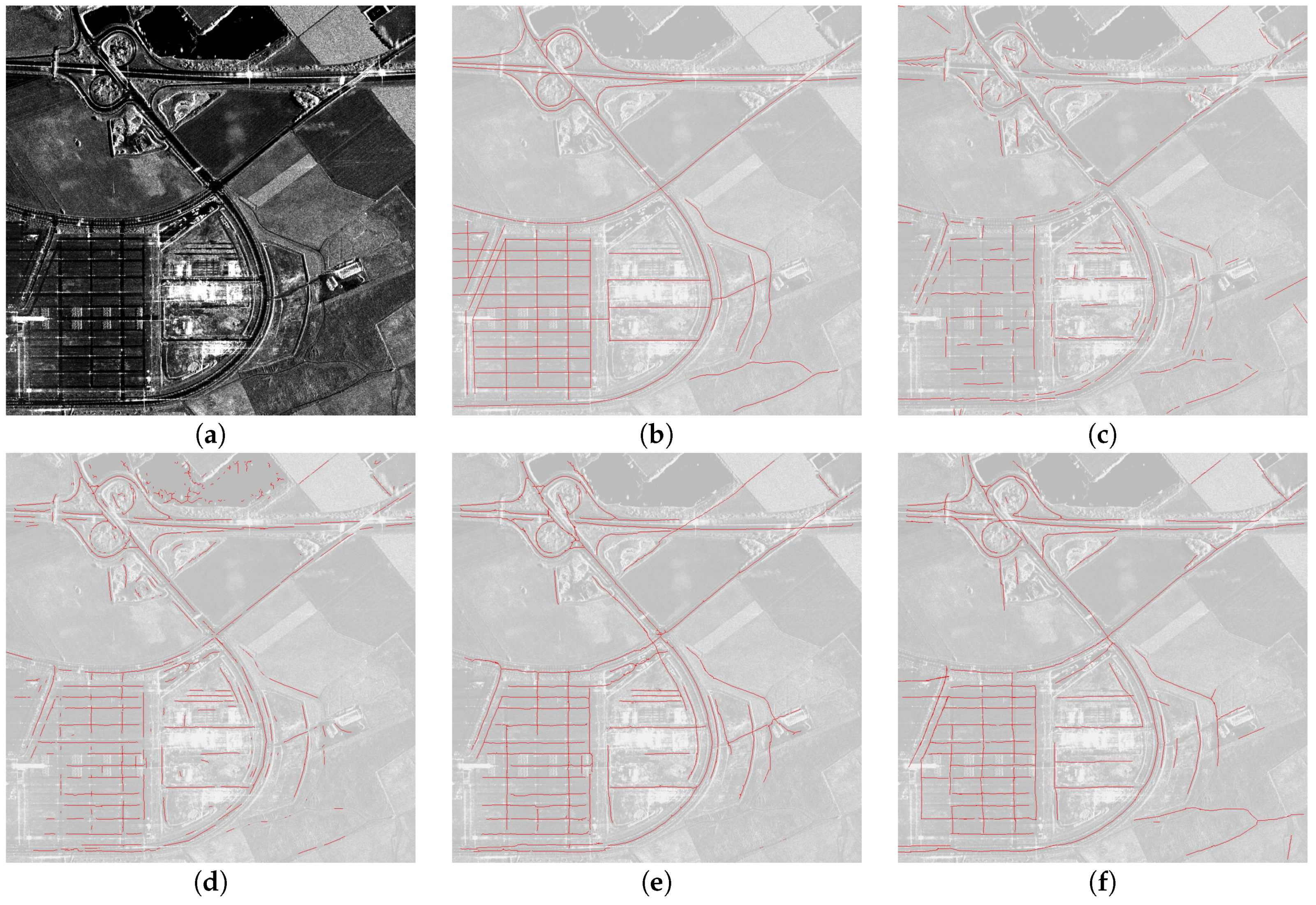
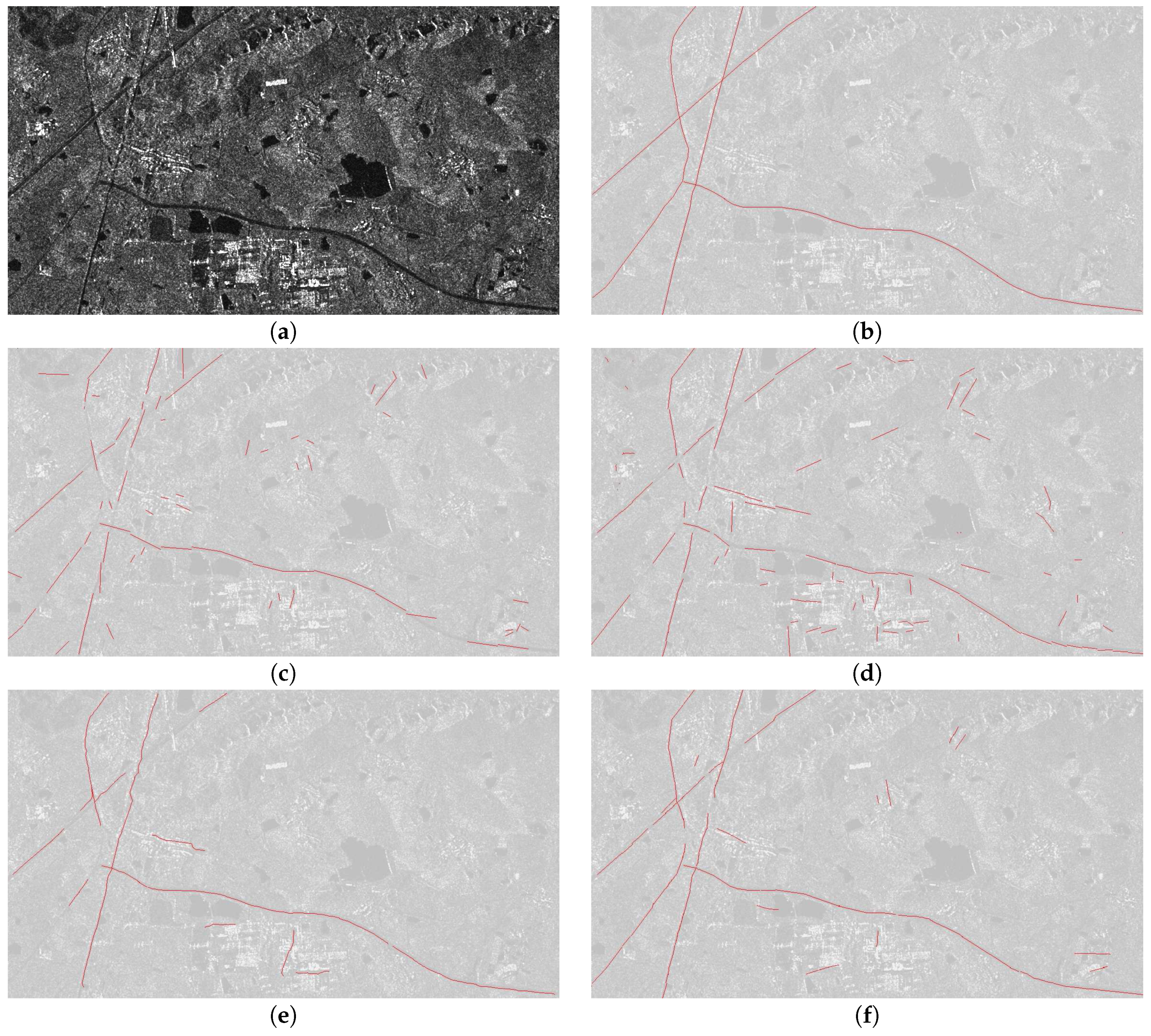
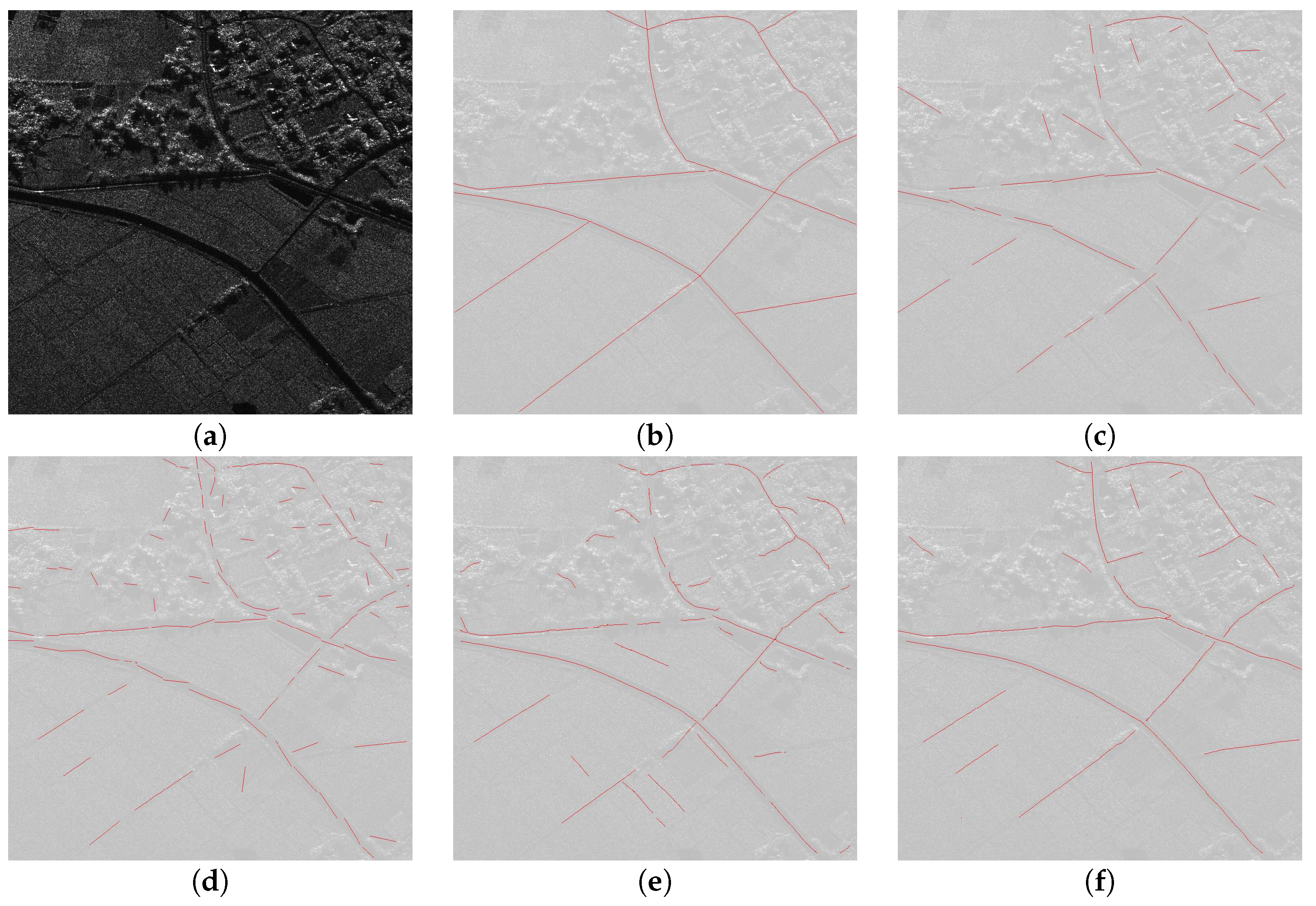
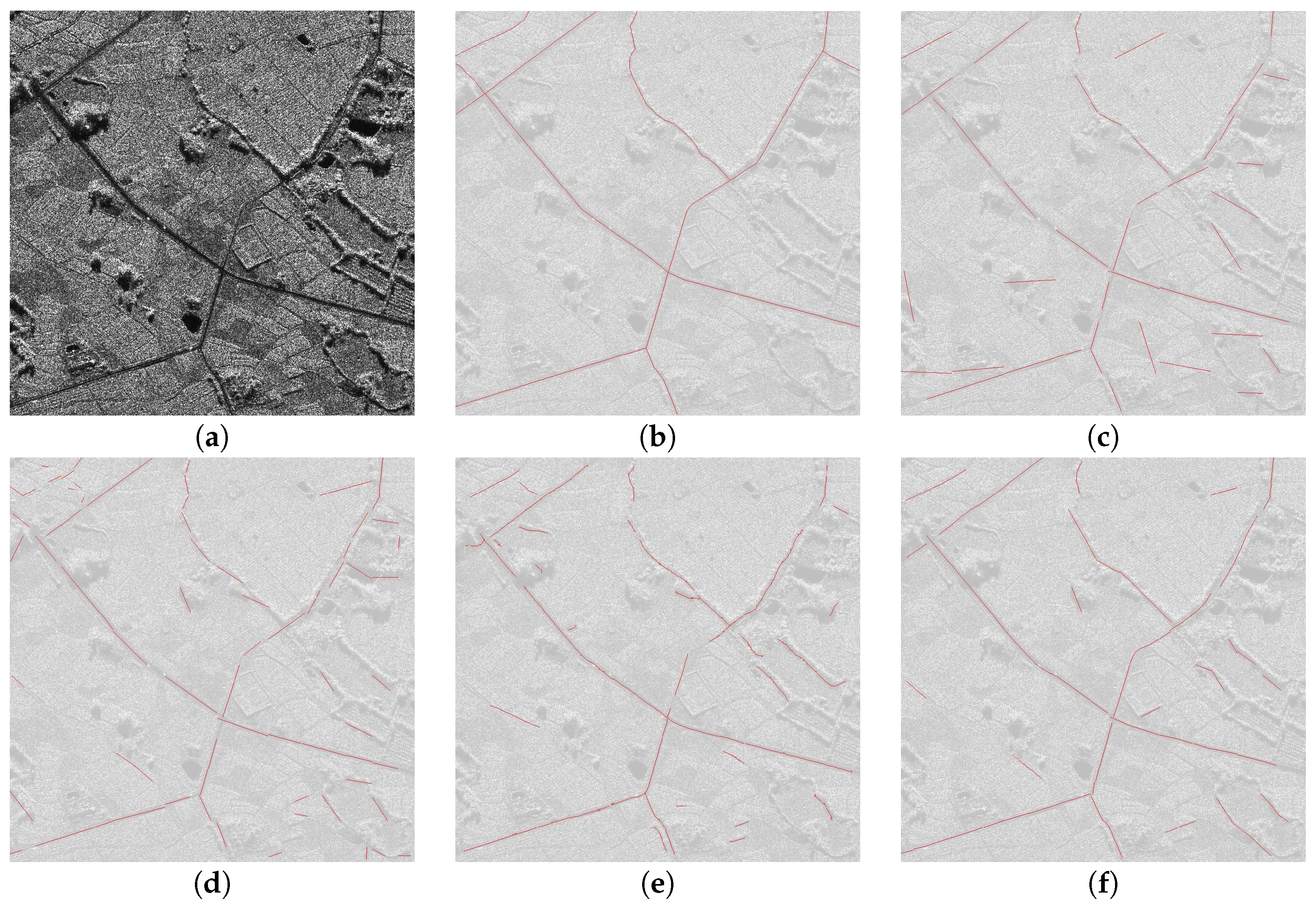
6.2. Experimental Results

Experiments of the proposed methodology and several comparative experiments are conducted using real spaceborne SAR and airborne SAR images. For Terra-SAR spaceborne data, Figure 5c and Figure 6c show the detected road segments using MLFD. This method primarily finds the overall road outlines with relatively little noise generation, but MLFD cannot handle the complex road intersections very well, as is obvious in the first image. Figure 5d and Figure 6d are the results of beamlet decomposition, which contain more road details and sophisticated segments even in complex areas and intersections; however, this produces many more non-road segments in local neighboring areas. Figure 5e and Figure 6e are the road networks after global optimization by MRF of Tupin [8], which connects adjacent long segments into lines when neglecting short ones by setting a certain length. However, it fails to extract such lines in dense urban areas where roads are of a short length and complex surroundings, and particularly in the second dataset that contains minor road segments, MRF mistakenly discards some positive short segments. The results of the CRF model are presented in Figure 5f and Figure 6f, which follow the entire outline extracted by MLFD and preserve the elaborate details in complex scenes extracted by beamlet when noise is greatly removed. Compared to MRF, many new segments are created, and the road lines are very smooth.

For airborne SAR data, comparative results are obtained on the span images. Figure 7c and Figure 8c present the roads of MLFD, where the segments are discontinuous fragments. However, when less non-roads are reserved, the MLFD method obtains the effective segments along actual lines. The beamlet results are shown in Figure 7d and Figure 8d, in which more complete fragments are obtained as a whole and more refined segments along curves and crossroads than MLFD. The optimized roads of MRF are given in Figure 7e and Figure 8e, where we can observe that most road lines match real roads and are connected especially along the crossroad, but some segments are misleading around complex building areas. The fusion results of the proposed CRF algorithm are presented in Figure 7f and Figure 8f, where new segments are selected, and then, the adjacent roads are jointed smoothly; moreover, the extremely small noise is greatly reduced. Both MRF and CRF retain some pseudo-roads, such as roofs and splitting lines between farmlands.

To evaluate the effect of the unary potential and pairwise potential in the proposed method, the TerraSAR data are taken as an example for comparison. As shown in Figure 9c, there is an apparent presence of noise in the results of the unary potential alone. In other words, the labels of neighboring pixels are not consistent with each other. This is because the spatial relationships, namely the prior constraints, are not taken into account in this model. By contrast, better results are achieved by the fusion CRF model, which are shown in Figure 9d, since more contextual information is exploited to facilitate robust and effective road extraction.

Table 1. Comparisons of evaluation indices and time cost(s).

Data	Methods	Correctness	Completeness	Quality	Time Cost
Figure 5	MLFD	0.6341	0.4262	0.3692	5.7
	beamlet	0.6791	0.6092	0.4730	6.4
	MRF	0.7311	0.7107	0.5635	4.9
	CRF	0.7658	0.7495	0.6097	10.2
Figure 6	MLFD	0.6747	0.7271	0.5384	4.1
	beamlet	0.5358	0.6821	0.4590	4.6
	MRF	0.7288	0.8196	0.6614	3.2
	CRF	0.7744	0.8978	0.7117	8.4
Figure 7	MLFD	0.6725	0.5674	0.4446	4.7
	beamlet	0.5799	0.6199	0.4278	5.3
	MRF	0.7256	0.7982	0.6048	4.1
	CRF	0.7534	0.7719	0.7157	12.3
Figure 8	MLFD	0.5823	0.6824	0.4581	5.1
	beamlet	0.6452	0.7440	0.5280	5.6
	MRF	0.7697	0.7856	0.6397	4.7
	CRF	0.7952	0.8056	0.7279	13.4

presents comparisons of quality evaluations for each method on the test images. As shown in this table, MLFD has an acceptable correctness, but unsatisfactory completeness and quality, whereas beamlet possesses a higher completeness and quality because of showing more extracted details. The three indices of CRF increase markedly in both images. It is also apparent that the quality indices, which illustrate the overall assessment and the correctness index, are both the highest for CRF. As belief messages are passed among all of the image sites and several constraints are involved, the time cost of CRF is more expensive than that of MRF, but it is on the same scale. Because MRF deletes isolated short segments and concatenates adjacent segments into lines according to several rules, it has acceptable evaluation indices for all images.

7. Conclusions

In this paper, a Bayesian framework that combines multi-scale geometric detection operators and its application to road extraction from SAR images are presented. (1) The main contribution of this paper is the introduction of two road detection methods for multi-scale analysis and fusing them using a Bayesian framework to fully utilize the strengths of multi-scale analysis. The association optimization of CRF leads to a better road network compared with the separate detection methods. The grouped road network from CRF incorporates the best features of each method. In particular, MLFD guides the overall road outline and generates relatively little noise, whereas beamlet provides sophisticated segments even in complex areas and intersections. (2) In the CRF model, MLFD provides the multi-scale likelihood features for each dyadic segment, and the prior constraints are obtained under beamlet analysis. The learning and inference algorithm in a uniform pyramid structure guarantees finding joint global optimal results. (3) The experimental results show that the proposed fusion method for road extraction in SAR images markedly improved in correctness and quality compared with each independent operator and the optimization approach based on MRF, which verifies the effectiveness of our fusion methodology using CRF.

References

1. He, C.; Li, S.; Liao, Z.X.; Liao, M.S. Texture classification of PolSAR data based on sparse coding of wavelet polarization textons. IEEE Trans. Geosci. Remote Sens. 2013, 8, 4576–4590. [Google Scholar] [CrossRef]
2. Cheng, J.; Gao, G.; Ku, Y.; Sun, J.Y. Review of road network extraction from SAR images. J. Image Graph. 2013, 18, 11–23. [Google Scholar]
3. Canny, J. A computational approach to edge detection. IEEE Trans. Pattern Anal. Mach. Intell. 1986, 6, 679–698. [Google Scholar] [CrossRef]
4. Chanussot, J.; Mauris, G.; Lambert, P. Fuzzy fusion techniques for linear features detection in multitemporal SAR images. IEEE Trans. Geosci. Remote Sens. 1999, 37, 1292–1305. [Google Scholar] [CrossRef]
5. Touzi, R.; Lopes, A.; Bousquet, P. A statistical and geometrical edge detector for SAR images. IEEE Trans. Geosci. Remote Sens. 1988, 26, 764–773. [Google Scholar] [CrossRef]
6. Stoica, R.; Descombes, X.; Zerubia, J. A Gibbs point process for road extraction from remotely sensed images. Int. J. Comput. Vis. 2004, 57, 121–136. [Google Scholar] [CrossRef]
7. Negri, M.; Gamba, P.; Lisini, G.; Tupin, F. Junction-aware extraction and regularization of urban road networks in high-resolution SAR images. IEEE Trans. Geosci. Remote Sens. 2006, 44, 2962–2971. [Google Scholar] [CrossRef]
8. Tupin, F.; Maitre, H.; Mangin, J.; Nicolas, J.; Pechersky, E. Detection of linear features in SAR images: Application to road network extraction. IEEE Trans. Geosci. Remote Sens. 1998, 36, 434–453. [Google Scholar] [CrossRef]
9. Wegner, J.; Hansch, R.; Thiele, A.; Soergel, U. Building Detection From One Orthophoto and High-Resolution InSAR Data Using Conditional Random Fields. IEEE J. Sel. Top. Appl. Earth Obs. Remote Sens. 2011, 4, 83–91. [Google Scholar] [CrossRef]
10. He, X.; Zemel, R.; Carreira, M. Multiscale conditional random fields for image labeling. In Proceedings of the 2004 IEEE Computer Society Conference on Computer Vision and Pattern Recognition, Washington, DC, USA, 27 June–2 July 2004.
11. Huang, Z.; Xu, F.; Lu, L.; Nie, H. Object-based conditional random fields for road extraction from remote sensing image. In IOP Conference Series: Earth and Environmental Science; IOP Publishing: Bristol, UK, 2014; p. 012276. [Google Scholar]
12. He, C.; Shi, B.; Zhang, Y.; Su, X.; Yang, W.; Xu, X. The algorithm of building area extraction based on boundary prior and conditional random field for SAR image. In Proceedings of the IEEE International Geoscience and Remote Sensing Symposium-IGARSS, Melbourne, Australia, 21–26 July 2013; pp. 1321–1324.
13. Wegner, J.; Montoya-Zegarra, J.; Schindler, K. A higher-order CRF model for road network extraction. In Proceedings of the IEEE Conference on Computer Vision and Pattern Recognition, Portland, OR, USA, 23–28 June 2013; pp. 1698–1705.
14. He, C.; Liao, Z.; Yang, F.; Deng, X.; Liao, M. A novel linear feature detector for SAR images. Eurasip J. Adv. Signal Process. 2012, 2012, 1–9. [Google Scholar] [CrossRef] [Green Version]
15. He, C.; Liao, Z.; Yang, F.; Deng, X. Road Extraction From SAR Imagery Based on Multiscale Geometric Analysis of Detector Responses. IEEE J. Sel. Top. Appl. Earth Obs. Remote Sens. 2012, 5, 1373–1382. [Google Scholar]
16. Donoho, D. Wedgelets: Nearly minimax estimation of edges. Ann. Stat. 1999, 27, 859–897. [Google Scholar] [CrossRef]
17. Donoho, D.; Levi, O.; Starck, J.; Martinez, V. Multiscale geometric analysis for 3d catalogs. In Astronomical Telescopes and Instrumentation; International Society for Optics and Photonics: Waikoloa, HI, USA, 2002; pp. 101–111. [Google Scholar]
18. Dong, X.; Zhang, Y. SAR Image Reconstruction From Undersampled Raw Data Using Maximum A Posteriori Estimation. IEEE J. Sel. Top. Appl. Earth Obs. Remote Sens. 2015, 8, 1651–1664. [Google Scholar] [CrossRef]
19. Borghys, D.; Lacroix, V.; Perneel, C. Edge and line detection in polarimetric SAR images. In Proceedings of the International Conference On Pattern Recognition, Quebec City, QC, Canada, 11–15 August 2002; pp. 921–924.
20. Kumar, S.; Hebert, M. Discriminative random fields. Int. J. Comput. Vis. 2006, 68, 179–201. [Google Scholar] [CrossRef]
21. Donoho, D.; Huo, X. Beamlets and multiscale image analysis. In Multiscale and Multiresolution Methods; Springer: Berlin, Germany, 2002; pp. 149–196. [Google Scholar]
22. Jeon, B.; Jang, J.; Hong, K. Road detection in spaceborne SAR images using a genetic algorithm. IEEE Trans. Geosci. Remote Sens. 2002, 40, 22–29. [Google Scholar] [CrossRef]
23. Wiedemann, C.; Ebner, H. Automatic completion and evaluation of road networks. Int. Arch. Photogramm. Remote Sens. 2000, 33, 979–986. [Google Scholar]
24. Li, S.Z. Markov Random Field Modeling in Image Analysis; Springer Science & Business Media: New York, NY, USA, 2009; pp. 30–31. [Google Scholar]
25. Gould, S.; Russakovsky, O.; Goodfellow, I.; Baumstarck, P.; Ng, A.; Koller, D. The STAIR Vision Library. Available online: http://ai.stanford.edu/ sgould/svl (accessed on 22 October 2016).
Figure 1. Flowchart for the multi-scale Bayesian framework. (a) Input image; (b) multi-scale pyramid; (c) multi-scale linear feature detector (MLFD) framework; (d) likelihood in unary potential; (e) beamlet analysis; (f) prior constraints in the pairwise potential; (g) conditional random field (CRF) model; and (h) road extraction.
Ijgi 06 00026 g001
Figure 2. Multi-scale CRF structure conditioned on observation x n i . (a) Multi-scale likelihood in the unary potential; (b) multi-scale interaction in the pairwise potential; and (c) multi-scale CRF graph structure.
Ijgi 06 00026 g002
Figure 3. Segmentation procedures. (a) A multi-scale pyramid; (b) a mask for MLFD; and (c) masks applied for each level.
Ijgi 06 00026 g003
Figure 4. Relational constraints. (a) Angular distance; (b) lateral distance; (c) endpoint distance; (d) proximity; and (e) continuity.
Ijgi 06 00026 g004
Figure 5. The experimental results on the TerraSAR image from Trudering, Germany. (a) The original image; (b) ground truth; (c) results of MLFD; (d) results of beamlet; (e) results of Markov random field (MRF) [8]; (f) fusion results of CRF.
Ijgi 06 00026 g005
Figure 6. The experimental results on the TerraSAR image from Wuhan, China. (a) The original image; (b) ground truth; (c) results of MLFD; (d) results of beamlet; (e) results of MRF [8]; (f) fusion results of CRF.
Ijgi 06 00026 g006
Figure 7. The experimental results on the first airborne SAR image from Hainan, China. (a) The span image; (b) ground truth; (c) results of MLFD; (d) results of beamlet; (e) results of MRF [8]; (f) fusion results of CRF.
Ijgi 06 00026 g007
Figure 8. The experimental results on the second airborne SAR image from Hainan, China. (a) The span image; (b) ground truth; (c) roads of MLFD; (d) roads of beamlet; (e) results of MRF [8]; (f) fusion results of CRF.
Ijgi 06 00026 g008
Figure 9. The effect of unary potential and pairwise potential in the proposed method. (a) TerraSAR image; (b) ground truth; (c) result of unary potential alone; (d) fusion result of CRF.
Ijgi 06 00026 g009