Article

A Novel Divisive Hierarchical Clustering Algorithm for Geospatial Analysis

1
State Key Laboratory of Information Engineering in Surveying, Mapping and Remote Sensing, Wuhan University, Wuhan 430079, China
2
School of Resources and Environment Engineering, Wuhan University of Science and Technology, Wuhan 430081, China
3
Department of Geomatics Engineering, University of Calgary, Calgary, AB T2N 1N4, Canada
*
Authors to whom correspondence should be addressed.
ISPRS Int. J. Geo-Inf. 2017, 6(1), 30; https://0-doi-org.brum.beds.ac.uk/10.3390/ijgi6010030
Submission received: 17 May 2016 / Revised: 25 November 2016 / Accepted: 15 January 2017 / Published: 23 January 2017

Abstract

:
In the fields of geographic information systems (GIS) and remote sensing (RS), the clustering algorithm has been widely used for image segmentation, pattern recognition, and cartographic generalization. Although clustering analysis plays a key role in geospatial modelling, traditional clustering methods are limited due to computational complexity, noise resistant ability and robustness. Furthermore, traditional methods are more focused on the adjacent spatial context, which makes it hard for the clustering methods to be applied to multi-density discrete objects. In this paper, a new method, cell-dividing hierarchical clustering (CDHC), is proposed based on convex hull retraction. The main steps are as follows. First, a convex hull structure is constructed to describe the global spatial context of geospatial objects. Then, the retracting structure of each borderline is established in sequence by setting the initial parameter. The objects are split into two clusters (i.e., “sub-clusters”) if the retracting structure intersects with the borderlines. Finally, clusters are repeatedly split and the initial parameter is updated until the terminate condition is satisfied. The experimental results show that CDHC separates the multi-density objects from noise sufficiently and also reduces complexity compared to the traditional agglomerative hierarchical clustering algorithm.

1. Introduction

Clustering analysis is the task of grouping a set of objects in such a way that the objects in the same group (called a cluster) are more similar to each other than to those in other groups (clusters). The clustering of geospatial objects has found wide applications in the fields of image segmentation, pattern recognition, and cartographic generalization [1,2,3,4,5]. One of the main applications of clustering in Hyperspectral Remote Sensing is dimensionality reduction [6,7,8]. The clustering analysis can be used in map generalization and vectorization [9,10] and some new clustering algorithms are applied to the segmentation of noise and signals in time-variant scenarios [11]. However, in reality, clustering analysis is not a specific algorithm, but a task to be solved, which can be achieved by various algorithms that differ significantly in their definitions of cluster constituents and efficiency in finding them [12]. The popular notion of clustering in geographical information is to classify geospatial objects with small distances between clusters, called spatial clustering.
Generally, spatial clustering classifies objects according to their topological, geometric or geographic properties. There are four types of traditional spatial clustering methods: the hierarchical clustering method, partitioning clustering method, grid density clustering method and clustering method based on preference information [13]. Selecting an appropriate clustering method depends on the individual dataset and intended use of the results. Zhou [14] suggested an N-best pruning strategy to minimize the search space in the working flow of the hierarchical clustering method. Gelbard [15] employed the Binary-Positive method for combining attribute information in the hierarchical structure. In addition, Chen [16] proposed revealing latent spatial information using spatial clustering of points in direction. Most of the abovementioned methods are not automatic processes. Instead, they are limited by the users’ prior knowledge and rather sensitive to noise. As a result, little attention is paid to the identification of multi-density geospatial objects and noise.
The multi-density clustering approach has been widely discussed in spatial data-mining research. The traditional Density-Based Spatial Clustering of Applications with Noise (DBSCAN) algorithm was improved to cluster multi-density data, such as Knowledge Discovery and Data Clustering (KDDClus), and an incremental clustering based on automatic Eps estimation [17,18]. The differences between multi-density objects and noise are mainly embodied in the spatial context. Gold [19] defined the spatial context as the “extent” of an entity, including discrete objects, networks, and surfaces, while the extent usually refers to the metric proximity between neighbouring objects in the model space. In this paper, the spatial context can be interpreted as local spatial context only. To distinguish multi-density objects from noise, it is necessary to proceed from the global spatial context of geospatial objects. The hierarchical clustering method is a process of aggregating or splitting by building a hierarchy [20]. In general, hierarchical clustering strategies fall into two categories: agglomerative hierarchical clustering (AHC) and divisive hierarchical clustering (DHC). DHC is a “top–down” approach, that is, all the geospatial objects start in one cluster and are split into two sub-clusters by the hierarchy. Geospatial objects are seen as a whole prior to cluster splitting. The clustering strategy is very close to the global spatial context of geospatial objects.
In this paper, an unsupervised clustering algorithm is proposed to handle geospatial objects, which takes the global context characteristics into consideration, depends less on prior knowledge, and enjoys a great advantage in identifying multi-density objects and noise.
The major contributions of this paper include:
(1) Introducing the global spatial context of geospatial objects to distinguish between noise points and multi-density points.
(2) A novel divisive hierarchical clustering algorithm is proposed to manage multi-density discrete objects, designing the boundary retraction structure to implement the whole divided into two sub-clusters.
(3) A comparison between the traditional agglomerative hierarchical clustering algorithm and the dividing hierarchical clustering algorithm is presented in this paper.
In Section 2, we will describe the algorithm flowchart of novel clustering. This is followed by a description of the key step of the algorithm, boundary retraction, which is used to find the boundary of different clusters. Then, the splitting processing of discrete points will be presented, and clustering of multi-density discrete objects based on the less prior knowledge is achieved. 
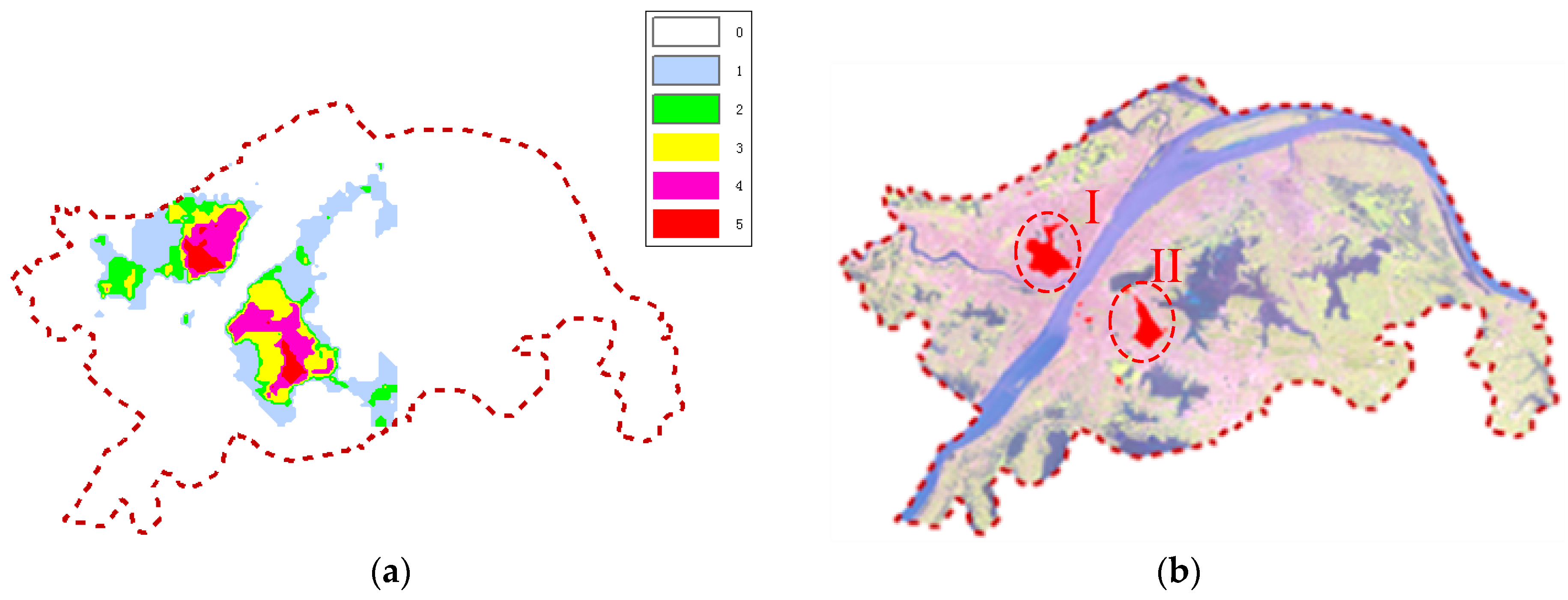
Section 3 will describe a series of experiments, including the comparison with the clustering algorithms, multi-density objects clustering and spatial analysis on Wuhan’s business circle. The subject of every experiment is different. Section 4 will conclude the paper with a summary and outlook.

2. Methods

Wu [21] proposed a global structural method to approximate aggregation characteristics of point cluster using the convex hull hierarchical structure. The global structure of geospatial points is aimed at revealing characteristics of points by ignoring individual differences. In this section, we first introduce the design thought and principle of the clustering algorithm in Section 2.1. We then propose a hierarchical clustering method based on the global structure analysis by establishing the boundary retraction structure in Section 2.2 and implement the divisive clustering of multi-density geospatial objects in Section 2.3.

2.1. Design Concept and Principle

Compared to AHC algorithms, DHC algorithms start at the top with all objects in one cluster. The cluster is split based on the global structure analysis of geospatial objects. In the process of geospatial objects clustering, the convex hull is used to describe the global structure by regarding the objects as an “organism”. Considering that spatial differentiation characteristics of the “organism” are mainly embodied between the adjacency connected clusters, the following strategies are adopted in order to explore the underlying differences of spatial clusters and split the ”organism” with an appropriate terminate condition. At first, the retracting structure of geospatial objects is built based on the convex hull borderline. Then, similar to the process of cell division, the borderline is concave so that a cluster is split into two sub-clusters when the boundaries intersect.

2.2. Boundary Retraction

Zhou [22] took the mean distance of geospatial objects as the constraint for convex hull boundary retraction. However, it is difficult to build a retracting structure of multi-density objects using invariant parameters. In this paper, the parabola-based convex hull retraction method is proposed, which is an adaptive way to obtain a cluster boundary for multi-density geospatial objects.
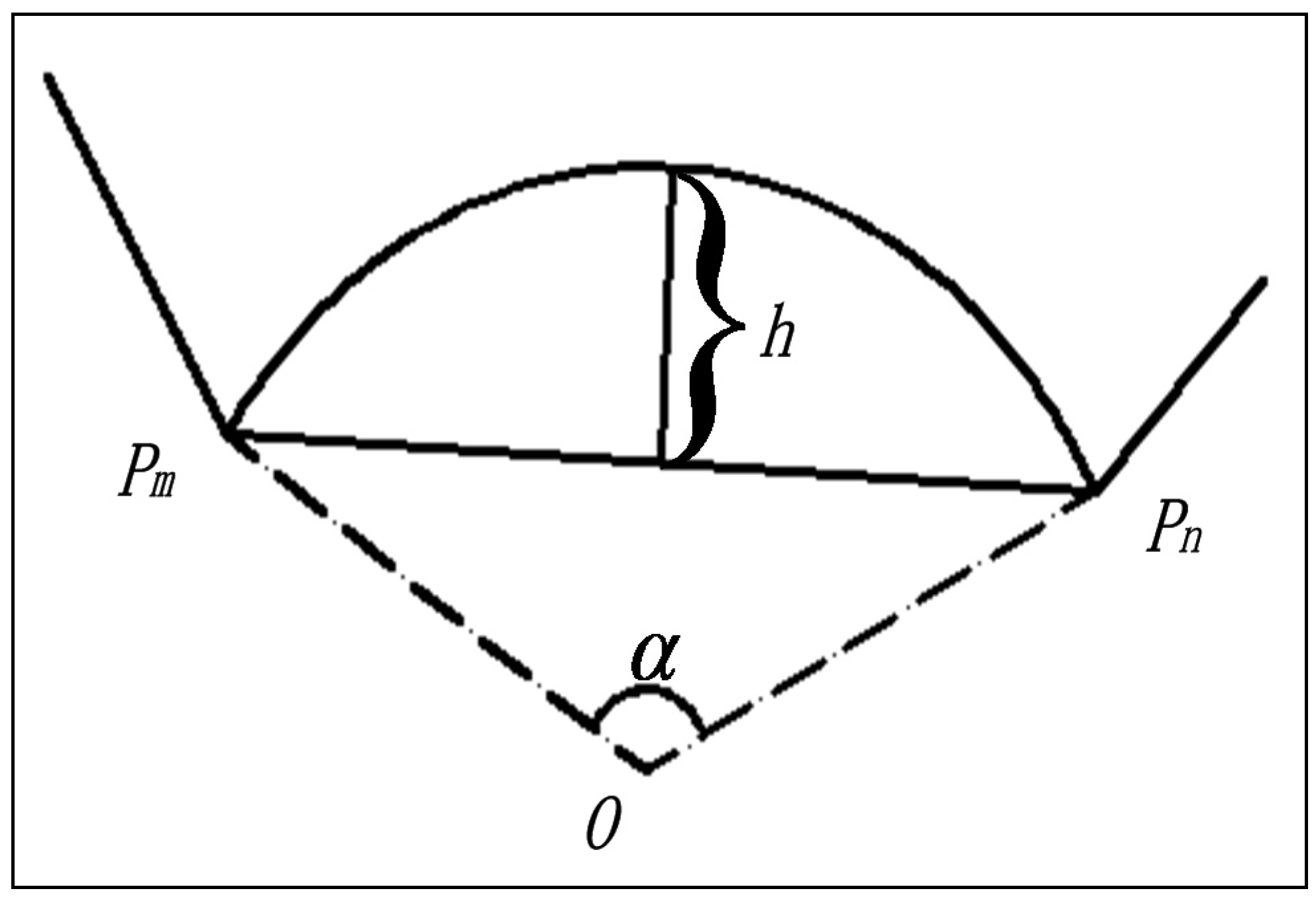
Li [23] used an arc as a boundary to generate a retraction area. The concept of retracting accuracy (RA) is introduced to limit the accuracy of a clustering boundary. Thus, the retracting accuracy of a discrete point set P is obtained as follows:
(a)
the convex hull Pc of the discrete point cluster P is constructed;
(b)
an arc with the radian of α towards the inside of the convex hull is drawn through two consecutive points Pm and Pn in the convex hull Pc (Figure 1);
(c)
the retracting accuracy α is made from the arc and line P m P n ¯ , and the retracting depth is h.
According to the arc-limited retracted method, during discrete boundary detection, the range of the retracting accuracy is in [0, π] and retracting depth is h | P m P n | 2 . The retracting depth will decrease with the length of the borderlines; therefore, using the arc-limited retracted method, it is difficult to make the borderlines intersect.
In this study, we modified the range of retracting accuracy in [0, 2π]. At the same time, we compared the arc-based method with the new parabola-based convex hull retraction method.
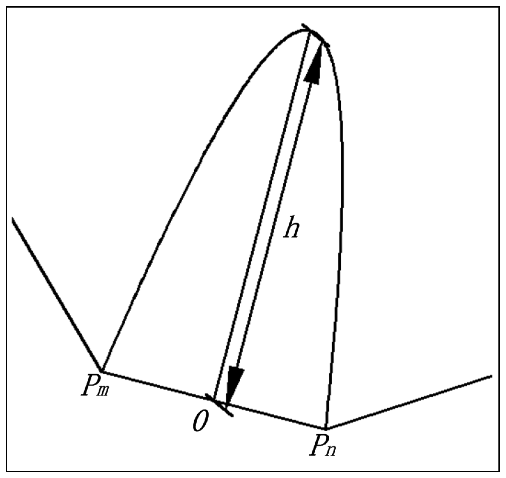
The calculation of retracting accuracy in the parabola-based convex hull retraction method is similar to the arc-based convex hull retraction method. The procedure is as follows:
(a)
construct the convex hull Pc of the discrete point cluster P;
(b)
draw a parabola towards the inside of the convex hull through two consecutive points Pm and Pn in the convex hull Pc (Figure 2). The midpoint of P m P n ¯ is the origin of the parabola, and the parabolic function complies with Equation (1);
2 ( h y ) = γ x 2 ( | x | | P m P n | 2 )
(c)
obtain the retracting accuracy made from retracted boundary P m P n ¯ and parabola P m P n , its value is γ , and the retracted depth is h.
Even with the same retracting accuracy for the boundary, the retracting area will vary because the boundary retracting depth is different. Therefore, we can adjust the retracting area according to the objects’ density around the boundary when managing multi-density discrete geospatial objects.
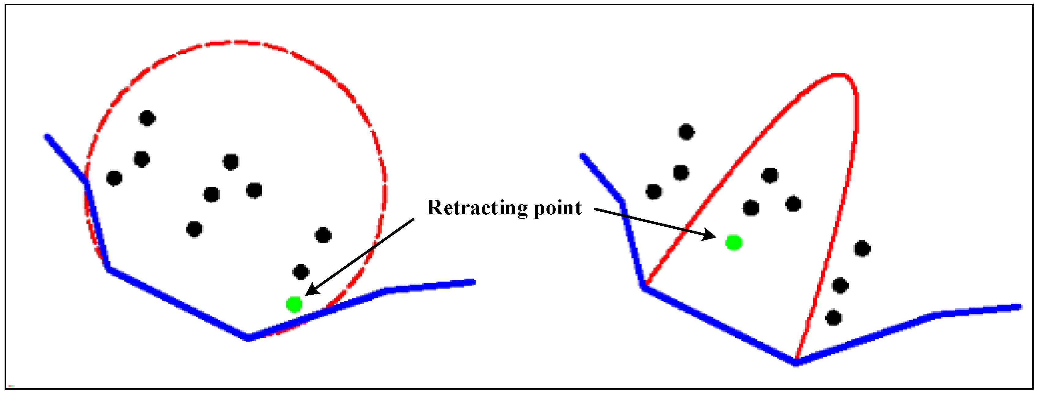
Figure 3 shows the arc and parabola retraction structure at different limiting conditions. According to the comparison, we can draw the following conclusion. With the same retracting depth, the retraction area based on arc retraction structure is larger than that based on parabola retraction structure. There are 10 points that need to be inspected in the retraction area based on arc retraction structure, but only four points need to be inspected in the retraction area based on parabola retraction structure. Therefore, the new parabola retraction structure has higher detection efficiency than that of arc retraction structure. In addition, the point chosen to retract the cluster borderline using these two methods is different. In Figure 3, the chosen point is too close to the right side around the boundary line using the arc retraction structure, and the retracted boundary will form a big twist. Compared with the arc retraction structure, the point chosen to retract the boundary in the parabola area is more reasonable.
The causes of this difference can be summarized as follows. The angle of the boundary line and the tangent of the points in the parabola is smaller than 90°, and the arc retraction structure is more divergent in the geographical space. As a result, the parabola retraction structure is used to form the retraction area and implement the clustering method.

2.3. Clustering Processing

After constructing the convex hull of geospatial points and determining the value of the retracting accuracy γ 
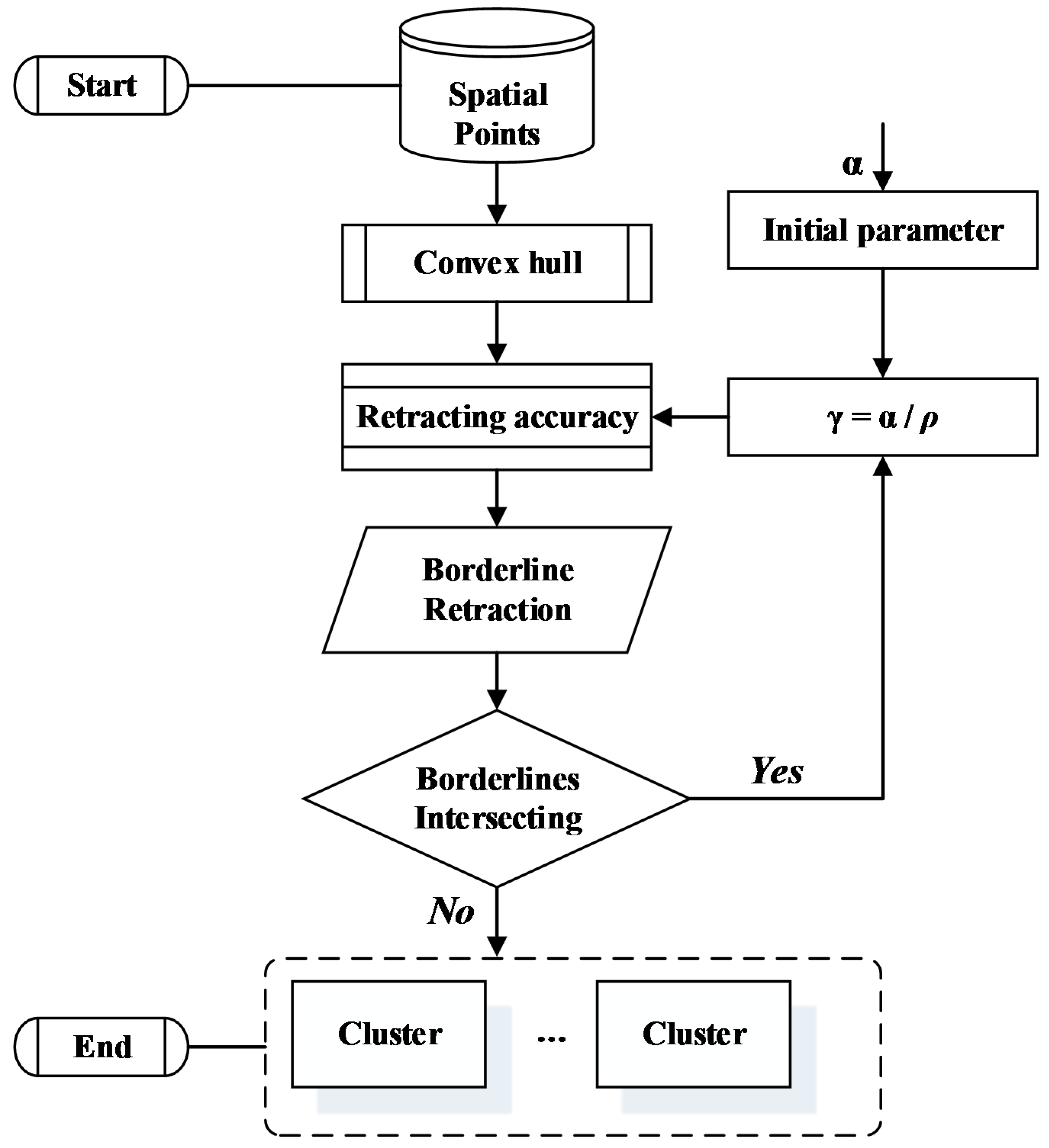
, we establish the parabola retraction area for each borderline of the convex hull. For longer borderline lengths, the cluster is easier to split between geospatial points of the borderline. It becomes possible to continuously retract the line segments where two different sub-clusters connect. The borderline retraction will not stop until the cluster is split. In Figure 4, the flow diagram displays the divisive hierarchical clustering algorithm based on convex hull retraction.
The following is the complete procedure of the algorithm:
Step 1: construct the minimum convex hull of geospatial points;
Step 2: construct the borderline retraction structure in sequence by traversing the geospatial points starting from the longest boundary line in the convex hull;
Step 3: assign the initial parameter value α.
The value of retracting accuracy γ is determined according to the point density near the convex hull borderlines. The estimation method of point density is shown as Equation (2):
ρ ¯ = S N ,
where ρ ¯ is the estimated point density in the convex hull, S is the area of the convex hull, and N is the quantity of points inside the convex hull. The calculation of boundary retracting accuracy is shown as Equation (3):
γ = α ρ ¯ ,
After setting the initial value of parameter α , it will be applied to the clustering algorithm. Each time a new sub-cluster is obtained, the convex hull area and the quantity of geospatial objects in the sub-cluster will change. The clustering process homogenizes the object distribution in geographical space and guarantees that retracting accuracy γ converges with changing ρ ¯ . The best clustering results appear when the initial value of parameter α ranges between [1,2] based on a large number of experiments.
Step 4: retracting borderlines
There are two purposes for constructing the parabola retracting structure. One is to limit the search area to improve efficiency, and the other is to define it as a termination condition of the split clustering. We construct the retraction structure in sequence according to the length of the convex hull borderlines. The procedure is shown in 
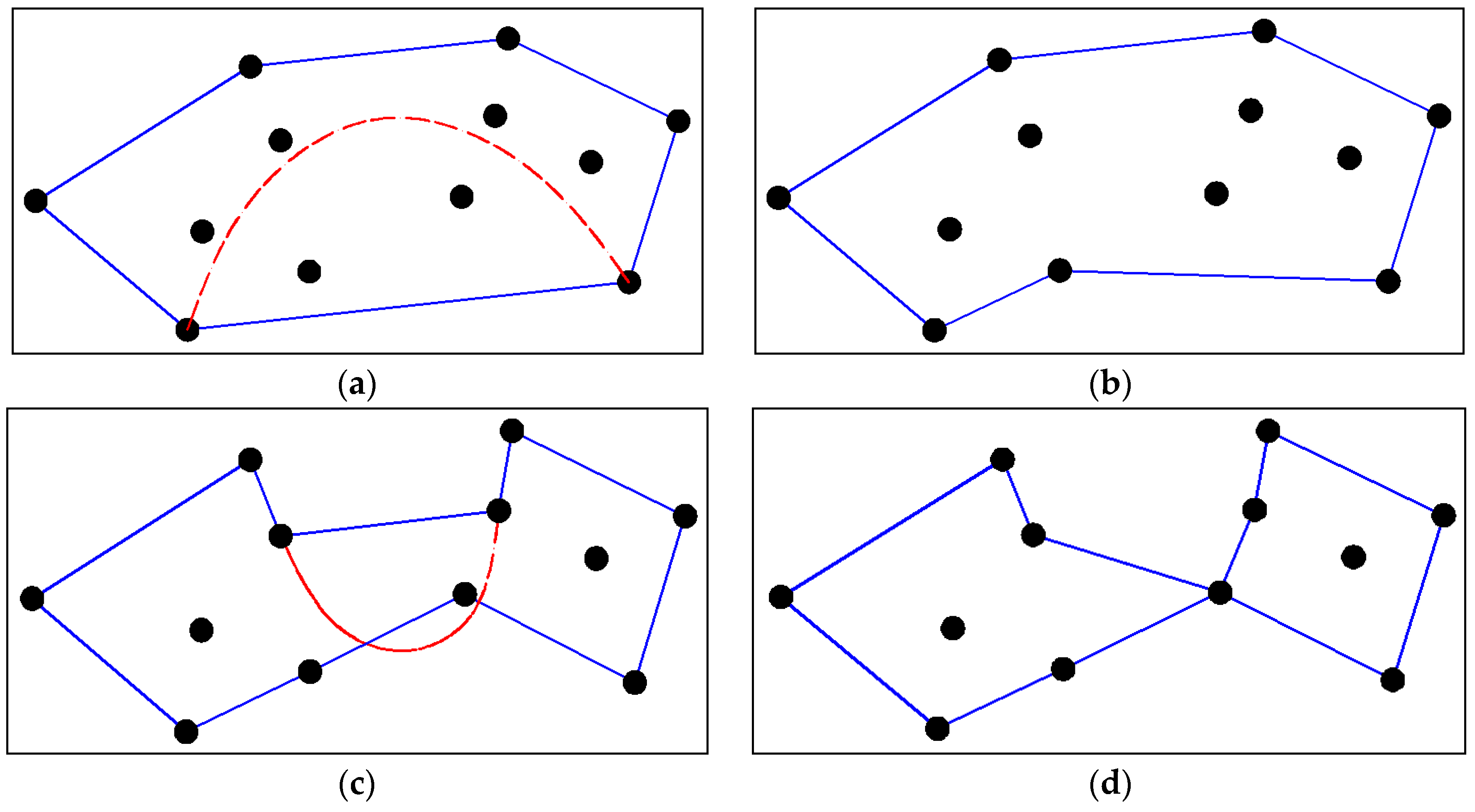
Figure 5. First, we construct the retracted structure of the longest borderline of the convex hull. Second, we find all points inside the retracting area and set the point, which is closest to the borderline as the retracting point. If objects in the area are empty, the borderline is marked as “0”. Figure 5 shows a complete process of borderline retracting and the cluster division. If the nearest point inside the retracting area belongs to the borderline point, as shown in Figure 5c, the cluster will be divided into two sub-clusters. Figure 5d shows the result of division. We can find that two sub-clusters share a common point after dividing. We can determine which sub-cluster the common point belongs to based on the distance from the point to the nearest point of the sub-cluster.
Step 5: sub-cluster partitions
The sub-cluster obtained by the points division can be regarded as an independent cluster. Then, we repeat Steps 2 to 4 until all the borderlines of the sub-clusters are marked as “0”. If there are no more than three points in a sub-cluster and it is not able to build a convex hull, the points are regarded as noise.
The clustering process above is similar to the process of cell division in biology. Therefore, we name the clustering algorithm Cell-dividing Hierarchical Clustering (CDHC for short).

3. Experiments and Results

A series of experiments are conducted to validate the efficiency of the CDHC algorithm in comparison to the traditional AHC algorithm and the Delaunay triangulation clustering algorithm. We also verify the superiority of the CDHC algorithm in dealing with the multi-density objects.

3.1. Experiment 1—Comparison of Clustering Algorithms

The experiment is designed to test the effectiveness through comparison of different calculation results. A set of points with edge noises, as shown in Figure 6a, are chosen as the experimental data. It is clear that there are two point clusters, which are surrounded by noisy points. The CDHC algorithm is used to cluster the experimental data with the initial parameter of α = 1.45 and the clustering result is shown in Figure 6b.
The traditional AHC algorithm takes each object as an independent class. For a given set of N objects (N = 0, 1, 2, …, n), there are N classes and each class contains one object at the beginning. Therefore, an N × N distance matrix can be obtained. The distance between two classes is computed as the distance between objects in the two classes. The nearest two classes are merged, and the distance between the new class and the original classes are recalculated. The remainder is done in the same manner until all the classes are merged into a class or the distance between two classes reaches a given threshold. Figure 6c shows the clustering result using the traditional AHC algorithm with 5.0 as the threshold.
Li [24] proposed the clustering algorithm based on Delaunay triangulation (CBDT). The clustering of the experimental data using the CBDT algorithm is accomplished in three steps. First, the Delaunay triangulation is constructed for the point set. Second, all triangles are classified into three categories, i.e., small triangles, long–narrow triangles and big triangles, according to the ratio of the triangle area to the side length. Finally, the clustering result is generated by deleting long–narrow triangles and big triangles. Figure 6d shows the Delaunay triangulation of the experimental data. Figure 6e shows the clustering result using the CBDT algorithm with K = 2.5 (K is the ratio of the longest side to the shortest side of the triangle).
Through a comparison of clustering results using the CDHC algorithm, the CBDT algorithm and the traditional AHC algorithm, it can be inferred that the CDHC algorithm can handle the clustering analysis of spatial data well and is capable of resisting noise.
To compute an N × N distance matrix, the time complexity using the AHC algorithm is O(n2), and the time complexity using the CDHC algorithm is O(Kn), where K is the number of clusters and K < n. A personal computer with a Windows 32-bit operating system, 2.6 GHz processor and 1G physical RAM serves as the experimental platform. The comparative result of time complexity between CDHC and AHC algorithms is shown in Table 1.
According to Table 1, the CDHC algorithm is superior to the traditional AHC algorithm in dealing with a large number of geospatial points. However, the noise points are processed as a cluster when the CDHC algorithm is adopted. Thus, the efficiency of the CDHC algorithm is lowered due to the noise points.
The spatial clustering using the CBDT algorithm is based on the identification of the triangle shape after Delaunay triangulation. The clustering result is sensitive to the noise points between two sub-clusters. In addition, an improper K will lead to a combination of two sub-clusters or separation of a sub-cluster. To avoid the merging of two sub-clusters, a small K is used in Figure 6e. It appears that some points in the same sub-cluster are classified as noise.

3.2. Experiment 2—Clustering of Multi-Density Objects

The objective of this experiment is to highlight advantages of the proposed CDHC algorithm. The first sets of data, multi-density points without noise, are clustered using the CDHC algorithm, and two additional sets of data with noise are processed using different clustering methods in the following manner.
We manage multi-density objects with noises using the CDHC algorithm in experiment 2. The first experimental data are multi-density objects without noise, as shown in Figure 7a, and there are three geospatial point sets with different densities. The CDHC algorithm is used to process the multi-density points with the initial parameter of α = 1.75. The clustering result is shown in Figure 7b.
As shown, the CDHC algorithm identifies multi-density objects well. To clarify this point further, two other experiments are carried out using CDHC algorithm, while the CBDT algorithm, DBSCAN algorithm and another common clustering algorithm, K-means, were taken as comparisons. For multi-density objects and noise, these algorithms share many characteristics; therefore, the two experiments are to test sufficient separation of the multi-density objects from noise. There are two clusters in one of the experimental data with abundant noise in Figure 8a, and the other experimental data are multi-density objects with a little noise, as shown in Figure 9a. The cluster analysis has been applied to the experimental data using CDHC, CBDT, DBSCAN and K-means algorithms.
Through a comparison of clustering results, CDHC, CBDT and DBSCAN algorithms can resist noise while managing general experimental data in spite of the noise. The three methods have the advantage of good anti-noise ability with a recognition rate of 95% in Figure 8b–d. However, the traditional clustering method, K-means algorithm, does not have the ability to identify effective data and noise, as shown in Figure 8e. Then, the three algorithms are applied to multi-density objects with a little noise. The results show that the three clusters with different-density objects can be identified from the noise in Figure 9b. The CDHC algorithm adopts the variable of retracting accuracy and enjoys a strong advantage in dealing with multi-density geospatial points. However, it is difficult to apply the CBDT algorithm to cluster the multi-density points based on the triangle shape in Figure 9c, and the recognition rate is reduced up to 70%, that is, because the method does well in identifying the internal structure of clusters through triangle subdivision and ignores the global spatial context of geospatial objects. Compared with the clustering result using the CDHC algorithm, we find that one noise point in the dashed circle is not identified correctly using DBSCAN algorithm in Figure 9d. DBSCAN can find non-linearly separable clusters and even more complex shapes, but it cannot cluster data sets well with large differences in densities. If the distance between the points of the right cluster is enlarged, we will not obtain satisfactory results such as the clustering result above. The K-means algorithm is a general clustering method to find cluster centres that minimize intra-class variance. Although the cluster centres can be accurately identified, the geospatial objects with multi-density are challenging, and partitioned into the wrong cluster. As is shown in Figure 9e, the clustering result is far from the expected goal.

3.3. Experiment 3—Application of CDHC Algorithm for Spatial Analysis

This experiment is aimed at performing the spatial analysis of retail agglomeration in business circles in Wuhan, China, using the CDHC algorithm. The main function of a business circle is to convince customers to make purchases. Whatever the business circle orientation, the food service industry can generally represent the commercial prosperity in Chinese cities and towns. Hence, the restaurants in Wuhan’s Central District are chosen as the experimental data (as shown in Figure 10), which are divided into five types: Chinese restaurant, Western restaurant, hot-pot restaurant, fast food and supermarket. The spatial distribution of these restaurants reflects a wide variety of consumption activities.
Located at the intersection of the middle reaches of the Yangtze River and the Han River, Wuhan is divided into three districts, i.e., Wuchang, Hankou and Hanyang, and sprinkled with many lakes in the central district. It can be observed that many restaurants are divided or gathered by the natural topographic conditions and water systems. At first, the spatial clustering analysis of the five types of restaurants is performed using the CDHC algorithm. Then, the clustering result is subject to the overlay analysis, which gives rise to a thematic map shown in Figure 11a.
In the map, 0 to 5 represent the number of overlaying layers, respectively. For example, the regions where the number of overlaying layers is 5 are displayed on the satellite image of Wuhan in Figure 11b. By referring to the map, there are two main regions: the left region (I) is near the Yangtze River and Han River in Hankou, and the right one (II) is located at the centre of Wuchang. The results are compared with the planning and development of the business circles. We find that the WuGuang and Jianghan Road business circles are located in region I, and region II contains the Xudong, Zhongnan and Jiedaokou business circles. The two regions are within the most economically developed areas in Wuhan, and the results of this experiment match well with the current commercial development situation in Wuhan.

4. Discussion and Conclusions

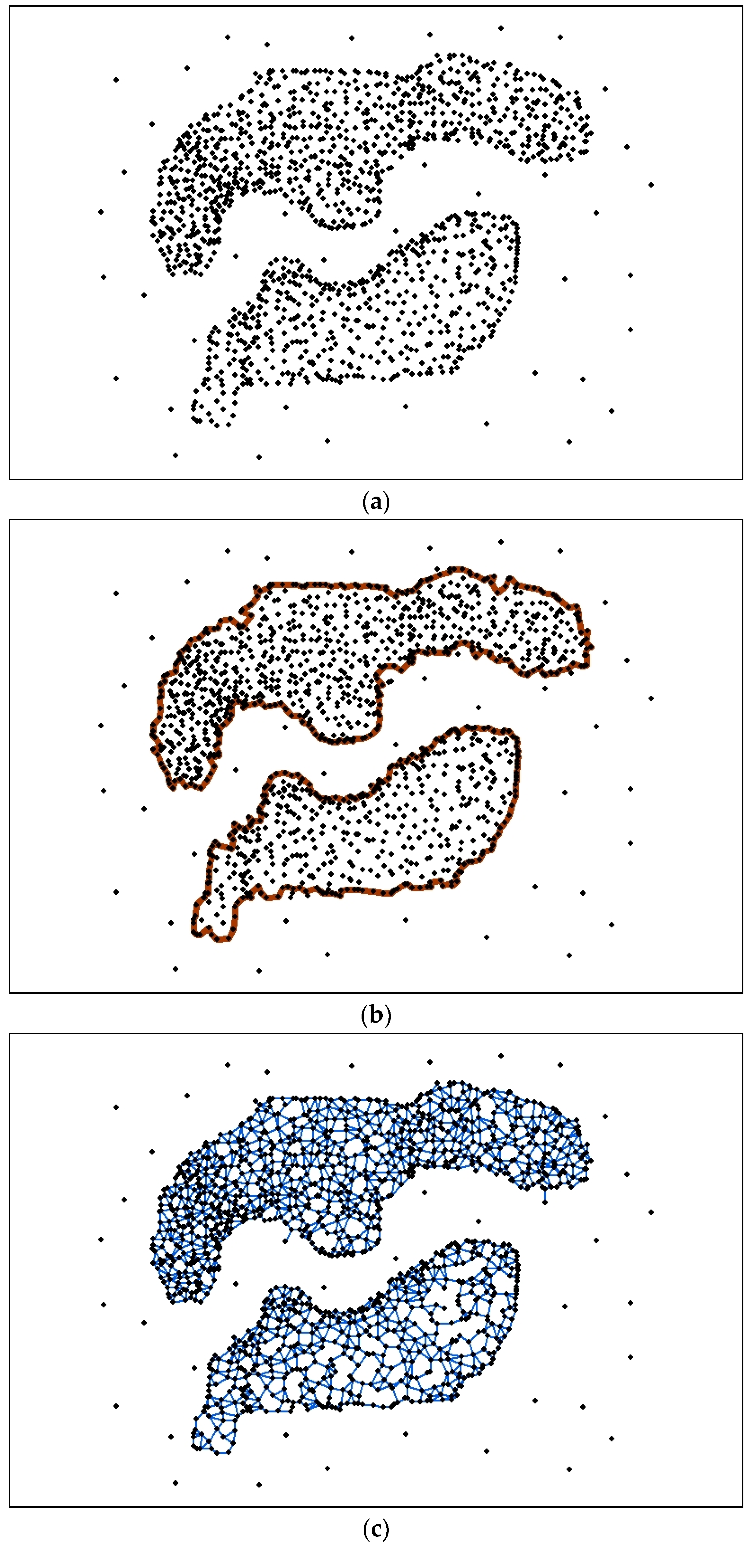
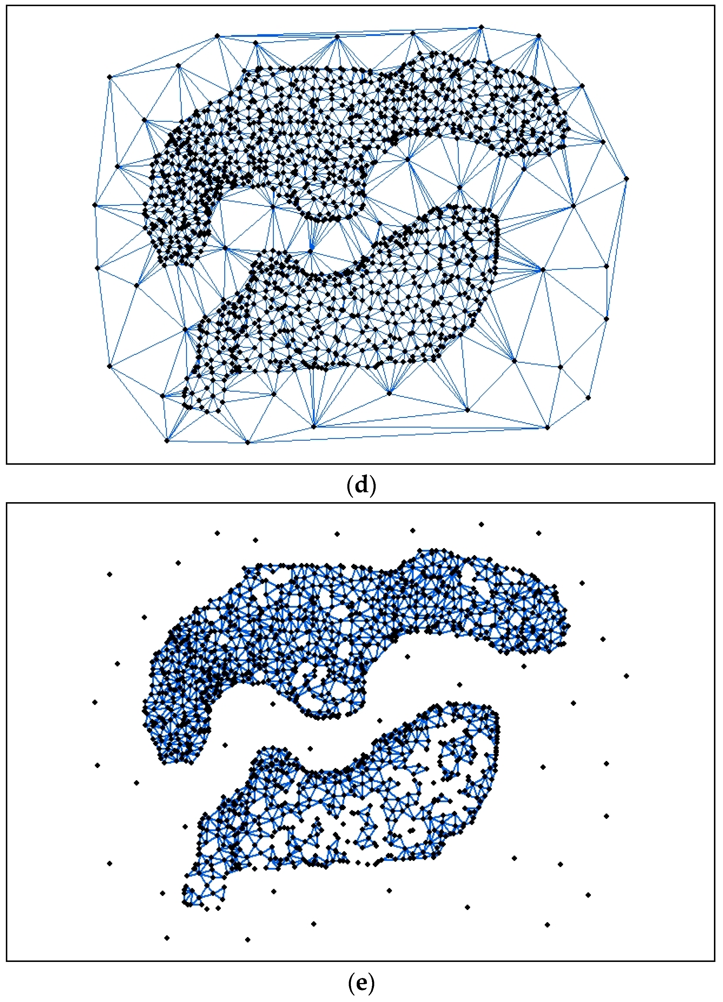
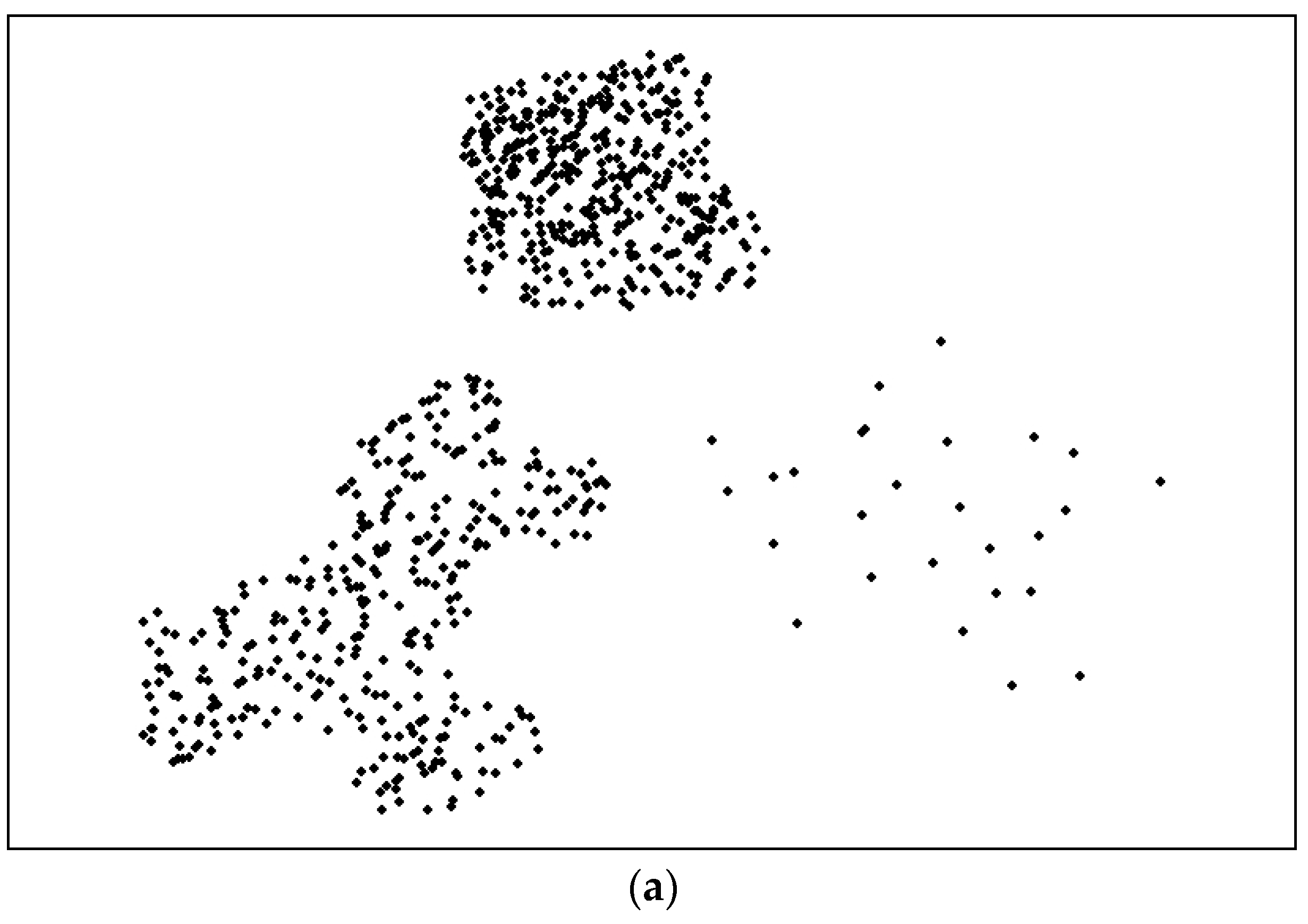
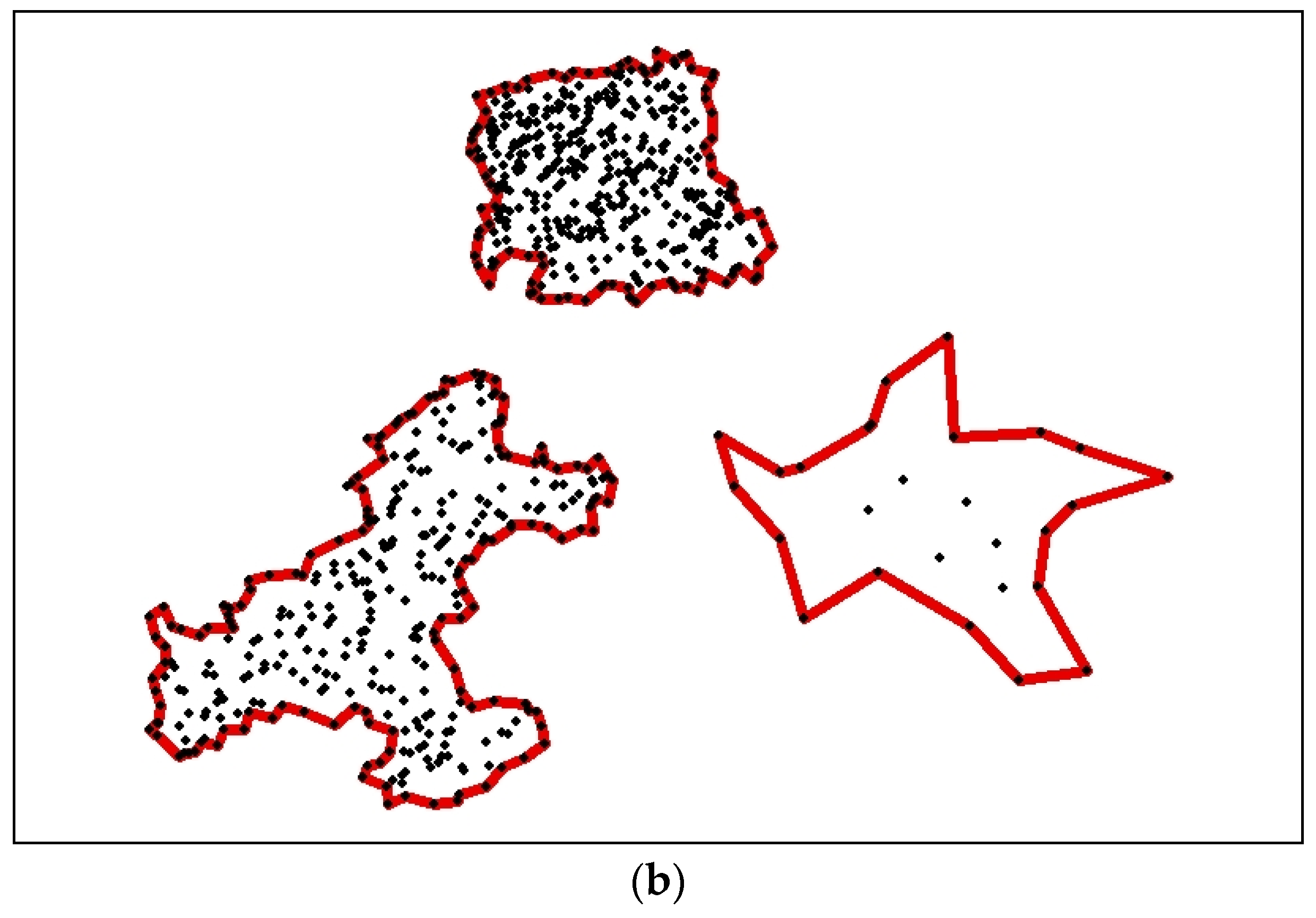
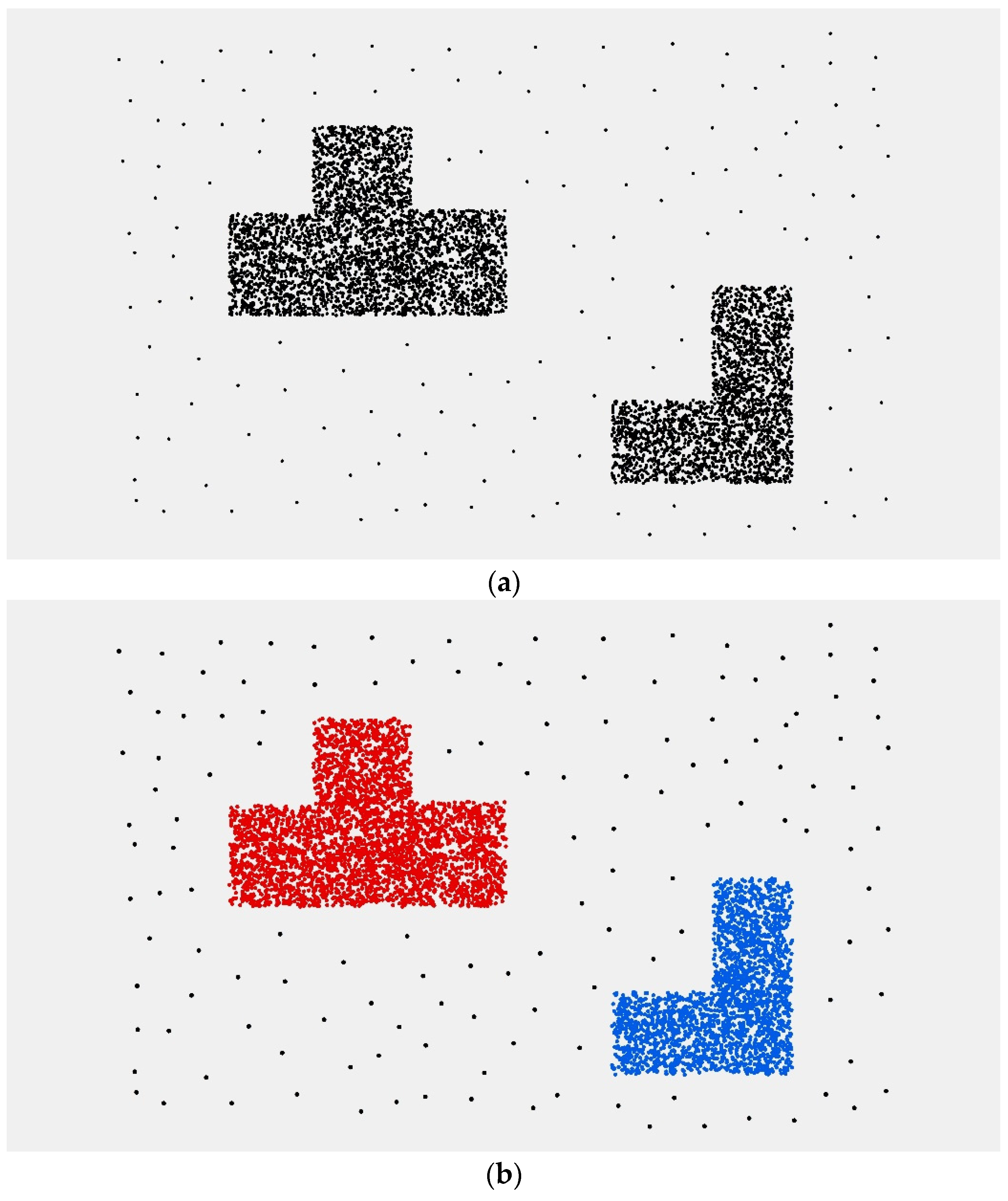
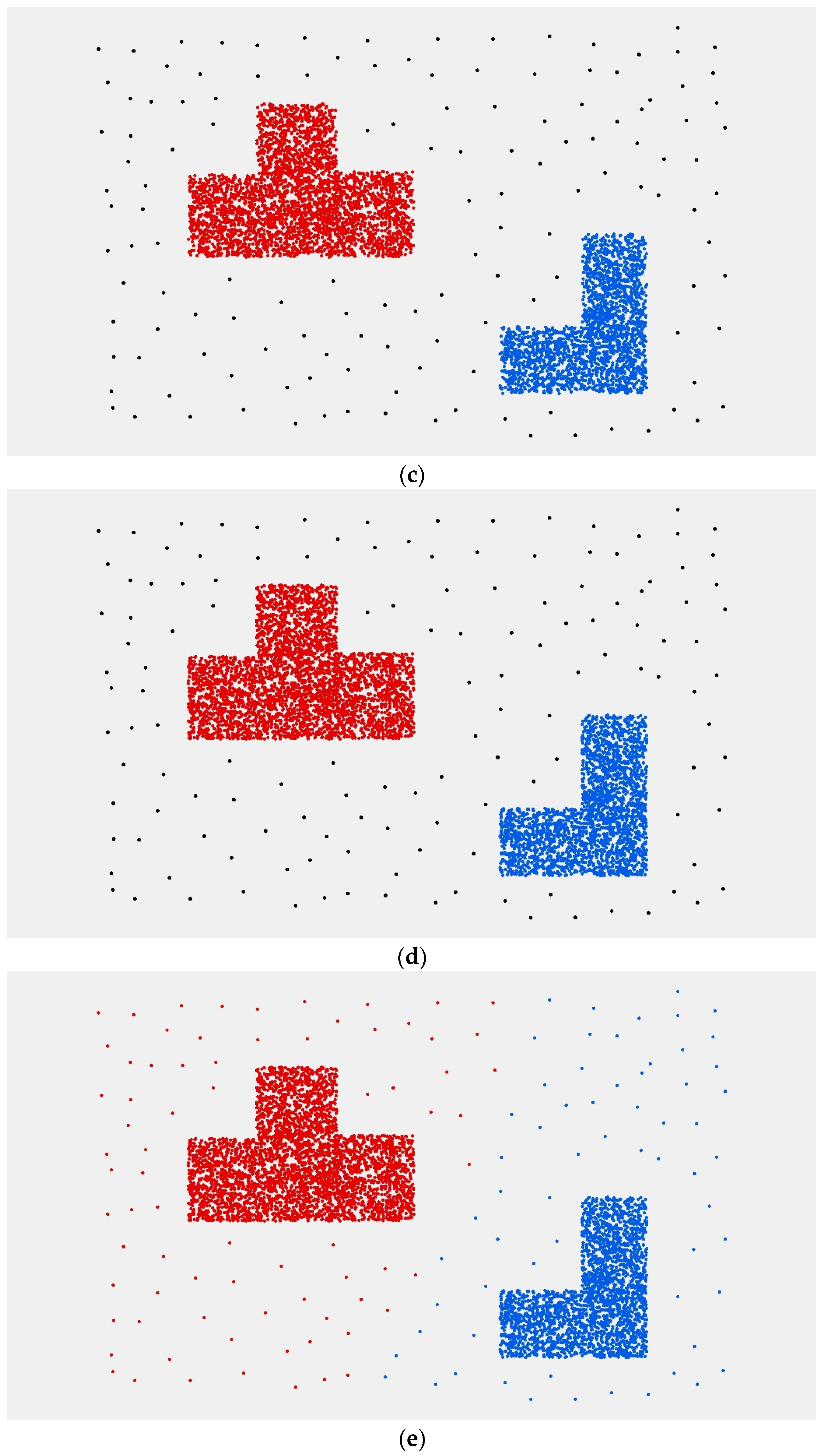
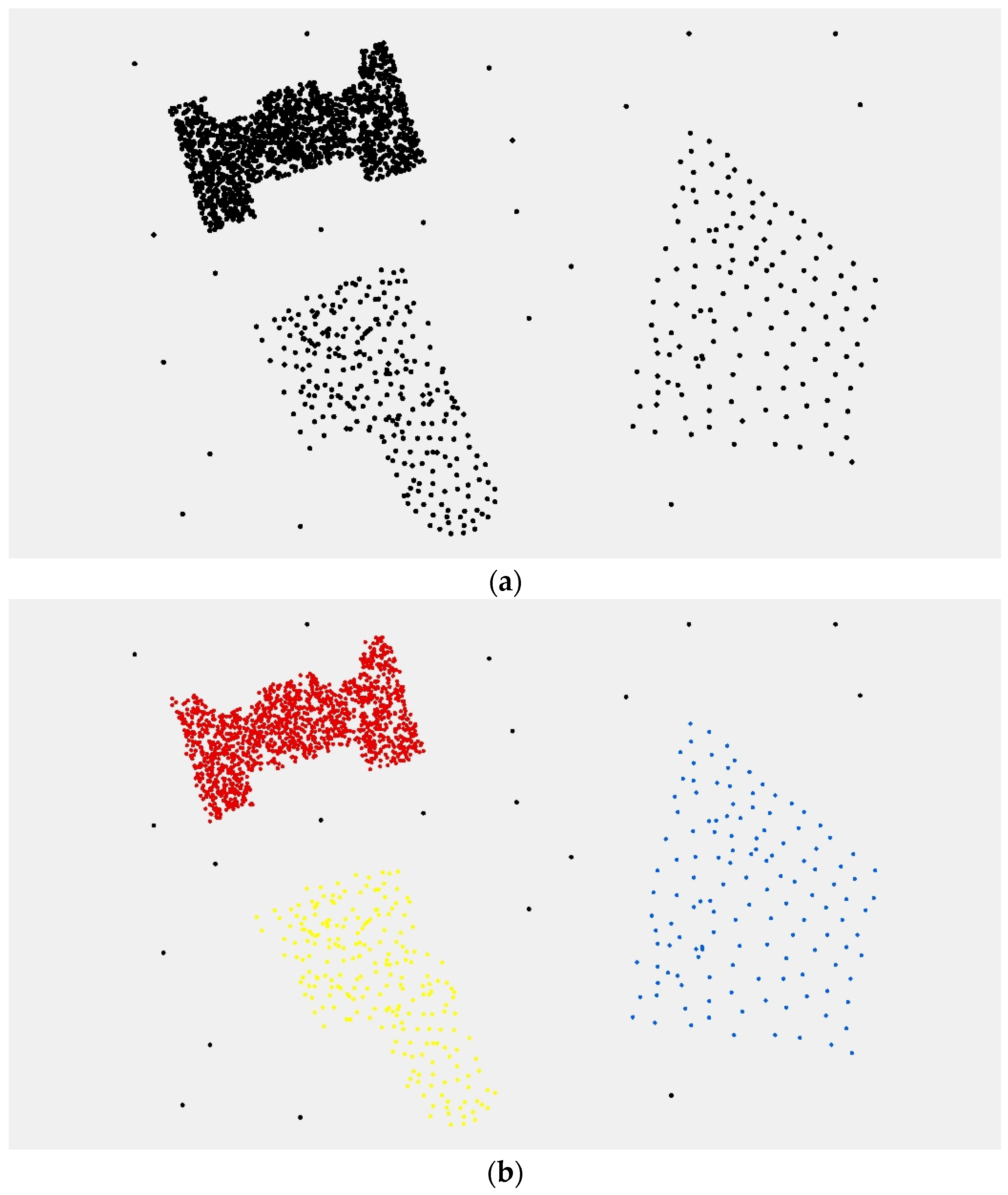
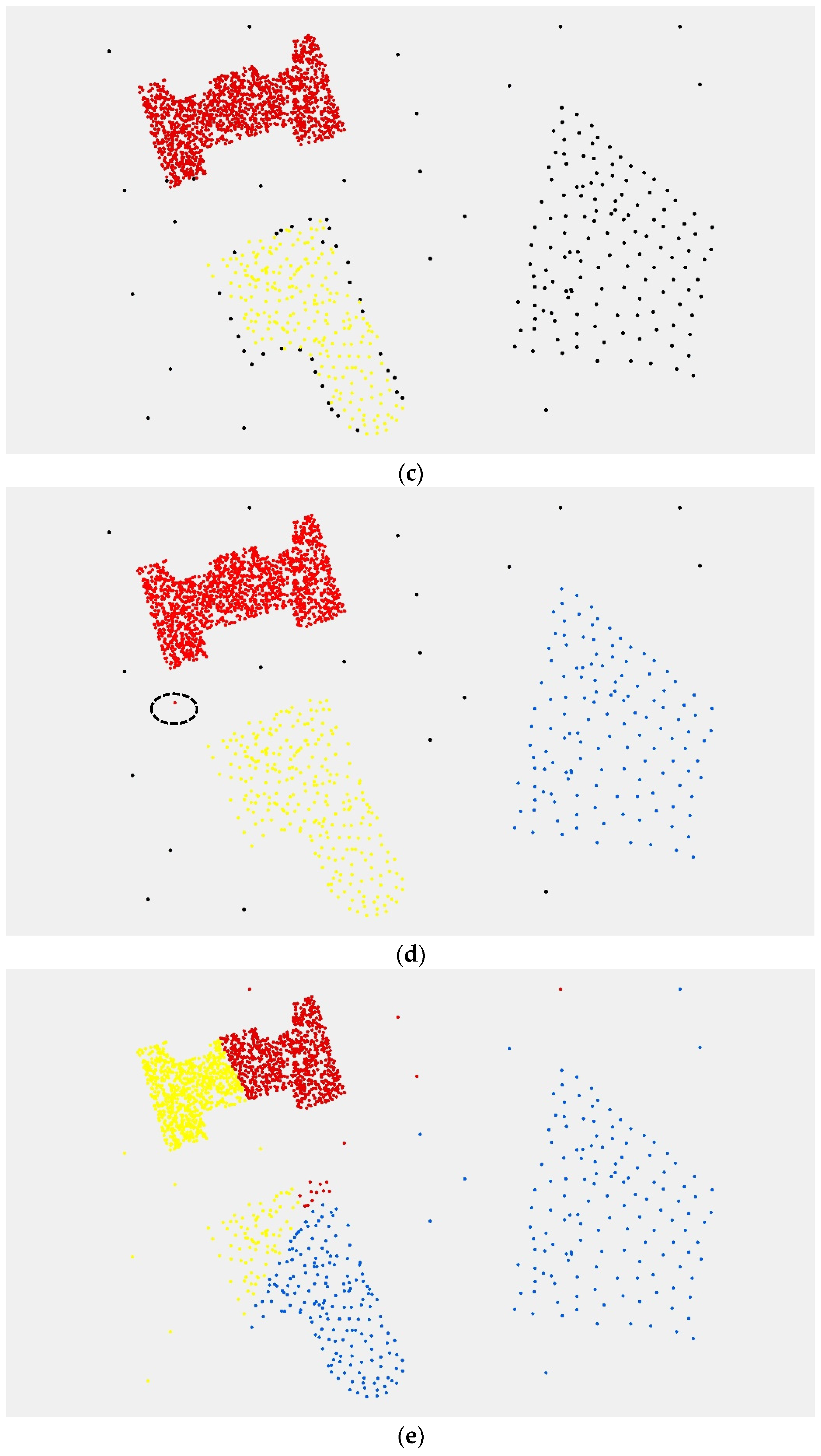
Spatial clustering algorithms are developed to group a set of objects in such a way that discrete objects in the same group, which are close to each other, are separate from those in other groups. However, there is a similarity of spatial structure between multi-density objects and noise data. Thus, it becomes more difficult to distinguish between the two in the local spatial context. It is necessary to address multi-density discrete objects based on a global spatial structure. In this paper, a modified convex hull structure is presented to describe the global spatial context of discrete objects. A boundary retraction is used to mine spatially stratified heterogeneity between clusters in our clustering method. Then, the boundary structure of each sub-cluster describes the global spatial context of the new subset. The density of spatial objects is used as the termination condition of the algorithm, so the CDHC algorithm can easily distinguish noise from multi-density objects.
Algorithmic efficiency has long been one of the issues in clustering analysis when dealing with large amounts of data. Many clustering algorithms work well in processing a small amount of data, but algorithm performance becomes worse as the data volumes grow. After comparison with two hierarchical clustering algorithms in experiment 1, we find that the CDHC algorithm has advantages in dealing with a large amount of spatial objects. The CDHC algorithm is a divisive hierarchical clustering, applying a “top–down” approach: all spatial objects start in one cluster and are split into two sub-clusters by the hierarchy. This avoids computing the position of each object at each iteration, so the CDHC algorithm can significantly improve efficiency of clustering analysis.
This paper proposes a new spatial clustering algorithm: cell-dividing hierarchical clustering (CDHC), which manages multi-density geospatial points. The CDHC algorithm can describe the global spatial context of geospatial points by establishing a minimum convex hull structure. After a cluster is split into two sub-clusters due to boundary retraction, each sub-cluster will be split again in the same way. Thus, it can be seen that geospatial points can be classified based on global structure at all times. Then, the algorithm uses a parabolic-limited retracted method to split the points, and achieve the requirements of split hierarchical clustering.
The experimental results show that the noise points and multi-density point sets are well identified using the CDHC algorithm. In addition, the CDHC algorithm can extract the internal differentiation regularity of a geospatial objects cluster using a variable parameter strategy according to the characteristics of spatial clusters. The CDHC algorithm avoids the uncertainty resulting from deterministic parameters, as well as the high computational complexity required by traditional hierarchical clustering algorithms. Although the CDHC algorithm has the ability to identify the points at boundaries, it is unable to address the clusters contained within another cluster. The improved DBSCAN methods are able to handle this challenge, although there are still some problems and limitations. Future work will continue research in this area, combining the two clustering methods to solve the multi-density clustering problem.

Acknowledgments

This work was supported by the Chinese Natural Science Foundation Project (41271449).

Author Contributions

Shaoning Li conceived the study topic and the clustering algorithm; Wenjing Li selected the study areas and processed the data; Jia Qiu analyzed the results; and Shaoning Li wrote the paper.

Conflicts of Interest

The authors declare no conflict of interest.

Abbreviations

The following abbreviations are used in this manuscript:
RA
Retracting Accuracy
AHC
Agglomerative Hierarchical Clustering
DHC
Divisive Hierarchical Clustering
CDHC
Cell-dividing Hierarchical Clustering
CBDT
Clustering algorithm based on Delaunay Triangulation
DBSCAN
Density-Based Spatial Clustering of Applications with Noise

References

  1. Kreis, C.; Grotzer, M.; Hengartner, H.; Daniel, S.B. Space-time clustering of childhood cancers in Switzerland: A nationwide study. Int. J. Cancer 2016, 138, 2127–2135. [Google Scholar] [CrossRef] [PubMed]
  2. Ghaffarian, S.; Ghaffarian, S. Automatic histogram-based fuzzy C-means clustering for remote sensing imagery. ISPRS J. Photogramm. Remote Sens. 2014, 97, 46–57. [Google Scholar] [CrossRef]
  3. Zheng, N.; Zhang, H.; Fan, J.; Guan, H. A fuzzy local neighbourhood-attraction-based information c-means clustering algorithm for very high spatial resolution imagery classification. Remote Sens. Lett. 2014, 5, 843–852. [Google Scholar] [CrossRef]
  4. Ai, T.; Guo, R. Polygon cluster pattern mining based on gestalt principles. Acta Geod. Cartogr. Sin. 2007, 36, 302–308. [Google Scholar]
  5. Mao, Z. The study of extracting structure information of a clustered spatial point pattern. Acta Geod. Cartogr. Sin. 2007, 36, 181–186. [Google Scholar]
  6. Jia, S.; Tang, G.; Zhu, J.; Li, Q. A novel ranking-based clustering approach for hyperspectral band selection. IEEE Trans. Geosci. Remote Sens. 2016, 54, 88–102. [Google Scholar] [CrossRef]
  7. Sun, X.; Yang, L.; Gao, L.; Zhang, B.; Li, S.; Li, J. Hyperspectral image clustering method based on artificial bee colony algorithm and Markov random fields. J. Appl. Remote Sens. 2015, 9, 1–19. [Google Scholar] [CrossRef]
  8. Ma, A.; Zhong, Y.; Zhang, L. Spectral-spatial clustering with a local weight parameter determination method for remote sensing imagery. Remote Sens. 2016, 8, 124. [Google Scholar] [CrossRef]
  9. Ameri, F.; Mohammad, J. Road vectorisation from high-resolution imagery based on dynamic clustering using particle swarm optimisation. The Photogramm. Rec. 2015, 30, 363–386. [Google Scholar] [CrossRef]
  10. Guo, Q.; Zheng, C.; Hu, H. Hierarchical clustering method of group of points based on the neighborhood graph. Acta Geod. Cartogr. Sin. 2008, 37, 256–261. [Google Scholar]
  11. Chacon-Murguia, M.I.; Ramirez-Quintana, J.; Urias-Zavala, D. Segmentation of video background regions based on a DTCNN-clustering approach. Signal Image Video Process. 2015, 9, 135–144. [Google Scholar] [CrossRef]
  12. Wikipedia. Clustering Analysis. Available online: https://en.wikipedia.org/wiki/Cluster_analysis (accessed on 1 May 2016).
  13. Sun, J.; Liu, J.; Zhao, L. Clustering algorithms research. Chin. J. Softw. 2008, 19, 48–61. [Google Scholar] [CrossRef]
  14. Zhou, X.; Yao, P.; Xin, W. Command and control resource deployment based on improved hierarchical clustering method. J. Syst. Eng. Electron. 2012, 34, 523–528. [Google Scholar]
  15. Gelbard, R.; Goldman, O.; Spiegler, I. Investigating diversity of clustering methods: An empirical comparison. Data Knowl. Eng. 2007, 63, 155–166. [Google Scholar] [CrossRef]
  16. Chen, Y. Research of spatial clustering of discrete points in direction. Comput. Eng. Appl. 2012, 48, 7–10. [Google Scholar]
  17. Pradeep, L.; Sowjanya, A.M. Multi-density based incremental clustering. Int. J. Comput. Appl. 2015, 116, 6–9. [Google Scholar] [CrossRef]
  18. Mitra, S.; Nandy, J. KDDClus: A Simple Method for Multi-Density Clustering. In Proceedings of International Workshop on Soft Computing Applications and Knowledge Discovery (SCAKD 2011), Moscow, Russia, 25 June 2011; pp. 72–76.
  19. Gold, C. Spatial Embedding and Spatial Context. In Quality of Context; Springer: Stuttgart, Germany, 2009; pp. 53–64. [Google Scholar]
  20. Marques de Sá, J.P. Data Clustering. In Pattern Recognition Concepts, Methods and Applications; Springer: Berlin/Heidelberg, Germany, 2001; pp. 53–78. [Google Scholar]
  21. Wu, H. Principle of convex hull and its applications in generalization of grouped point objects. Eng. Surv. Mapp. 1997, 1, 1–6. [Google Scholar]
  22. Zhou, Q.; Wang, Y.; Ma, J. Research on border generation algorithm for TIN model. Bull. Surv. Mapp. 2005, 5, 30–32. [Google Scholar]
  23. Li, W.; Li, S.; Qiu, J.; Zhou, T. Boundary detection of multi-density point cluster using convex hull retracted method. Sci. Surv. Mapp. 2014, 39, 126–129. [Google Scholar]
  24. Li, J.; Chen, L.; Cheng, H.; Nie, Y. Study of spatial clustering algorithm based on delaunay triangulation. Comput. Technol. Dev. 2009, 19, 21–24, 28. (In Chinese) [Google Scholar]
Figure 1. Arc-limited retracted structure with retracting accuracy α, with P m P n ¯ as one of the convex hull borderlines, O is the centre and h is the retracting depth.
Ijgi 06 00030 g001
Figure 2. Parabola-limited retracted structure where the retracted boundary P m P n ¯ is one of the convex hull borderlines, and h is the retracting depth.
Ijgi 06 00030 g002
Figure 3. The same retracting depth at a different limiting condition.
Ijgi 06 00030 g003
Figure 4. Procedure of divisive hierarchical clustering algorithm based on convex hull retraction.
Ijgi 06 00030 g004
Figure 5. Sketch maps of retracting borderlines. (a) The parabola retraction structure; (b) Borderlines retracting for the first time; (c) Intersecting borderlines; (d) Cluster division.
Ijgi 06 00030 g005
Figure 6. Experimental results. (a) Experimental data; (b) Clustering result using the cell-dividing hierarchical clustering (CDHC) algorithm; (c) Clustering result using the traditional agglomerative hierarchical clustering (AHC) algorithm; (d) Delaunay triangulation of the experimental data; (e) Clustering result using the clustering algorithm based on Delaunay triangulation (CBDT).
Ijgi 06 00030 g006aIjgi 06 00030 g006b
Figure 7. Experimental results. (a) Experimental data; (b) Clustering result using the CDHC algorithm.
Ijgi 06 00030 g007aIjgi 06 00030 g007b
Figure 8. Experimental results. (a) Experimental data; (b) Clustering result using the CDHC algorithm; (c) Clustering result using the CBDT algorithm; (d) Clustering result using the DBSCAN algorithm; (e) Clustering result using the K-means algorithm; (f) Legend.
Ijgi 06 00030 g008aIjgi 06 00030 g008bIjgi 06 00030 g008c
Figure 9. Experimental results. (a) Experimental data; (b) Clustering result using the CDHC algorithm; (c) Clustering result using the CBDT algorithm; (d) Clustering result using the DBSCAN algorithm; (e) Clustering result using the K-means algorithm; (f) Legend.
Ijgi 06 00030 g009aIjgi 06 00030 g009bIjgi 06 00030 g009c
Figure 10. Spatial distribution of restaurants in Wuhan. (a) Wuhan’s Central District; (b) Chinese restaurant; (c) Western restaurant; (d) Fast food; (e) Hot-pot restaurant; (f) Supermarket.
Ijgi 06 00030 g010
Figure 11. Clustering results of restaurants and their locations in Wuhan’s Central District. (a) Thematic map by the overlay analysis; (b) Regions with the largest overlaying layers in Wuhan.
Ijgi 06 00030 g011
Table 1. A comparison of time complexity between CDHC and AHC algorithms.
Time(s)AlgorithmsCDHC AlgorithmAHC Algorithm
Number of Points
3551.451.24
7732.2516.11
11989.2755.75
143229.5221.01
208960.44397.27
11,5503.61 × 1034.07 × 104

