The Local Colocation Patterns of Crime and Land-Use Features in Wuhan, China


1
State Key Laboratory of Information Engineering in Surveying, Mapping and Remote Sensing, Wuhan University, Wuhan 430079, China
2
Collaborative Innovation Center of Geospatial Technology, Wuhan 430079, China
3
Department of Geography, Kent State University, Kent, OH 44242-0001, USA
4
Key Laboratory of Police Geographic Information Technology, Ministry of Public Security, Changzhou 213022, China
*
Author to whom correspondence should be addressed.
ISPRS Int. J. Geo-Inf. 2017, 6(10), 307; https://0-doi-org.brum.beds.ac.uk/10.3390/ijgi6100307
Submission received: 22 August 2017
/
Revised: 25 September 2017
/
Accepted: 16 October 2017
/
Published: 17 October 2017
(This article belongs to the Special Issue Place-Based Research in GIScience and Geoinformatics)
Abstract
:Most studies of spatial colocation patterns of crime and land-use features in geographical information science and environmental criminology employ global measures, potentially obscuring spatial inhomogeneity. This study investigated the relationships of three types of crime with 22 types of land-use in Wuhan, China. First, global colocation patterns were examined. Then, local colocation patterns were examined based on the recently-proposed local colocation quotient, followed by a detailed comparison of the results. Different types of crimes were encouraged or discouraged by different types of land-use features with varying intensity, and the local colocation patterns demonstrated spatial inhomogeneity.
1. Introduction
Quantifying the spatial relationships between geographical entities and their neighbors is a common spatial analytical topic. Tobler’s First Law of Geography states that ‘all attribute values on a geographic surface are related to each other, but closer values are more strongly related than are more distant ones’ [1]. This famous law stresses the spatial proximity of objects. Bivariate spatial association analysis, also referred to as colocation pattern mining, assesses the spatial proximity of two distinct categories [2], and is an important spatial analytical task [3].
Studies in numerous fields have demonstrated that colocation patterns exist. Arbia et al. [4] analyzed the spatial distribution of industries and found that co-agglomeration and repulsion were common phenomena among sectors. Leslie and Kronenfeld [5] found that business establishments and trees exhibited individual spatial autocorrelation, as well as spatial association between categories. Subsequently, Leslie et al. [2] confirmed the spatial co-occurrence of sub-categories of food sources, and housing types have been verified as having spatial colocation patterns [6]. Regarding the spatial associations between crimes and land-use features, studies have found that land-use features influence the spatial distributions of various crimes in different ways and to different extents [7,8]. Furthermore, the colocation patterns of crimes and land-use features are heterogeneous over space [8].
This study investigated the spatial colocation patterns of types of crime and land-use features, specifically focusing on the positive or negative associations that types of land-use features have on types of crimes with their intensities and spatial inhomogeneities. The study site was Wuhan, which is a rapidly-growing major city in China. Three common types of crime (electric bicycle (e-bike) theft, burglary, and robbery) and 22 types of land-use features were examined.
The remainder of this paper is organized as follows: First, previous studies on the spatial relationships of crime and land-use features are described in Section 2. The methodology, including descriptions of the study site, data, and methods of analysis are provided in Section 3. Section 4 presents the results and discussion, and Section 5 offers conclusions drawn from the results and suggestions for future research.
2. Literature Review
The colocation patterns of crime and land-use features have been of great interest to geographers and criminologists for a long time. There is a consensus that crime occurs where it is easy, safe, and profitable [9,10,11]. These places have particular land-use features, such as houses, shops, factories, governmental facilities, parks, and bus-stops [11,12,13].
Some previous studies have used colocation pattern mining to reveal the effects of liquor stores on crime. Frisbie et al. [14] found that a large percentage of indoor assaults and robberies occurred in bars because customers at bars usually carry cash, which increases the risk of victimization. Moreover, because clerks also have money on hand, they are likely to be robbed as well, and the stimulating effect of alcohol increases aggression and the likelihood of assault. Roncek and Bell [15] studied the relationship between the number of bars and the number of crimes in a block. Controlling for the effects of other factors that might influence crime, they found that blocks with bars experienced more crime than did blocks without bars. A similar study by Roncek and Maier [16] stressed the importance of liquor stores, demonstrating that the number of liquor stores in a block positively and significantly influenced the number of crimes.
Gruenewald et al. [17] verified that the number of assaults and violent incidents were significantly correlated with the local densities of retail liquor stores. Grubesic and Pridemore [18] studied the spatial distributions of wine stores and violent incidents and found that violent assaults tended to congregate near clusters of wine stores. The spatial relationship between liquor stores and domestic violence also has been confirmed [19], and Day et al. [20] found that the number of serious violent offences and distances to liquor stores were positively correlated.
Types of land-use features other than liquor stores also matter to crime. McCord [13] confirmed that subway stations greatly attracted street robberies. Subsequently, Groff and McCord [21] studied the spatial correlation between neighborhood parks and crime, and found that many parks attracted crime. Similarly, parks near poor neighborhoods were found to be crime-ridden because poverty disrupts the parks’ usual functioning [22].
Gang-related facilities also have relations to crime. Ratcliffe and Taniguchi [23] estimated crime incidences on drug corners. They found that the drug corners used by multiple gangs were the most likely to experience crime, followed by single-gang and non-gang corners. Kubrin et al. [24] pointed out statistically significant correlations between moneylenders and property crime and between moneylenders and violent crime, arguing that the frequent monetary exchanges at these locations attracted criminals.
Most of the previous studies examined one type of land-use and its relationship to crime, but some studies investigated the influences of multiple land-use features on crime. For example, Kinney et al. [12] studied the spatial relationships among numbers of assaults, motor vehicle thefts, and land uses. They found that the distribution of types of land use was important to where and when various crimes occurred. Chang [25] compared the numbers of burglaries across types of buildings and concluded that single houses and commercial buildings were most likely to be burglarized. On the other hand, factory facilities and recreational/entertainment buildings were relatively safe from crime because of their relatively greater extent of monitoring and supervision. Wang et al. [8] studied robbery, motorcycle theft, and residential burglary in relation to retail shops, schools, and entertainment establishments. Their results confirmed spatial heterogeneity in the influences of the types of buildings on the three types of crime. It was recently demonstrated that some types of land use attract crime within short distances and others deter crime [7].
3. Materials and Methods
3.1. Study Region
Jianghan District in Wuhan, China, was the study site. Wuhan is a megacity that serves as the political, economic, and educational center of Central China. It comprises seven urban, and six suburban or rural districts, and Jianghan District is the most populous of the thirteen districts. Figure 1 shows Jianghan District in the center of Wuhan surrounded by a suburban district to the north, one urban district each to the west and east, and two urban districts to the south.
Enjoying an advantageous location and convenient transportation, Jianghan District is Wuhan’s business center. It has a thriving commercial and financial sector, three business centers in the eastern and southern areas, a flourishing service industry, and a mature manufacturing industry. Jianghan District also has public infrastructure, such as parks, river beaches, pedestrian walkways, and public squares. However, it is still rapidly urbanizing. Five urban villages remain in the northern and western areas, and there is a large area under construction in the western area. These complex economic and geographical characteristics lead to a high crime rate in Jianghan District.
3.2. Data
3.2.1. Crime Data
This study employed an official crime dataset supplied by the Wuhan Municipal Bureau of Public Security. Each criminal case in the dataset provides information on the crime with respect to type, date, and time, with brief statements describing the situation(s) of the victim(s), locations, and the contexts of the crime. Our analysis found that e-bike theft, burglary, fraud, and robbery were the four types of crime that most frequently occurred. However, almost one-half of the fraud crimes occurred inside banks, which is logical because people generally discover that they have been swindled when they are at banks checking their account balances and transaction records. However, this finding conflicts with the fact that fraud is likely to occur in concealed locations that are difficult to find. Therefore, this study did not include fraud in the analysis and focused its attention on e-bike theft, burglary, and robbery.
Due to data limitations, our data comprised all 1594 e-bike thefts, 1336 residential burglaries, and 522 robberies between 1 January 2013 and 31 August 2013. The locations of the crimes were provided as brief statements (e.g., beneath the western highway overpass on Zhongshan Avenue); therefore, we individually located and identified each crime spot on the map based on its description, which was then used to obtain the geographical coordinates of each crime for the analysis.
3.2.2. Land-Use Feature Data
Land-use information was derived from the topographical geo-database of the Wuhan Police Geographic Information System as of September 2013. The dataset comprises point features with geographic coordinates. Each land-use feature was labeled as one of about 100 categories. To avoid low counts and obtain a broad perspective, the 100 categories of features were reclassified into 22 types of land-use features. The reclassification was based on the functional similarities among the features. The 22 land-use feature types, their frequencies, and their original types are listed in Table 1.
3.3. Methods
3.3.1. Colocation Quotient
The Location Quotient (LQ) is commonly used in regional planning and regional economics to measure the densities of local economic activities of different industry departments [26,27]. First applied to criminology by Brantingham and Brantingham [28], it has subsequently been widely used by criminologists [13,21,29,30,31].
To analyze the colocation patterns of various point sets, Leslie and Kronenfeld [5] proposed a global colocation quotient (CLQ) based on the LQ. The CLQ measures the overall extent to which category A points (crimes in the within study) are attracted to category B points (land-use features in the within study). It is formulated as follows:
where N is the total of type A and type B points and NA and NB represent the population sizes of type A and type B points, respectively. CA→B represents the number of type A points whose nearest neighbors are type B points. N − 1 is used in the denominator rather than N because no point can be its own neighbor. In the results, a CLQA→B larger than 1 indicates that type A points tend to be attracted to type B points. For example, CLQA→B = 2 means that a given type A point is twice as likely to be near a given type B point (i.e., a type B point is its nearest neighbor) as would be expected by chance. A CLQA→B less than 1 indicates that type A points are likely to be far from type B points.
A Monte Carlo simulation was performed to determine the statistical significance of the results [5]. To eliminate the effect of within-category clustering, the statistics were computed under the hypothesis of restricted random labeling [32]. This technique constrained one crime type or one land-use type at a time, repeated the shuffling of other point types, and computed the CLQ in each iteration. This repetitive process was performed a specified number of times. Then, the observed CLQ was compared to the sampling distribution of random CLQs to determine its statistical significance level (i.e., p-value). For each pair-wise analysis, the smaller of the two p-values was used (one obtained by constraining one crime type and the other obtained by constraining one land-use type). However, the CLQ implicitly assumes that colocation patterns are homogeneous over space. This is not correct because, in most cases, spatial processes are not evenly distributed over space [33,34]. To determine the spatial heterogeneity of colocation patterns, Cromley et al. [6] proposed a local version of the CLQ, as follows.
3.3.2. Local Colocation Quotient
The Local Colocation Quotient (LCLQ) proposed by Cromley et al. [6] measures the extent to which category A points (crimes in the within study) are attracted to category B points (land-use features in the within study) in local given areas. For a type A point Ai, the LCLQ is calculated as per [8], as follows:
where N and NB are the same as in Equation (1). NAi→B presents the geographically-weighted average counts of type B points within a bandwidth of point Ai, expressed as follows:
where xij is an indicator (xij = 1 if j is a type B point, xij = 0 otherwise). wij is the geographic weight indicating the importance of point j to point i. Equation (4) shows two common functions for determining the geographic weight:
In Equation (4), the distance between i and j is denoted as dij and the bandwidth distance for i is dib. The Gaussian kernel function implies that the farther away a neighbor point is from point Ai, the less important it is to Ai. However, regarding the box kernel function, the importance remains consistent within the bandwidth.
In principle, Equation (2) is a ratio of probabilities. Specifically, the numerator is the observed proportion of type B points that are neighbors of Ai. The denominator is the expected proportion under a specific null model, in this case, restricted random labeling [6,8]. As in the case of the global CLQ, N − 1 rather than N as the denominator.
On the other hand, two methods obtain the bandwidth dib. One is the actual distance metric and the other is adaptive bandwidth (distance ranks; e.g., first nearest neighbor, second nearest neighbor, or third nearest neighbor, etc.). The bandwidth determined by distance rank guarantees that each type A point has exactly the same number of neighbors, making the results more robust and reliable [8]. To determine the order of neighbors, Euclidean or network distance could be used. In areas with well-developed road networks, these two distances might be similar, whereas, in areas with sparse road networks, the difference might be significant.
The LCLQ is expected to be 1 [6]. Therefore, a LCLQAi→B larger than 1 demonstrates a local colocation pattern between Ai and type B points. That is to say, Ai is attracted to B at a local level meaning that the occurrence of Ai strongly depends on the occurrence of B, and the larger the value, the stronger the colocation pattern. Instead, a LCLQAi→B less than 1 indicates that Ai is likely to be far from type B points in the local area. The statistical significance of LCLQ is deduced through the Monte Carlo simulation under the hypothesis of restricted random labelling.
4. Results and Discussion
Before exploring the colocation patterns of crime and land-use features, we first performed an exploratory spatial data analysis. Second, the global colocation patterns of crime and land-use features were analyzed, and, third, the local colocation patterns were analyzed. The results are presented in the following sections, respectively. The colocation measurements used in this study were the CLQ and the LCLQ. The tools were provided by Wang et al. [8].
4.1. Exploratory Spatial Data Analysis
Kernel density estimation is an effective point pattern analytical method. It is based on a local weighted interpolation process to analyze point features’ aggregation characteristics [35,36]. Kernel density estimation has been widely used in many fields, such as criminology [37], transportation [38], and economics [39].
One challenge of this method is that a bandwidth should be determined in advance. With a large bandwidth, the estimated density surface tends to be smooth and lose some of its detail. Small values yield estimated surfaces that are spiky and might obscure important aggregation patterns [40]. After numerous trials, we used 500 m for the bandwidth, the results of which are shown in Figure 2.
Figure 2 shows the kernel density estimations of the three types of crime using the kernel density estimation tool in ArcMap 10.2. The numbers in the legends refer to ranges of counts of the types of crime per square kilometer. Hotspots of e-bike theft in January through August of 2013 were in the northeast, eastern, and southern areas of the district. However, burglary hotpots were in the north and south. Robberies tended to aggregate in the south. Three large urban villages are in the northeast area, and a very large cluster of garment factories is in the east. The southern area has a crowded commercial pedestrian street, two subways, two parks, and several commercial blocks. All of these features are densely populated with many buildings. This complex geographical and economic context promotes the likelihood of crime.
We also analyzed the hourly rates of crimes. Figure 3 illustrates that each distribution has a rough double-peaked pattern. A huge number of e-bike thefts occurred between 15:00 and 18:00, when people tend to be at work or entertainment facilities and their e-bikes are parked outside. Burglaries reached a peak at 7:00 when people tend to leave home to go to work. However, robberies were most likely to occur in the evenings. It is reasonable to conjecture that people go out in the evening for entertainment and the darkness provides cover to the perpetrators.
4.2. Global Colocation Patterns
Since the adaptive bandwidth favors the fixed metric distance [5,8], we adopted the former approach. Without a reference, we determined the bandwidth through exploratory analysis. First, we calculated the distances between each criminal case and its nearest land-use feature. Then, the distances were averaged and we obtained the average nearest neighborhood distance between crimes and land-use features. The average tenth and twentieth nearest neighborhood distances were obtained using the same procedure by replacing the nearest neighborhood with the tenth and twentieth nearest neighborhoods (i.e., the tenth and twentieth land-use features ranked by distances between each crime incident and all of the land-use features), respectively.
The results are shown in Table 2. For each type of crime, the average tenth nearest neighborhood distance was close to 130 m. This value is similar to the block size of the study area, which is a commonly used unit in spatial analysis [41]. Therefore, we used the tenth-order neighbor as the bandwidth. This bandwidth also was employed in a recent study of a city in China [8]. However, crimes and land-use features are usually limited to street networks, and the network distance is, thus, more applicable than the Euclidean distance to measure the distances. Therefore, we applied network distance as the distance metric.
Table 3 presents the global CLQs of the types of crime and the land-use features. Statistical significance was determined through the Monte Carlo simulation (99 iterations) and the significance levels were p < 0.01. Table 3 indicates that most of the global CLQs were significantly less than 1. In other words, from a global perspective, the three types of crime under observation were significantly isolated from most of the types of land-use features. These results provided a baseline for comparison to the LCLQ results that follow.
4.3. Local Colocation Patterns
A global measure of colocation patterns implies that the patterns are and remain stationary over space. However, most geographical processes are spatially heterogeneous [34,42]. For example, demographic composition differs across neighborhoods, which leads to inhomogeneous distributions of criminal opportunities. Thus, the colocation patterns of crime and land-use features also might vary by location. The inability to detect inhomogeneity might lead to false conclusions about the ways that objects correlate with each other in a local context.
Therefore, we performed a local colocation pattern analysis. The LCLQ calculates the intensity with which a land-use feature invites or deters a given crime (LCLQcrime→land-use feature), and the statistical significance of this relationship (p-value). A LCLQ value significantly greater than 1 means that the occurrence of a given crime strongly depends on the presence of particular land-use features and a LCLQ significantly less than 1 means that the occurrence of a given crime is strongly deterred by particular land-use features.
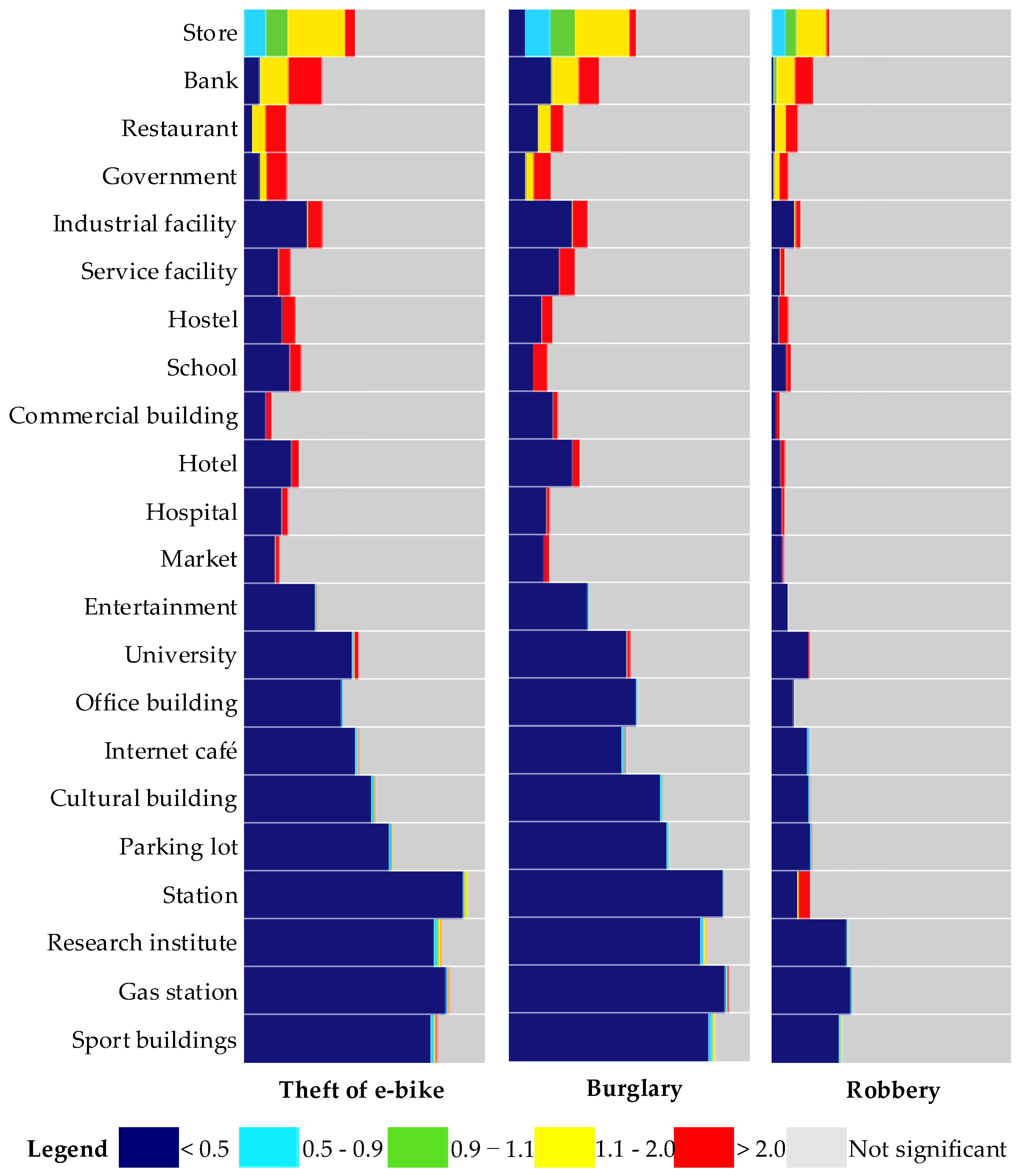
Due to the spatial homogeneity, individual crimes of the same type might be attracted to or deterred by land-use features at different levels of significance. To obtain an overview, we summarized the LCLQs between the types of crime and types of land-use features, illustrated as horizontal bars in Figure 4. The grey portion of each bar indicates the non-significant percentage of the LCLQs associated with the crimes and land-use features. The remaining colored portions represent the significant percentages (p < 0.01).
We classified the significant LCLQs into five groups based on the intensities (i.e., values of the LCLQ). Each group has been assigned a specific color for readability of the results. The dark blue portions of the bars in Figure 4 show the percentages of the LCLQs less than 0.5, which indicate a strong deterrence to crimes by the land-use features. The light blue portions of the bars (0.5 ≤ LCLQ ≤ 0.9) indicate weak deterrence, the green portion (0.9 < LCLQ < 1.1) indicates lack of influence, the yellow color (1.1 ≤ LCLQ ≤ 2.0) indicates weak attraction, and the red area (LCLQ > 2.0) indicates a strong attraction.
Figure 4 illustrates that the LCLQs of the three types of crime and the types of land-use features have similar structures. This similarity might be caused by the characteristics of these particular types of crime because all of them are property crimes that might be similarly influenced by land-use features.
However, particular types of crime are attracted to or deterred by different land-use features with different intensities. E-bike thefts were the most common of the three types of crimes. E-bikes offer inexpensive and convenient forms of transportation used by many residents, and they are particularly popular in families. People often ride e-bikes to work or for fun. E-bike thefts are likely to be found near stores, banks, restaurants, and governmental facilities. The overall local colocation patterns between e-bike theft and stores was hierarchal. Stores were the most common land-use feature of the 22 categories of land-use features. These stores are usually privately owned small shops that cater to relatively less affluent customers.
The crime dataset indicated that many victims had intended to temporarily park their e-bikes outside these stores. They had planned to buy something and shortly return to their e-bikes, so many of them left their e-bikes unlocked and forgot to monitor their bicycles while shopping. This carelessness provides opportunities for thieves. Banks are places where people routinely go to manage their money, ordinary restaurants are places where people go to dine, and governmental facilities are places where people conduct public or private business. These four types of land-use features are public places with large numbers of people that are difficult to regulate. This might partly explain why these land-use features attract e-bike thefts.
Only a small portion of industrial plants, service facilities, hostels, schools, commercial buildings, hotels, hospitals, markets, and universities strongly attracted e-bike thefts. The reason for that might be that few citizens traveled to these places by e-bike. In contrast, the remaining types of land-use features mainly deterred crime. These land-use features are either high-class places with security measures, including entertainment venues, office buildings, Internet cafés, cultural facilities, professional facilities, sports facilities, or places unlikely to park e-bikes, such as parking lots, transportation stations, and gas stations.
The local colocation patterns of burglaries with land-use features were similar to those of e-bike thefts. These two types are common property crimes with high exposure rates and low detection rates. Their similar spatial density distributions of crime are shown in Figure 2a,b above, which, along with their similar characteristics, might result in similar local colocation patterns. However, despite the overall similarity, there are differences. Stores, banks, restaurants, service facilities, commercial buildings, high-class hotels, office buildings, and cultural facilities had higher rates of strong deterrence to burglaries than they had to e-bike thefts. Most of these land-use features are in the middle and southern areas, where there is a large commercial center, a busy pedestrian street, and several scenic spots. These areas are mostly commercial sites, and the proportion of residences is low. Burglaries are crimes that occur in residential areas, and they are less likely to occur in commercial areas.
The local colocation patterns of robbery with land-use features clearly differed from those of e-bike theft and burglary. Overall, the percentages of significant LCLQs for robbery with individual types of land-use features were much smaller than for the other two types of crime. Moreover, different land-use features had different influences on robbery than on the other two types of crime. Stores, banks, and restaurants more strongly attracted robbery, which is a reasonable result because stores and restaurants are places with frequent cash transactions and cashiers and customers are potential victims. Bank employees and customers are easy targets for robbery because they tend to have money on hand. Governmental facilities attract robbery because they are responsible for some financial transactions involving cash, such as payment of water, electricity, heat, cable, and telephone bills.
Of note, a much larger percentage of transit stations invited robberies than e-bike thefts or burglaries. According to our data, almost 20% of all robberies in the study area during the study period were near bus stations, and 31 of them were near Hankou Railway Station. Bus stations are places where people gather, and the bustling crowd and lack of self-protection when getting on or off a bus provide opportunities for robbers. Hankou Railway Station is one of China’s most important railway hubs, located adjacent to Second Ring Road, surrounded by a large long-distance bus station and several local bus stations. The crowds of people in this area make it an ideal place for crime. However, the remaining types of land-use features mainly deterred robbery.
Another important benefit of using LCLQs is that the results are mappable, which provides the opportunity for visual interpretation and differences in the LCLQs can be observed over space. In other words, the spatial heterogeneity of the attraction/detraction intensities of the land-use features on crimes can be intuitively interpreted. Figure 5 presents maps of the local colocation patterns. To conserve space, four of the 22 types of land-use features are shown. Figure 5 shows that the colocation patterns of the types of crime and the types of land-use features were not homogeneous over space, which the global CLQ did not recognize.
A strong attraction of stores to e-bike thefts was mainly found in three areas, identified by the ovals numbered 1, 2, and 3 in Figure 5a. A large urban village with several wholesale markets and two main streets is located in area 1. Area 2 is the site of a large general hospital and a provincial bus terminal. The southern part of Jianghan District (Area 3) includes Hanzheng Street, which is a historically-prosperous center of trade. As shown in Figure 5d, banks attracted e-bike thefts mostly in the mid-southern and southern areas, which are the main commercial areas of the district.
Regarding restaurants’ attraction of e-bike thefts, there were three main areas, shown as the areas in ovals 4, 5, and 6 of Figure 5g. Wuhan No. 1 High School, the Party School of C. P. C. Wuhan Municipal Committee, and several communities are located in Area 4. Areas 5 and 6 are commercial areas, and there is a flourishing commercial pedestrian street in Area 6. Transit stations mainly presented a strong deterrence to e-bike theft (Figure 5j).
Figure 4 and Figure 5b,e,h,k illustrate that the influences of land-use features on burglary were similar to those on e-bike theft. However, Figure 5b shows that stores deterred burglary in the area inside oval 7. This difference was because several railways surround this area of crowded, shabby houses. The relatively poor transportation and economic conditions of this area are unlikely to encourage some types of land-use features, such as stores, banks, restaurants, and stations. On the other hand, the lack of public security measures provides opportunities for burglars. Overall, the land-use features strongly deterred burglaries in this area.
In contrast to e-bike theft and burglary, stores, banks, and restaurants mainly invite robbery. These influences tended to be distributed in the mid-southern and southern areas of the district, as shown in Figure 5c,f,i. However, Figure 5l, regarding transit stations, is clearly different because transit stations are far more attractive to robbery than to burglary or e-bike theft. Ovals numbered 8, 9, and 10 show three concentrated areas of attraction. Hankou Railway Station, a long-distance bus station, and several local bus stations are in area 8. Area 9 is between two parks, which are traversed from east to west by a main road. There is also a large department store in Area 9. Area 10 is the channel to a river-spanning bridge, and many bus transfer stations are located there. Area 10 is also near a dock, and it seems reasonable that these transportation hubs are places that should be protected from crime.
5. Conclusions
With the development of positioning technologies, information indicating where objects are placed is becoming more and more accessible. The study of space and place has become a crucial part of inter-disciplinary research such as that used by quantitative social scientists [43]. The improvement in computational power enables the adoption of sophisticated technologies for spatial analysis. This study explored the relationship between crime and land-use features from a spatial perspective. The adoption of spatial analysis tools provides a great opportunity to gain new scientific insights.
Through the analysis, we arrived at three main conclusions. First, colocation patterns of crime and land-use features obtained using the LCLQ were not stationary over space, and the global CLQ did not detect this spatial heterogeneity. Second, different types of land-use features had different influences on types of crime. Overall, stores, banks, restaurants, and governmental facilities invited the three types of crime observed in this study; industrial plants, service facilities, hostels, schools, commercial buildings, hotels, hospitals, markets, and universities mildly attracted crime; entertainment venues, office buildings, Internet cafés, cultural facilities, parking lots, research institutes, gas stations, and sport facilities deterred these types of crime. Third, some areas of the District stood out because distinct differences were found there. The mid-southern and southern areas are major commercial centers, and stores, banks, and restaurants strongly attracted crime. Transportation hubs were important because robberies tended to occur near them.
There are two key policy implications derived from this study. First, the mid-southern and southern areas were spatial criminal hot spots. These areas have complex demographic, economic, and geographical characteristics that need further governmental attention. Second, anti-crime measures should be conducted at the micro-level. To use the District’s limited police resources to effectively prevent crime, anti-crime patrols should be implemented in targeted areas. For example, stores, banks, restaurants, and governmental facilities were found in this study to be relatively more likely to attract e-bike theft and burglary, and transportation hubs attracted robbery. Instead of unorganized patrolling, police should focus on these places.
There are limitations associated with the methods used in this study. First, each land-use feature was represented as a point feature. However, some of these features covered large areas (e.g., industrial plants, markets, and universities). Simplifying polygons as points might produce a certain amount of deviation. For a more accurate assessment, other ways of studying the spatial relationships between points (e.g., crimes) and polygons (e.g., markets) could be employed [44]. Second, the global CLQ and the LCLQ do not consider edge effect. Without an edge effect correction, the colocation patterns between points near the boundaries of a study area tend to be biased. Since some of the neighbors to these points could be outside a study area, the actual number of neighbors might be underestimated. Various ways for resolving the problem, such as correcting factors, buffer zones, or toroidal duplication of the study area, could be borrowed from the edge effect correction of Ripley’s K function [45]. Third, the colocation quotient is a measure of the spatial association between the categorical subsets of points. Strictly speaking, the spatial association is not enough to expose the causal relationships between land-use features and crimes. Such causal inferences can be made with the help of cross-sectional studies [46].
Future work will focus on collecting environmental, economic, and demographic data. Factors, such as bar density, road density, police station density, bus station density, population density, and unemployment rates will be taken into account. Cross-sectional studies will be conducted to expose the causes of different types of crimes. The results from this research may help better interpret local variations in colocation patterns, and will serve to supplement and verify the findings of this study.
Acknowledgments
This research was funded by the following: the Open Fund of Key Laboratory of Police Geographic Information Technology, Ministry of Public Security (No. 2016LPGIT05); the Intelligent Supervision Platform of Wuhan Traffic Management Bureau; the Road Coding Information Spatialization System of Wuhan Traffic Management Bureau; and the National Science and Technology Pillar Program (grant no. 2012BAH35B03). The authors would like to thank Wuhan Municipal Bureau of Public Security for providing data for the research and Editage (www.editage.cn) for English language editing.
Author Contributions
Xinyue Ye conceived the idea for this research; Han Yue designed and performed the statistical analysis; Han Yue wrote major parts of the paper; and Xinyan Zhu and Wei Guo provided suggestions for the writing wrote minor parts of the paper and language-edited the final version of the manuscript. Authors have read and approved the final manuscript.
Conflicts of Interest
The authors declare no conflict of interest.
References
- Tobler, W.R. A computer movie simulating urban growth in the Detroit region. Econ. Geogr. 1970, 46, 234–240. [Google Scholar] [CrossRef]
- Leslie, T.F.; Frankenfeld, C.L.; Makara, M.A. The spatial food environment of the DC metropolitan area: Clustering, co-location, and categorical differentiation. Appl. Geogr. 2012, 35, 300–307. [Google Scholar] [CrossRef]
- Huang, Y.; Pei, J.; Xiong, H. Mining co-location patterns with rare events from spatial data sets. GeoInformatica 2006, 10, 239–260. [Google Scholar] [CrossRef]
- Arbia, G.; Espa, G.; Quah, D. A class of spatial econometric methods in the empirical analysis of clusters of firms in the space. Empir. Econ. 2008, 34, 81–103. [Google Scholar] [CrossRef]
- Leslie, T.F.; Kronenfeld, B.J. The colocation quotient: A new measure of spatial association between categorical subsets of points. Geogr. Anal. 2011, 43, 306–326. [Google Scholar] [CrossRef]
- Cromley, R.G.; Hanink, D.M.; Bentley, G.C. Geographically weighted colocation quotients: Specification and application. Prof. Geogr. 2014, 66, 138–148. [Google Scholar] [CrossRef]
- Sypion-Dutkowska, N.; Leitner, M. Land use influencing the spatial distribution of urban crime: A case study of Szczecin, Poland. ISPRS Int. J. Geo-Inf. 2017, 6, 74. [Google Scholar] [CrossRef]
- Wang, F.; Hu, Y.; Wang, S.; Li, X. Local indicator of colocation quotient with a statistical significance test: Examining spatial association of crime and facilities. Prof. Geogr. 2017, 69, 22–31. [Google Scholar] [CrossRef]
- Brantingham, P.J.; Brantingham, P.L. Environment, routine and situation: Toward a pattern theory of crime. Adv. Criminol. Theory 1993, 5, 259–294. [Google Scholar]
- Gabor, T. Situational crime prevention: Successful case studies. Can. J. Criminol. 1994, 36, 475–480. [Google Scholar]
- Brantingham, P.; Brantingham, P. Criminality of place. Eur. J. Crim. Policy Res. 1995, 3, 5–26. [Google Scholar] [CrossRef]
- Kinney, J.B.; Brantingham, P.L.; Wuschke, K.; Kirk, M.G.; Brantingham, P.J. Crime attractors, generators and detractors: Land use and urban crime opportunities. Built Environ. 2008, 34, 62–74. [Google Scholar] [CrossRef]
- Mccord, E.S. Intensity value analysis and the criminogenic effects of land use features on local crime patterns. Crime Patterns Anal. 2009, 2, 17–30. [Google Scholar]
- Frisbie, D.W.; Fishbine, G.; Hintz, R.; Joelson, M.; Nutter, J.M. Crime in Minneapolis: Proposals for Prevention; Governor’s commission on crime prevention and control: St. Paul, MN, USA, 1977.
- Roncek, D.W.; Bell, R. Bars, blocks, and crimes. J. Environ. Syst. 1981, 11, 35–47. [Google Scholar] [CrossRef]
- Roncek, D.W.; Maier, P.A. Bars, blocks, and crimes revisited: Linking the theory of routine activities to the empiricism of “hot spots”. Criminology 1991, 29, 725–753. [Google Scholar] [CrossRef]
- Gruenewald, P.J.; Freisthler, B.; Remer, L.; LaScala, E.A.; Treno, A. Ecological models of alcohol outlets and violent assaults: Crime potentials and geospatial analysis. Addiction 2006, 101, 666–677. [Google Scholar] [CrossRef] [PubMed]
- Grubesic, T.H.; Pridemore, W.A. Alcohol outlets and clusters of violence. Int. J. Health Geogr. 2011, 10, 30. [Google Scholar] [CrossRef] [PubMed]
- Livingston, M. A longitudinal analysis of alcohol outlet density and domestic violence. Addiction 2011, 106, 919–925. [Google Scholar] [CrossRef] [PubMed]
- Day, P.; Breetzke, G.; Kingham, S.; Campbell, M. Close proximity to alcohol outlets is associated with increased serious violent crime in New Zealand. Aust. N. Z. J. Public Health 2012, 36, 48–54. [Google Scholar] [CrossRef] [PubMed]
- Groff, E.; Mccord, E.S. The role of neighborhood parks as crime generators. Secur. J. 2012, 25, 1–24. [Google Scholar] [CrossRef]
- Demotto, N.; Davies, C.P. A GIS analysis of the relationship between criminal offenses and parks in Kansas City, Kansas. Cartogr. Geogr. Inf. Sci. 2006, 33, 141–157. [Google Scholar] [CrossRef]
- Ratcliffe, J.H.; Taniguchi, T.A. Is crime higher around drug-gang street corners? Two spatial approaches to the relationship between gang set spaces and local crime levels. Crime Patterns Anal. 2008, 1, 17–39. [Google Scholar]
- Kubrin, C.E.; Squires, G.D.; Graves, S.M.; Ousey, G.C. Does fringe banking exacerbate neighbourhood crime rates? Criminol. Public Policy 2011, 10, 437–466. [Google Scholar] [CrossRef]
- Chang, D. Social crime or spatial crime? Exploring the effects of social, economic, and spatial factors on burglary rates. Environ. Behav. 2011, 43, 26–52. [Google Scholar] [CrossRef]
- Isserman, A.M. The location quotient approach to estimating regional economic impacts. J. Am. Plan. Assoc. 1977, 43, 33–41. [Google Scholar] [CrossRef]
- Blair, J.P. Local Economic Development: Analysis and Practice; Sage: Newbury Park, CA, USA, 1995. [Google Scholar]
- Brantingham, P.L.; Brantingham, P.J. Location quotients and crime hot spots in the city. In Crime Analysis through Computer Mapping; Criminal Justice Information Authority: Chicago, IL, USA, 1993. [Google Scholar]
- Andresen, M.A. Location quotients, ambient populations, and the spatial analysis of crime in Vancouver, Canada. Environ. Plan. A 2007, 39, 2423–2444. [Google Scholar] [CrossRef]
- Zhang, H.; Peterson, M.P. A spatial analysis of neighbourhood crime in Omaha, Nebraska using alternative measures of crime rates. Internet J. Criminol. 2007, 31, 1–31. [Google Scholar]
- Pridemore, W.A.; Grubesic, T.H. A spatial analysis of the moderating effects of land use on the association between alcohol outlet density and violence in urban areas. Drug Alcohol Rev. 2012, 31, 385–393. [Google Scholar] [CrossRef] [PubMed]
- Kronenfeld, B.J.; Leslie, T.F. Restricted random labelling: Testing for between-group interaction after controlling for joint population and within-group spatial structure. J. Geogr. Syst. 2015, 17, 1–28. [Google Scholar] [CrossRef]
- Groff, E.; Weisburd, D.; Morris, N.A. Where the Action Is at Places: Examining Spatio-Temporal Patterns of Juvenile Crime at Places Using Trajectory Analysis and GIS; Springer: New York, NY, USA, 2009. [Google Scholar]
- Miller, H.J.; Han, J. Geographic Data Mining and Knowledge Discovery; CRC Press: Boca Raton, FL, USA, 2009. [Google Scholar]
- Silverman, B.W. Density Estimation for Statistics and Data Analysis; CRC press: Boca Raton, FL, USA, 1986. [Google Scholar]
- Bailey, T.C.; Gatrell, A.C. Interactive Spatial Data Analysis; Longman Scientific & Technical: Essex, UK, 1995. [Google Scholar]
- Anselin, L.; Cohen, J.; Cook, D.; Gorr, W.; Tita, G. Spatial analyses of crime. Crim. Justice 2000, 4, 213–262. [Google Scholar]
- Erdogan, S.; Yilmaz, I.; Baybura, T.; Gullu, M. Geographical information systems aided traffic accident analysis system case study: City of Afyonkarahisar. Accid. Anal. Prev. 2008, 40, 174–181. [Google Scholar] [CrossRef] [PubMed]
- Lahr, H. An improved test for earnings management using kernel density estimation. Eur. Account. Rev. 2014, 23, 559–591. [Google Scholar] [CrossRef]
- Ye, X.; Xu, X.; Lee, J.; Zhu, X.; Wu, L. Space–time interaction of residential burglaries in Wuhan, China. Appl. Geogr. 2015, 60, 210–216. [Google Scholar] [CrossRef]
- Townsley, M.; Homel, R.; Chaseling, J. Infectious burglaries. A test of the near repeat hypothesis. Br. J. Criminol. 2003, 43, 615–633. [Google Scholar] [CrossRef]
- Bembenik, R.; Rybiński, H. FARICS: A method of mining spatial association rules and collocations using clustering and Delaunay diagrams. J. Intell. Inf. Syst. 2009, 33, 41–64. [Google Scholar] [CrossRef]
- Goodchild, M.F.; Anselin, L.; Appelbaum, R.P.; Harthorn, B.H. Toward spatially integrated social science. Int. Reg. Sci. Rev. 2000, 23, 139–159. [Google Scholar] [CrossRef]
- Guo, L.; Du, S.; Haining, R.; Zhang, L. Global and local indicators of spatial association between points and polygons: A study of land use change. Int. J. Appl. Earth Obs. Geoinf. 2013, 21, 384–396. [Google Scholar] [CrossRef]
- Goreaud, F.; Pelissier, R. On explicit formulas of edge effect correction for Ripley’s K-function. J. Veg. Sci. 1999, 10, 433–438. [Google Scholar] [CrossRef]
- Liu, H.; Zhu, X. Exploring the influence of neighborhood characteristics on burglary risks: A Bayesian random effects modeling approach. ISPRS Int. J. Geo-Inf. 2016, 5, 102. [Google Scholar] [CrossRef]
Figure 1.
Jianghan District in Wuhan City.
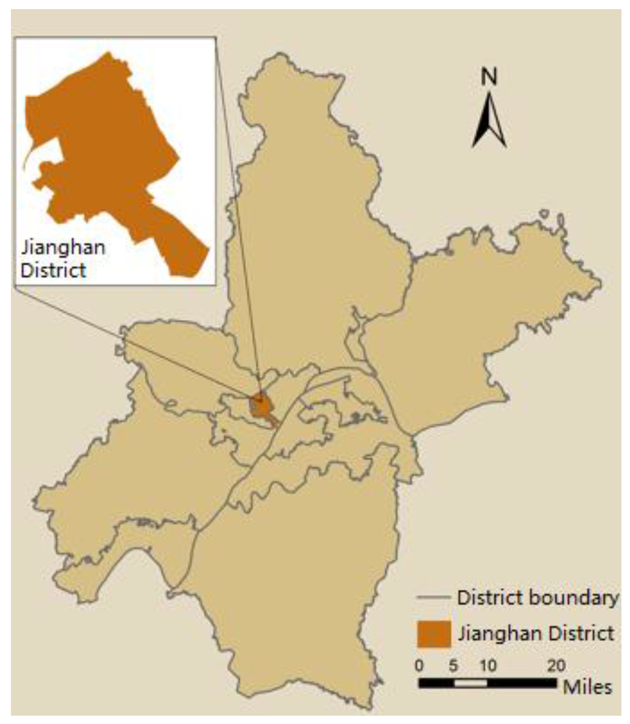
Figure 2.
Kernel density estimation of the three types of crime: (a) theft of e-bike; (b) burglary; and (c) robbery.
Figure 2.
Kernel density estimation of the three types of crime: (a) theft of e-bike; (b) burglary; and (c) robbery.
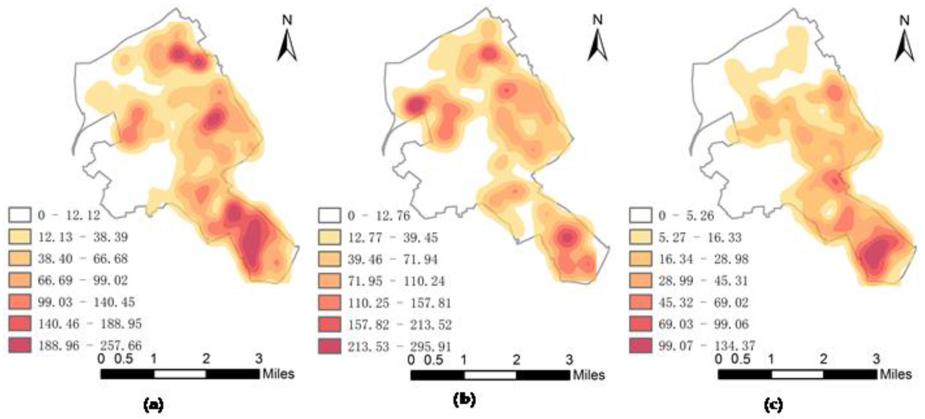
Figure 3.
Hourly ratios of crimes: (a) theft of e-bike; (b) burglary; and (c) robbery.
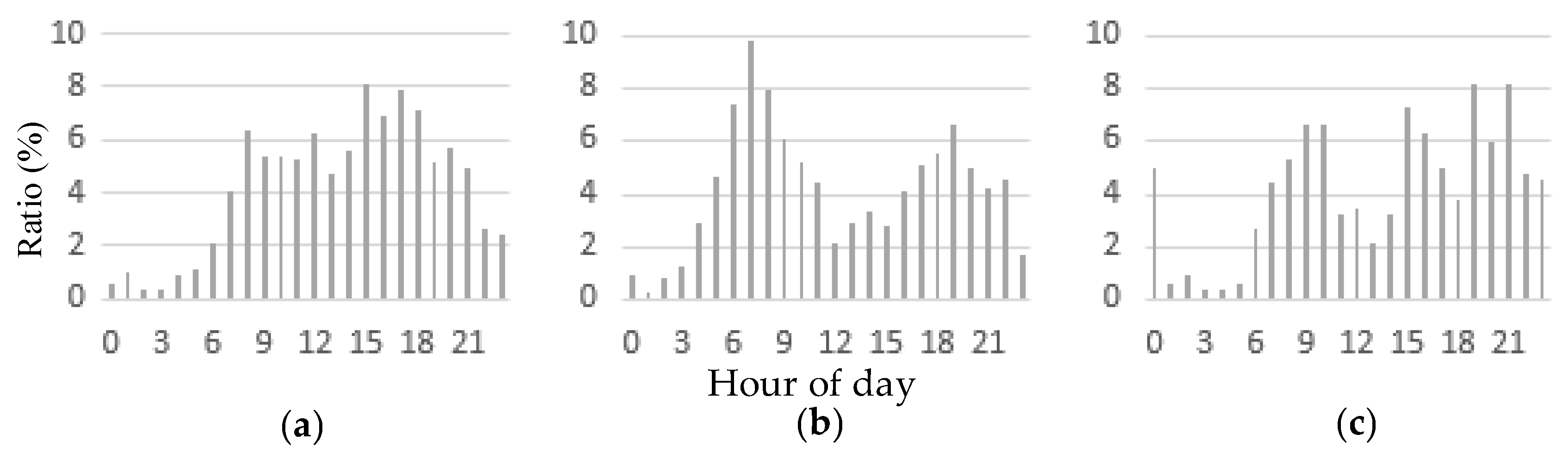
Figure 4.
LCLQ comparisons among types of crime and types of land-use feature.

Figure 5.
Maps of local colocation patterns of crimes and land-use features for stores, banks, restaurants, and stations: (a) theft of e-bike and store; (b) burglary and store; (c) robbery and store; (d) theft of e-bike and bank; (e) burglary and bank; (f) robbery and bank; (g) theft of e-bike and restaurant; (h) burglary and restaurant; (i) robbery and restaurant; (j) theft of e-bike and station; (k) burglary and station; (l) robbery and station.


Table 1.
Reclassified land-use feature types, numbers of cases, and original types.
| Type | Reclassified Land-Use Feature | n | Original Land-Use Feature Types in the PGIS Geo-Database |
|---|---|---|---|
| 1 | Store * | 1030 | Clothing store, grocery store, flower shop, pharmacy, electronics store, bookstore, pastry shop, bird market, cosmetics store, building materials store, grain and oil store, farmer’s market, musical instrument shop, fruit and vegetable market, office supply store, liquor store, eyeglasses store, jewelry store, and others |
| 2 | Bank | 593 | Bank, ATM |
| 3 | Restaurant | 481 | Restaurant, Chinese tea house, fast food restaurant, coffeehouse, Western cuisine restaurant |
| 4 | Government | 420 | Governmental office, police station, surveillance room, and others |
| 5 | Industrial facility | 310 | Electronics equipment factory, machine factory, motor vehicle manufacturer, garment factory, textile mill, furniture factory, food factory, industrial park, chemical plant, metal factory, wood factory, plastics plant, rubber factory, paper mill, and others |
| 6 | Service facility | 278 | Barbershop, beauty shop, laundry, photo studio, and others |
| 7 | Hostel | 268 | Hostel, private hotel |
| 8 | School | 267 | Kindergarten, primary school, middle school |
| 9 | Commercial building | 241 | Trading company, communications company, logistics company, postal corporation, warehouse, power facility, fuel gas facility, water supply facility, and others |
| 10 | Hotel | 233 | Five-star hotel, four-star hotel, three-star hotel, unrated hotel |
| 11 | Hospital | 208 | General hospital, special hospital, clinic, community health station, epidemic prevention station |
| 12 | Market * | 202 | Supermarket, small market, mid-sized market, shopping center, bazaar, and others |
| 13 | Entertainment | 126 | Massage parlor, nightclub, Karaoke club, video game entertainment center, and others |
| 14 | University | 109 | University, university for the elderly, vocational school |
| 15 | Office building | 106 | Office building |
| 16 | Internet café | 81 | Internet café |
| 17 | Cultural building | 70 | Museum/art gallery, newspaper office, television station, cultural palace, library, and others |
| 18 | Parking lot | 63 | Parking lot |
| 19 | Station | 39 | Railway station, bus station, taxi stand, dock |
| 20 | Research Institute | 29 | Scientific research institution, science park, and others |
| 21 | Gas station | 25 | Gas station |
| 22 | Sport buildings | 24 | Gymnasium, fitness center, and others |
* The differences between stores and markets are described briefly in terms of three aspects as follows: (1) size (a store is small, but a market is large); (2) ownership (generally, a store is privately operated, but a market is public-owned); and (3) varieties of the commodities sold (stores typically sell a single species of goods, whereas markets sell various kinds of commodities).
Table 2.
Average distance between crimes and land use features.
| Type of Crime | Average Distance between Each Type of Crime and nth Nearest Neighborhood (m) | ||
|---|---|---|---|
| n = 1 | n = 10 | n = 20 | |
| Theft of electric bicycle | 39 | 115 | 163 |
| Burglary | 49 | 142 | 192 |
| Robbery | 34 | 124 | 186 |
Table 3.
Global colocation quotients of three types of crimes and land-use features.
| Land-Use Feature Type | E-Bike Theft | Burglary | Robbery |
|---|---|---|---|
| Store | 0.91 | 0.76 * | 0.89 |
| Bank | 0.87 * | 0.67 * | 0.99 |
| Restaurant | 0.71 * | 0.72 * | 0.59 * |
| Government | 0.82 * | 0.8 * | 0.83 * |
| Industrial facility | 0.72 * | 0.47 * | 0.66 * |
| Service facility | 0.38 * | 0.28 * | 1.23 * |
| Hostel | 0.9 * | 0.87 * | 0.86 * |
| School | 0.85 * | 0.83 * | 1.08 |
| Commercial building | 0.9 * | 0.47 * | 0.94 |
| Hotel | 1.01 | 0.62 * | 1.27 * |
| Hospital | 0.97 | 0.94 | 0.87 * |
| Market | 0.82 * | 0.62 * | 0.88 * |
| Entertainment | 0.88 * | 0.65 * | 1.15 * |
| University | 0.88 * | 0.94 * | 0.69 * |
| Office building | 0.88 * | 0.78 * | 0.78 * |
| Internet café | 0.73 * | 0.63 * | 0.47 * |
| Cultural building | 0.94 | 0.92 * | 0.96 |
| Parking lot | 0.95 | 0.7 * | 1.12 * |
| Station | 0.86 * | 0.79 * | 0.96 |
| Research Institute | 0.81 * | 0.82 * | 0.87 * |
| Gas station | 0.84 * | 0.78 * | 0.93 * |
| Sport buildings | 0.97 | 0.94 * | 0.85 * |
* p < 0.01.
© 2017 by the authors. Licensee MDPI, Basel, Switzerland. This article is an open access article distributed under the terms and conditions of the Creative Commons Attribution (CC BY) license (http://creativecommons.org/licenses/by/4.0/).
Share and Cite
MDPI and ACS Style
Yue, H.; Zhu, X.; Ye, X.; Guo, W. The Local Colocation Patterns of Crime and Land-Use Features in Wuhan, China. ISPRS Int. J. Geo-Inf. 2017, 6, 307. https://0-doi-org.brum.beds.ac.uk/10.3390/ijgi6100307
AMA Style
Yue H, Zhu X, Ye X, Guo W. The Local Colocation Patterns of Crime and Land-Use Features in Wuhan, China. ISPRS International Journal of Geo-Information. 2017; 6(10):307. https://0-doi-org.brum.beds.ac.uk/10.3390/ijgi6100307
Chicago/Turabian StyleYue, Han, Xinyan Zhu, Xinyue Ye, and Wei Guo. 2017. "The Local Colocation Patterns of Crime and Land-Use Features in Wuhan, China" ISPRS International Journal of Geo-Information 6, no. 10: 307. https://0-doi-org.brum.beds.ac.uk/10.3390/ijgi6100307
Note that from the first issue of 2016, this journal uses article numbers instead of page numbers. See further details here.