Extraction of Road Intersections from GPS Traces Based on the Dominant Orientations of Roads

Abstract

Many studies have used Global Navigation Satellite System (GNSS) traces to successfully extract segments of road networks because such data can be rapidly updated at a low cost. However, most studies have not focused on extracting intersections, which are indispensable parts of road networks in terms of connectivity. However, extracted intersections often present unsatisfactory precision and misleading connectivity. This study proposes a novel method for extracting road intersections from Global Position System (GPS) trace points and for capturing intersections with better accuracy. The key to improving the geometric accuracy of intersections is to identify the dominant orientations of road segments around intersections, merge similar orientations and maintain independent conflicting orientations. Extracting intersections by aligning the dominant orientations can largely reduce location offsets and road distortions. Experiments are performed to demonstrate the increased accuracy and connectivity of extracted road intersections by the proposed method.

1. Introduction

Road networks are the basic geographic information that constitute urban structural skeletons and connect various geographic elements in a city, and they play key roles in vehicle navigation, traffic management, and rapid emergency responses [1]. Maintaining timely information on road networks [2], especially in developing cities where road networks may change rapidly, is challenging. Conventional ground-based survey map updating techniques are restricted because of the long periods required to collect and organize geographic information [1]. Remote sensing interpretations can be used to extract road maps but cannot capture large-scale and complex road networks, and are affected by occlusions caused by clouds, mist and trees.

Public vehicles with Global Navigation Satellite System positioning devices make it possible to continuously probe the dynamics of city traffic statuses with complete coverage [3]. However, vehicle movement, building blockages, high-noise trajectories, outliers and limited-resolution GNSS equipment cause pervasive position deviations in GNSS trajectory data [4,5]. This new geospatial resource nevertheless contains a wealth of generic information related to road networks, road grades, traffic conditions and driving behaviour [6]. For a vehicle trajectory with a positioning accuracy of 5–20 m [7], even the location accuracy of a single trajectory point is very low, most of the random errors can be eliminated between a large number of trajectory points in the local range. Therefore, the use of these low-quality tracking data to extract high-quality road maps is a hot topic [7]. Compared with traditional procedures used to produce road networks, a map inference approach can fully exploit the spatiotemporal information generated by tracking data, thereby enabling users to extract and update road networks over shorter periods.

However, updating a road network starts from the premise that the coordinates of the extracted road network are registered using intersections as control points [8], and the accuracy of intersection locations determines the resulting road network registration. Road intersections also play an important role in the road networks. They can provide very useful information, such as connectivity, topology and orientation. Based on the complete extracted road network, we can further analyse the preferences of the travellers on route selection [9], the commute between different transportation modes [10], traffic flow on the roads [11], the delays caused by traffic jams [10], and so forth. By comparing existing methods for road extraction, Cao et al. noted issues associated with these methods, namely, that these existing methods are unable to simultaneously achieve high precision and recall [7], especially for detecting intersections. Most of these methods focus on extracting road segments and treat intersections as points at which roadways are connected rather than distinguishing intersection types as a premise. Therefore, the existing road extraction methods could not extract all intersections with high geometric and road orientation accuracy; thus, the precise geometry and correct topology of the road networks could not be guaranteed.

To overcome these defects, an intersection extraction method is proposed in this work, and it uses the mean-shift clustering method to trace road segments to acquire accurate road orientations, and the dominant orientations of roads around the same intersection are identified and then used to determine the positions of the road intersections. The remainder of this paper is organized as follows. Section 2 presents related work regarding road and intersection extraction methods. Section 3 describes the method’s flow and the strategy used to extract intersections. Section 4 presents comparisons between two experimental Global Position System trace datasets and existing methods. Section 5 discusses the conclusions and suggestions for further work.

2. Related Work

Traditionally, remote sensing imagery is most often used to rapidly and economically acquire road segment and intersection data [12]. To extract centrelines accurately, Unsalan et al. [13] developed a flexible combinatorial method that relied on probabilistic and graph theory to detect and extract road networks. Boichis et al. assessed an interpretation strategy system for automatically extracting road intersections from aerial images [14]. Furthermore, Hu et al. proposed a toe-finding algorithm based on rectangular approximations to generate a road network and road intersections from aerial images [15] and discussed classical road intersection types. Unfortunately, frequent cloud cover and complicated pre-treatments (e.g., geometrical rectification and image mosaics) can have a cumulatively negative effect and even result in extracted road networks with errors in their topological structures.

With the widespread development of GNSS positioning devices embedded in smartphones and portable devices, GNSS trajectories are considered an emerging data source (comparing favourably with remote sensing images) for acquiring road networks [16]. Various methods have been developed to explore the impacts of GNSS tracking data issues on road extraction over past decades [7], and these methods can be categorized as point clustering methods, trace merging-based methods and intersection linking methods. In these novel approaches, the algorithms used to generate intersections from vehicle trajectories can be divided into two types.

One type directly extracts intersections using the local spatial characteristics of trajectory points or the spatial relationships between multiple trajectories at intersections. Fathi et al. [17] developed a classifier that was trained using shape descriptors from two temporally adjacent GPS points from the same vehicle to extract road intersections. Ahmed et al. [18] reconstructed intersections by utilizing sets of vertices within bounded regions (vertex regions), with regions bounded by the minimum incident angle of the streets at that intersection. Based on sparse GPS trace points, Wu et al. [19] converged low-quality raw points using Kernel Density Estimation (KDE) to identify cluster centres as intersection points. Xie et al. [20] extracted intersections using the inverse distance-weighted clustering method, and intersection points were identified from GPS points with changing directions. Wang et al. [21] identified intersections using a mean-shift algorithm to calculate the location of an intersection for which the neighbouring roads presented high turn density values.

The other type of algorithm detects roadways from trajectories and produces intersections by connecting the centrelines of roads. Davies et al. employed a contour Voronoi diagram to calculate road segments and intersections, and their method identifies pairs of nearby intersections that should merge [22]. Xie et al. detected the longest non-consecutive subsequences using dynamic programming and partitioned them into consecutive sub-tracks [23] to extract road intersections. Tang et al. used a heading criterion and topology extraction method to derive topology points, although their method cannot be applied to the geometries of complex junctions [24].

The first class of algorithms is based on the local spatial characteristics of trajectories in which vehicles stop more often and points are observed at a high frequency. However, vehicles stop at traffic lights and stop/yield signs and do not stop at the centres of intersections. The second type of algorithm connects the road centrelines at the same intersection at the mean point of the segment end node; however, the spatial relation between the road centrelines cannot be specified. Most of the methods mentioned above produce spurious and distorted intersections from vehicle GNSS traces.

Yao et al. [25] proposed a method that traces road orientations and intersections to refine the positions of road intersections from raster maps. Based on their study, in this work, we propose a new method to extract road intersections. The primary contributions of our method can be summarized as follows: the centrelines of the road were extracted from GPS trace points using a mean-shift clustering algorithm with penalty, which is robust for outliers and noise. Then, a principal component analysis (PCA) and depth-first search strategy were used to individually reconstruct the road segments, which avoid generating short branches. Using the centrelines of the road segments, we first employed what is termed a merge and intersect strategy for road segments at the same intersection to avoid intersection position deviations and road distortions. The smooth segments produced during merging were used to extract an average track, which acted as a geometric representation of each dominantly oriented segment, and these segments were then utilized to detect the locations of the intersections from independent dominant orientations.

3. Proposed Method

Road segments and intersections are fundamental elements of road networks. Road segments are connected by intersections; thus, the road intersections locations or positions, road connectivity and road orientations are the basic properties of intersections. In general, vehicles moving along different roads connected from different orientations form the influx at the intersections, and their locations can be inferred by the intersections of the dominant orientations of the road segments around intersections.

3.1. Road Skeleton Extraction

Because intersections are influxes of road segments, road segments should be extracted from collected GNSS points before identifying the intersection nodes of a road network. Currently, many methods are available to extract road segments, including hierarchical clustering and spectral clustering [26]; however, these methods cannot be used to process large amounts of data because of the requisite large number of calculations. Density-based approaches, in which Density-Based Spatial Clustering of Applications with Noise (DBSCAN) [27] and mean-shift algorithms [28] are employed, are preferred because dynamic cells are used to manipulate data within a neighbourhood. The mean-shift algorithm was used in this work because it captures the local maximum density positions of cells. However, DBSCAN merges proximal high-density cells into clusters.

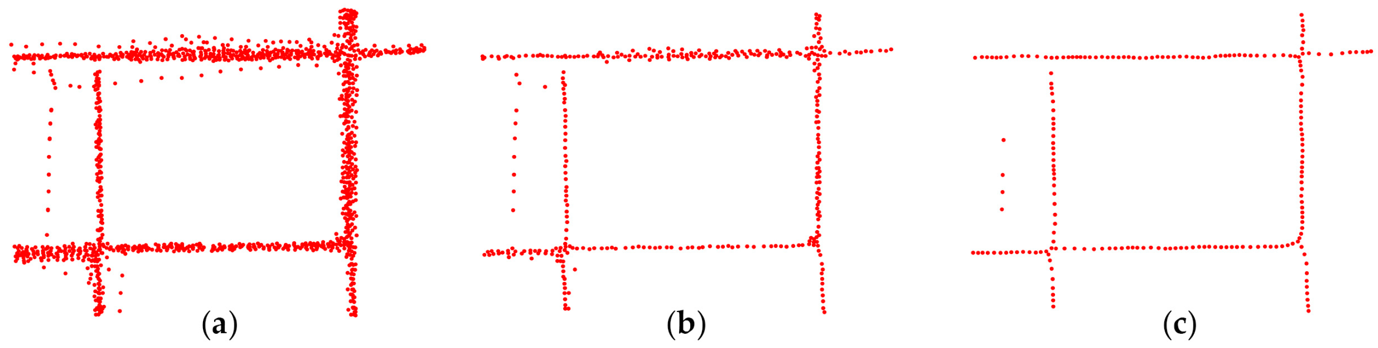
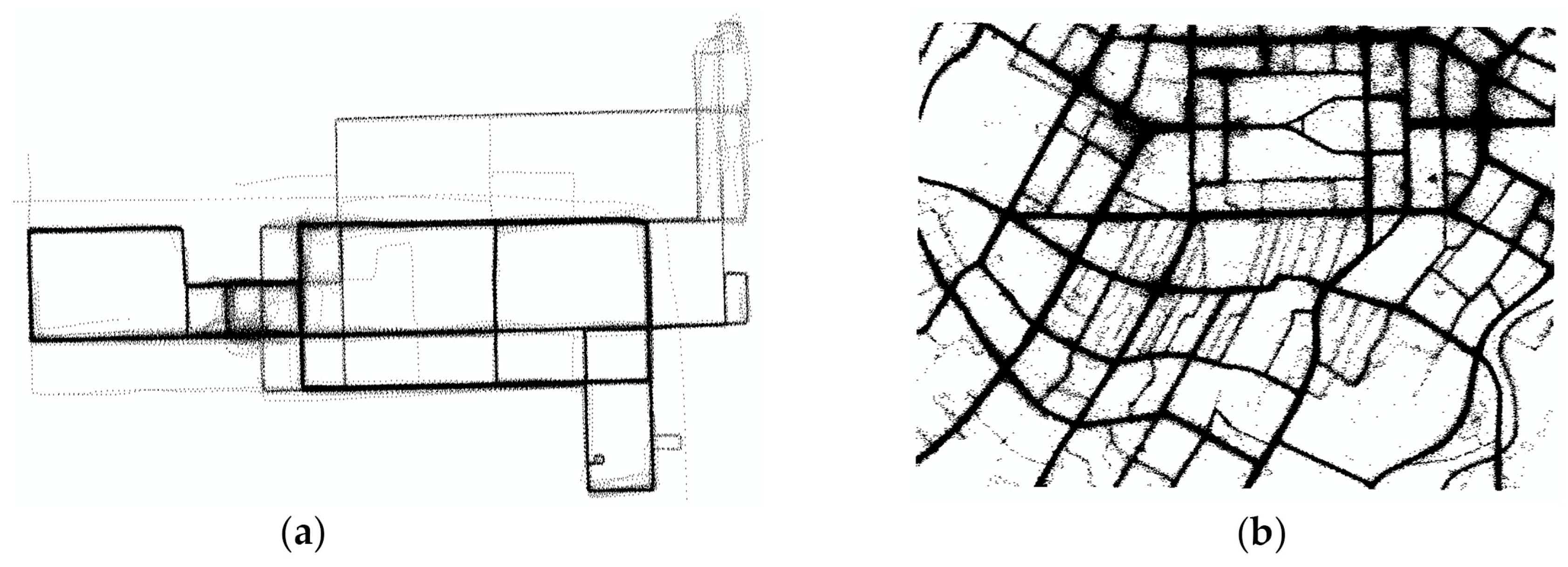
3.1.1. Simplification of Scattered Points

Mean-shift is a mode-seeking algorithm that searches for the maximum densities of local neighbourhoods from discrete points [29]. The algorithm is iterated until a stable result is obtained, that is, until a certain number of iterations is reached or all points move to the location of the local maximum density in the support neighbourhood. The employed version of the regularized mean-shift formula is

$$x_i^{k+1}=\frac{{{\displaystyle \sum }}_{j\in J}{q}_j^k{\alpha }_{ij}^k}{{{\displaystyle \sum }}_{j\in J}{\alpha }_{ij}^k}+\lambda \frac{{{\displaystyle \sum }}_{i\prime \in I\backslash \left\{i\right\}}\left(x_i^k-x_{i\prime }^k\right){\beta }_{ii\prime }^k}{{{\displaystyle \sum }}_{i\prime \in I\backslash \left\{i\right\}}{\beta }_{ii\prime }^k}.$$

(1)

where the first item is the classical mean-shift algorithm; the second item is a regularized term to prevent further accumulation once points are already contracted onto their local centre positions; $\lambda$ is balancing constants between the two item; ${\alpha }_{ij}=\theta \left(\Vert x_i-q_j\Vert \right)/\Vert x_i-q_j\Vert ;j\in J;{\beta }_{ii\prime }=\theta (\Vert x_i-x_{i\prime }\Vert )/\Vert x_i-x_{i\prime }{\Vert }^2;i\prime \in I\backslash \left\{i\right\}$; $\theta (\Vert .\Vert )=e^{-\Vert .{\Vert }^2/R^2}$ is a Gaussian smooth weight with a set neighbourhood radius R, and $\Vert .\Vert$ is the Euclidean distance between two points; $x_i^k$ is the initial position at the current iteration; and $x_i^{k+1}$ is the new position for one iteration loop with a support cell radius R. $q_j^k$ and $x_{i\prime }^k$ are the original and sampling points in the local neighbourhood of $x_i^k$ for the current iteration, respectively.

Using the above formula, the mean-shift algorithm clusters the sampling points based on the resampling of the original point. To accelerate the point clustering, when the distance of two sample points is less than 1 m, the two points are replaced by a point at their average position. Hence, the number of sampling points decreases with iterative calculations until only a few feature points remain, which are finally distributed at the local intermediate positions of the original GNSS track points, as illustrated in Figure 1.

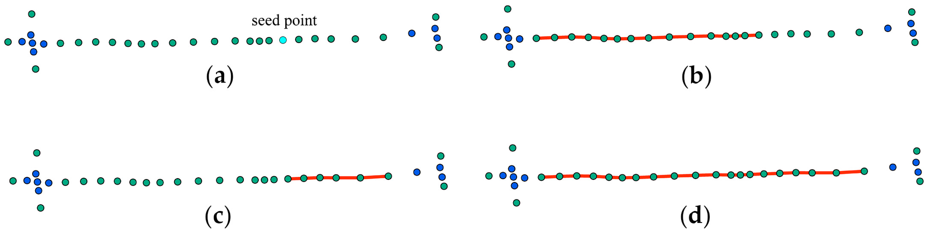
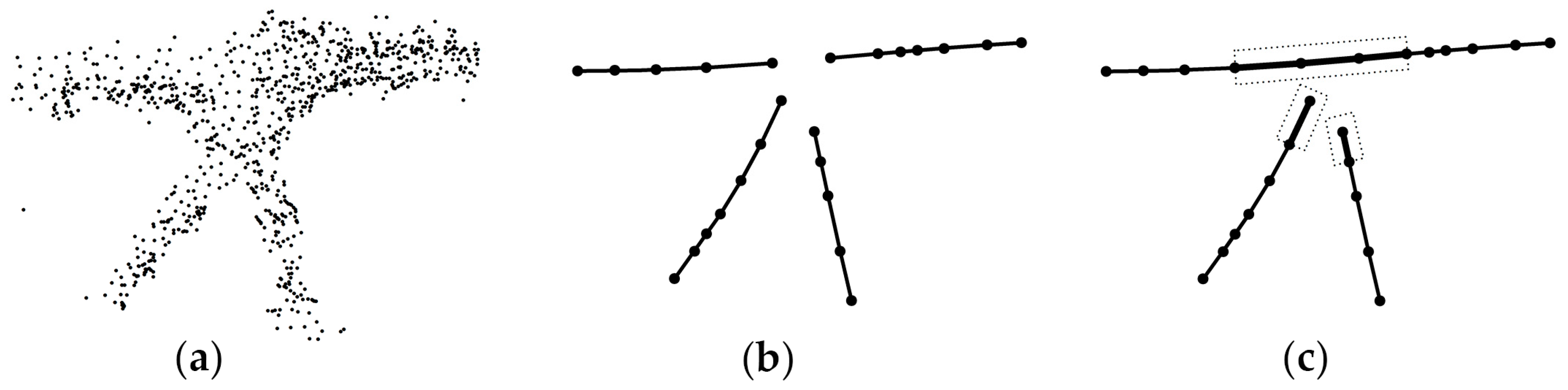
3.1.2. Road Skeleton Segmentation

Although feature points are evenly distributed in the middles of the roads, as shown in Figure 1c, they remain discrete. A classical PCA [30] was used to calculate the distribution characteristics of each of the feature points. A weighted covariance matrix $C_i={\left(x_i-x_{i\prime }\right)}^{\mathrm{T}}\left(x_i-x_{i\prime }\right)$ was calculated for feature point $x_i$ (a row vector) and the other feature points within its neighbourhood, and the eigenvalues $\left\{{\lambda }_i^0,{\lambda }_i^1\right\}$ and corresponding eigenvectors $\left\{e_i^0,e_i^1\right\}$ of the 2 × 2 covariance matrix $C_i$ were then calculated. The eigenvalues represent the degree of discretization of the feature points in the corresponding eigenvectors. The value ${\kappa }_i=max\left\{{\lambda }_i^0，{\lambda }_i^1\right\}/\left({\lambda }_i^0+{\lambda }_i^1\right)$ is then defined as the linearity degree of $x_i$ within the local neighbourhood at radius R. The difference between the two eigenvalues is smaller, indicating that the distribution of points in the direction of the corresponding eigenvectors is equivalent, and the value of ${\kappa }_i$ is closer to 0.5. On the contrary, the maximum eigenvalue is far greater than the other, and more points around $x_i$ are aligned along a direction, and the value of ${\kappa }_i$ is closer to 1. Hence, the ${\kappa }_i$ values range from [0.5, 1]. If the ${\kappa }_i$ values are close to 1, then the points have more linear distributions, which means that more of the feature points around $x_i$ are aligned along a road. However, if the ${\kappa }_i$ values are closer to 0.5, then the distribution is more uniform. Therefore, the candidate points (green dots) used to generate road segments are selected from the feature points with ${\kappa }_i$ > 0.9 as shown in Figure 2a.

To identify road segments from those candidates, the seed point with the largest $k$ value, $p_0$, is first selected. For the seed point, the depth-first search strategy [31] is used to trace the next seed point to nearby candidates along the dominant PCA direction $e_p$. To avoid straddles the intersection or connecting to the adjacent road during the road segment search process, this strategy requires the following two parameters: $dis\left(p_0,x_i\right)<30,i=0,1,2\dots$ and $\angle \left(e_p,\left(x_i-p_0\right)\right)<15°,i=0,1,2\dots$ [32]. These parameters were determined based on the lane width and the number of real urban roads as well as much experimental exploration to yield the best results for the tracking data. The lane width in the cities is approximately 3.5~4.0 m, and we assume that the roads that the vehicles visited contained at least four lanes. In addition, road barriers and the buffer zone at the intersection should also be taken into account. The second parameter was set at 15°, meaning that the road segment was not allowed to track a connection to another road near the intersection area or parallel to itself. By replacing $x_i$ with $p_0$, nearby candidate points are searched via the same method, and stops are traced when none of the candidate points in the local neighbourhood satisfy the above conditions. Correspondingly, the direction opposite the dominant PCA direction of the original seed point can also be searched to identify another path, and the results of the two paths are then merged into one road segment as illustrated in Figure 2. If at least five candidate points (by default) are found during the trace, then those points are labelled as road nodes and are connected to generate road segments [31]. The process is repeated with a new seed point with the largest $k$ among the remaining candidates until all the candidate points are processed.

3.2. Orientation-Based Extraction of Intersections

Intersections are commonly known as junctions when two or more roads intersect or meet each other. Intersections are classified as 2-way, 3-way, 4-way, or 5-way, and so on, depending on the number of road segments (road connectivity) that meet at the same intersection. The morphology of a road may be distorted when an intersection node is formed directly by connecting more road segments or by the mean value of road segment end nodes. Figure 3b illustrates the distortions of T-shaped road intersections, which were connected using the mean value of the coordinates. To overcome these distortions, the approximately collinear segments near the intersection are identified and merged, and the location of the intersection is extracted from those conflicting orientations to extract more accurate road intersections.

Koutaki et al. provided three intersection models according to the road width and orientation including: the crossroads model, which represents the intersection of two road portions; the three-forked road model, which has three road segments; and the T-intersection model, which consists of one straight road and a connected branch [33]. However, their models are not suitable for roads with arbitrary incidence angles at intersections. To apply more intersection geometry types and variable orientations, stronger constraints and additional knowledge regarding intersections should be refined. Because intersections with the same road connectivity can be intersected with diverse forms associated with road segments with different independent dominant orientations [34], a set of paired segments that are approximately collinear is first identified around the same intersection. Each pair is merged into a single segment and, finally, only the conflicting orientation segments at the same intersection are retained. Here, conflicting does not necessarily mean that there is a 90° difference in orientation from a reference orientation, but rather that the orientation differs greatly from the reference, which is defined as the independent dominant orientation of the intersection. Therefore, intersection locations can be detected by finding nearby road segments at the same intersection that intersect in multiple conflicting orientations. Under that assumption, a two-step strategy that merges collinear segments and intersecting conflicting segments is proposed for detecting the locations of intersections.

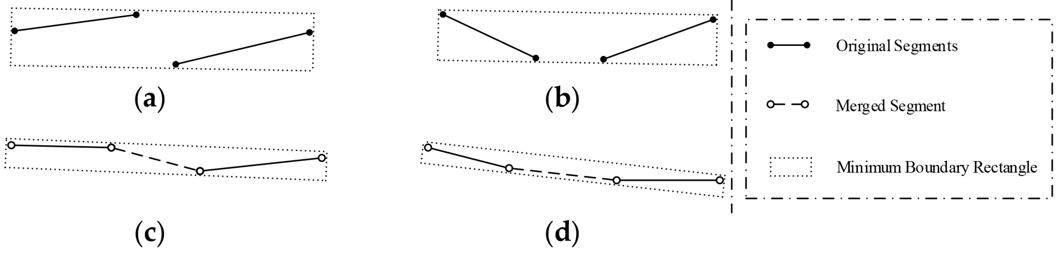
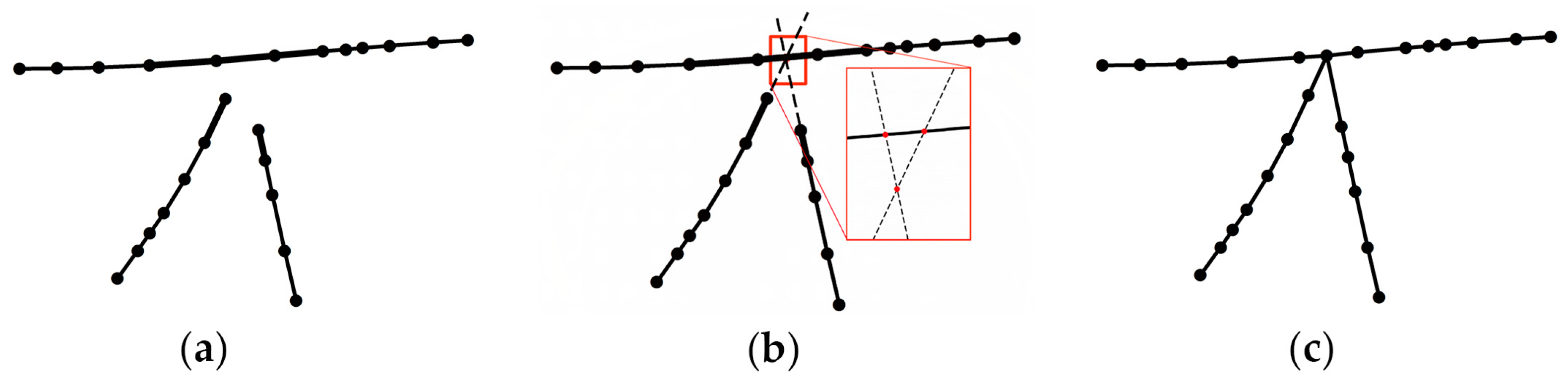
3.2.1. Identification of Collinear Segments

Roads have characteristics of compactness, parallelism, convexity and ductility [35]. Regnauld [36] and Campbell [37] used parallelism and compactness as the main factors to select road networks for generalizing maps. In this work, a spatial feature measure function called Cost, which is the degree of collinearity based on parallelism and compactness, is proposed to analyse the spatial relationship between pairwise segments around the same intersection, where the segments exhibit collinearity that is not necessary strictly 0° or 180°, but have approximate orientations. The cost function Cost is defined as

$$Cost=\sqrt{Parallelism\times \left(1-Compactness\right)},$$

(2)

$$Parallelism=\frac{2Length-MBR}{Perimeter},$$

(3)

$$Compactness=4\pi \times \frac{Area}{Perimete{r}^2},$$

(4)

where Length-MBR is the length of the longest edge of the minimum boundary rectangle (MBR) of the geometry and Perimeter and Area represent the perimeter and area of the geometry, respectively. In this work, the segments refer to the end segments of road segments around the same intersection, and the MBR of any two segments is used as the geometry.

Parallelism and Compactness range from 0 to 1. Parallelism increases with thinner MBR, and Compactness is conversely related to Parallelism because long and thin geometries are not compact. Cost ranges from 0 to 1, and if the Cost is close to 1, two road segments are more collinear along one orientation, and if the Cost is close to 0, two road segments are spatially distributed along two independent and dominant orientations.

The two candidate segments with the larger aggregation Cost are chosen and merged if the Cost is larger than a minimum threshold. Guillaume et al. [38] used 0.83 and 0.2 as thresholds for parallelism and compactness (the corresponding calculated value of Cost is 0.81), respectively, to select the main road in a map generalization. However, these authors used the two criteria as the measures for a complete road, whereas in this work, only parts of road segments are calculated. After a series of experiments, the Cost threshold was set to 0.85 so that two segments could be aligned to the similar orientation. As illustrated in Figure 4, a group of road segments with different spatial distributions were chosen as candidates (only the end segment of a road around the intersection is illustrated), where the solid line represents the extracted road in Section 3.1.2, and the dotted line represents the refitted results. As shown in Figure 4a,b, the Cost of the two candidate neighbours was less than the set threshold, and the candidates were considered to have two dominant orientations and no modifications. Figure 4a presents two segments that are spatially parallel but not collinear. Figure 4b shows two segments that are said to be conflicting in the two independent orientations, which should persist until the following step. However, as shown in Figure 4c,d, these segments have greater Cost values, which indicates that they are regarded as a broken road with similar orientations that should be merged into a smooth segment.

A set of mutual conflicting road segments was therefore obtained around the same intersection and included two types, one of which was the original and independent segments, and the other was refitted by merging a pair of approximately collinear segments. The two types of segments both are hereafter considered independent of conflicting segments. Figure 5 presents the results of the collinear identification and shows three conflicting segments around the intersection after the merge operation.

3.2.2. Detecting the Locations of Intersections

From the above collinear identification and segment merging process, a set of conflicting segments with conflicting orientations around the same intersection were acquired, as shown in Figure 5c or Figure 6a. However, the location of the actual intersection could not be determined using the intersections of those segments at the same intersection because more than one intersection may occur, as shown in Figure 6b. In this step, the intersections of the conflicting road segments are first calculated, as shown in Figure 6b, and then the actual location of the intersection is calculated, which illustrated in Figure 6c.

As illustrated in Figure 7, the intersections were calculated from different road connectivity (end segments of road segments) and spatial relationships. Three intersecting cases are possible for the road segments around the intersection.

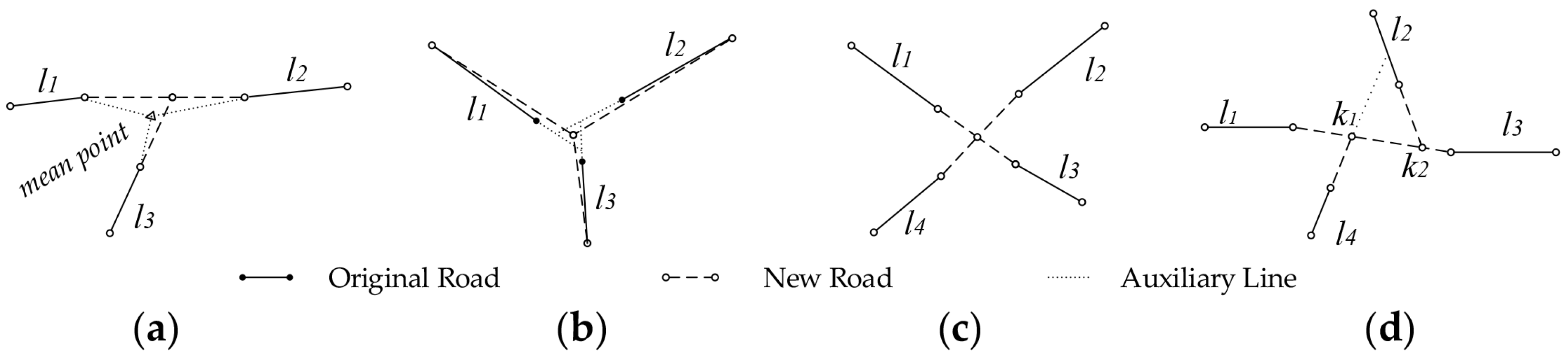
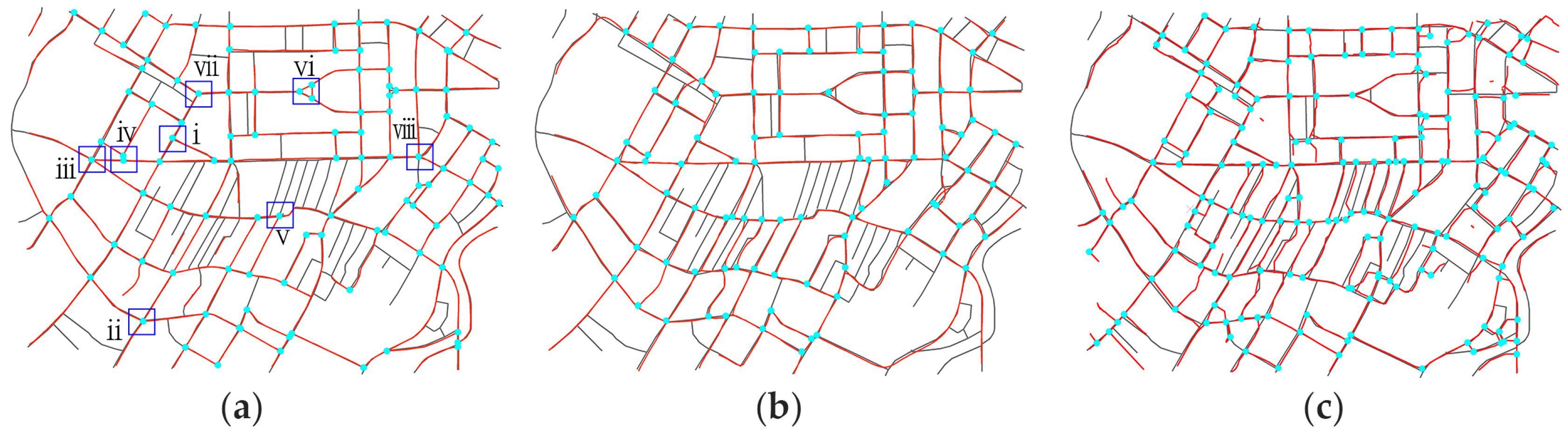
• In the first case, all the segments intersect at one point exactly, as illustrated in Figure 7a,c.
• In the second case, the segments intersect at multiple sub-intersections and the sub-intersections are all near the road intersection position, as illustrated in Figure 7b.
• In the third case, the segments intersect at multiple sub-intersections but some of the sub-intersections are not near the road intersection (i.e., outliers and noise), as illustrated in Figure 7d.

Generally, intersections are sufficiently far apart that their buffers do not superimpose. However, for sub-intersections that are part of a splintered larger intersection, which frequently occur over a small distance, calculating the distance between the adjacent sub-intersections could help determine the intersections that are correlated and should be merged into an intersection. The positions determined from the intersection schemes are described as follows.

• For the first situation, which is illustrated in Figure 7a,c, the location of the road intersection is the intersection point of the road segments (i.e., the crossroad, T-intersection and turn).
• For the second situation, which is illustrated in Figure 7b, the location of the road intersection is the centroid of the multiple sub-intersections of all road segments.
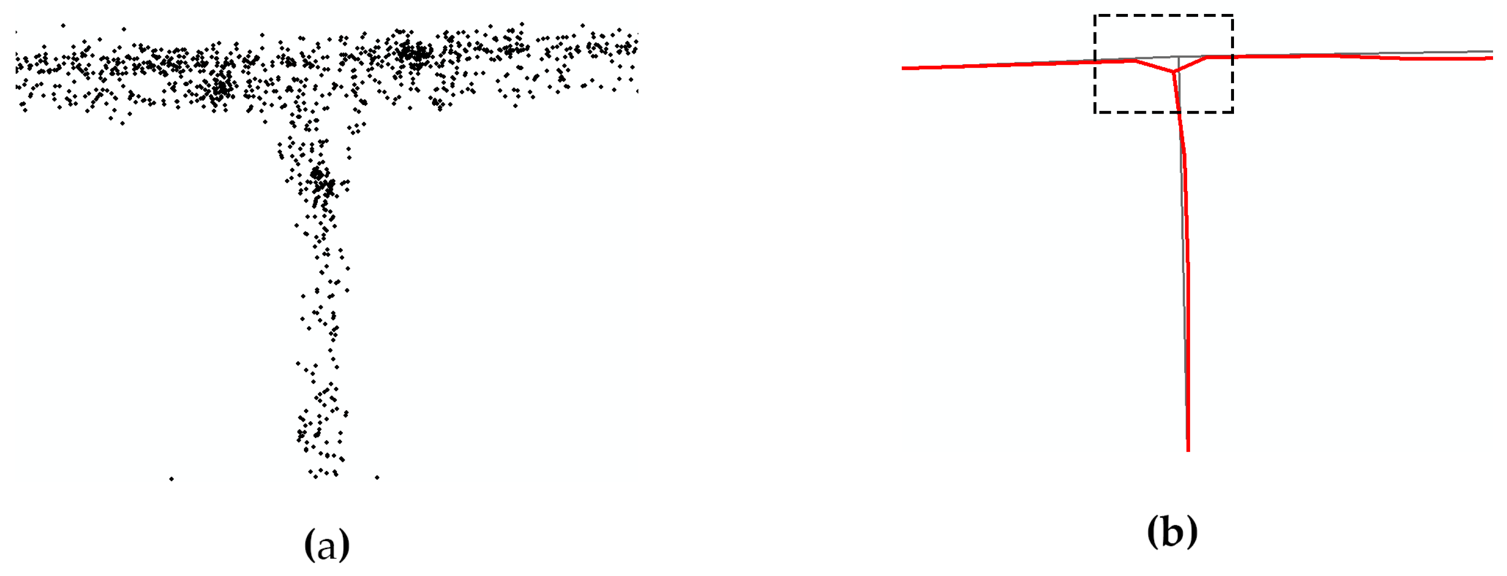
• For the third situation, which is illustrated in Figure 7d, before merging the sub-intersections, outliers and noise must be removed (Section 3.1.2 states that a road segment cannot cross through the intersection area where feature points have a smaller linearity value; thus, the sub-intersection defined by the intersection of road segment $l_2$ and the dashed line in Figure 6d is discarded). Hierarchical clustering [39] is then performed to calculate the remaining intersections (sets of data are grouped by maximizing the similarity among similar clusters and minimizing the similarity between different clusters), and the centroids of the clusters are then used as the intersections. As illustrated in Figure 7d, the remaining two sub-intersections, $k_1$ and $k_2$, are autonomous fragmented parts that preserve an irregular intersection because they are divided into two clusters.

Based on the merge and intersect strategy, the disconnected road segments extracted based on the previous step are checked and further connected one by one. Fathi [17] used 40 m to determine the coverage of intersections, which was 1.5 times the road skeleton search threshold used in this step to search for the endpoints of the road segment around the intersection. For example, as road $l$ is checked, the head nodes of road $l$ and other surrounding road segments within the threshold distance (head and tail nodes of nearby segments should be included) are found, and the road intersection is then extracted utilizing the above strategy. The same process is used to check and connect the tail node of road $l$, and a new road is then generated that maintains the topological features of the nearby road segments. The next road is modified in the same way until all the roads are checked. In this process, intersections are extracted based on the road segments extracted from the GNSS trajectories. More intersection confluence scenes are shown in Figure 8.

4. Experiments and Discussion

4.1. Datasets

To test the feasibility and effectiveness of the proposed intersection extraction method, two types of trace point datasets were used, and the features are described as follows. (1) The Chicago Campus Bus Dataset contains 118,364 GPS points and 889 trajectories within a region of 3.8 km × 2.4 km at the University of Illinois at Chicago [40], as shown in Figure 9a. Since the campus buses travel on relatively fixed routes, the GPS tracks are distributed over fixed roads and relatively clean. The dataset has been widely used in existing related work to evaluate map construction algorithms; (2) the Chengdu Taxi dataset was collected by taxis in the city of Chengdu, Sichuan, China, over an approximate duration of 1 day. The dataset covers a region of 3.4 km × 2.6 km, contains 2371 trajectories and approximately 501,861 points, and has a sampling rate that varies from 1 to 232 s. The taxi routes were not fixed shuttle in an urban region with a mixture of highways, high and medium volume roads, therefore, the track points are unevenly distributed on different volume roads with a lot of noise as shown in Figure 9b.

4.2. Evaluation Method

Road networks are important geographic entities that are presented in the form of complex networks, and they require high position precision and accurate topological relationships. The proposed method reconstructs intersections using extracted road segments, thereby improving the accuracy of the intersections and maintaining the morphologies of the road confluences. In this work, because the GNSS track points presented accuracy limitations, the real intersections were not all detected, and spurious intersections not present in the real word were found. An efficient intersection detection method should be able to detect a maximum number of ground truth intersections and minimize the number of spurious and missing intersections. Biagioni and Eriksson proposed a point-matching approach to measuring the accuracy of points based on three criteria: precision, recall, and F-measure [41]. The approach considered a one-to-one match between two groups of points (i.e., the extracted intersections and the truth intersections) at a given distance threshold and counted matching points between the two groups. The number of matched points increases quickly with increases in the distance threshold, and a smaller discrepancy between two groups corresponds to a faster period required to reach stability with a smaller distance threshold. Therefore, the accuracies of the intersections with respect to the ground truth map were quantified by the proportion of matched points, where the number of matched extracted intersections is represented by Matched-extracted, the number of matched truth intersections is represented by Matched-truth, the accuracy of the extracted intersection geometry is represented by precision, and the completeness of the number of extracted intersections is represented by recall, with $precision=Matched\_extracted/extracted$ and $recall=Matched\_truth/truth.$ To produce a composite performance index from these two values, the F-measure is defined as

$$F-measure=2\ast \frac{precision\ast recall}{precision+recall}$$

The F-measure ranges from 0 to 1, and scores close to 1 indicate that the extracted intersections performed better at position accuracy and completeness. In this work, this evaluation method was used to evaluate the geometric and completeness accuracies of the exacted intersections compared with that of a ground truth map.

4.3. Comparison and Discussion

Based on the experimental tests, the radius of the neighbourhood in the trajectory contraction was 30 m, and the thresholds for the segment growth process were 15° and a distance of 30 m. For comparison and evaluation, the road inference methods of Davies [22] and Ahmed [18] were used to extract intersections from the same datasets. These two open source algorithms are implemented in Python and Java and retain the original default parameter settings over the experiments. To measure the accuracy of the intersections extracted from the GPS traces, OpenStreetMap [42] was selected as the ground truth map for this work. To perform a qualitative evaluation of the results, the extracted intersections (highlighted points) were overlaid on the ground truth vector maps of the corresponding area as shown in Figure 8 and Figure 9.

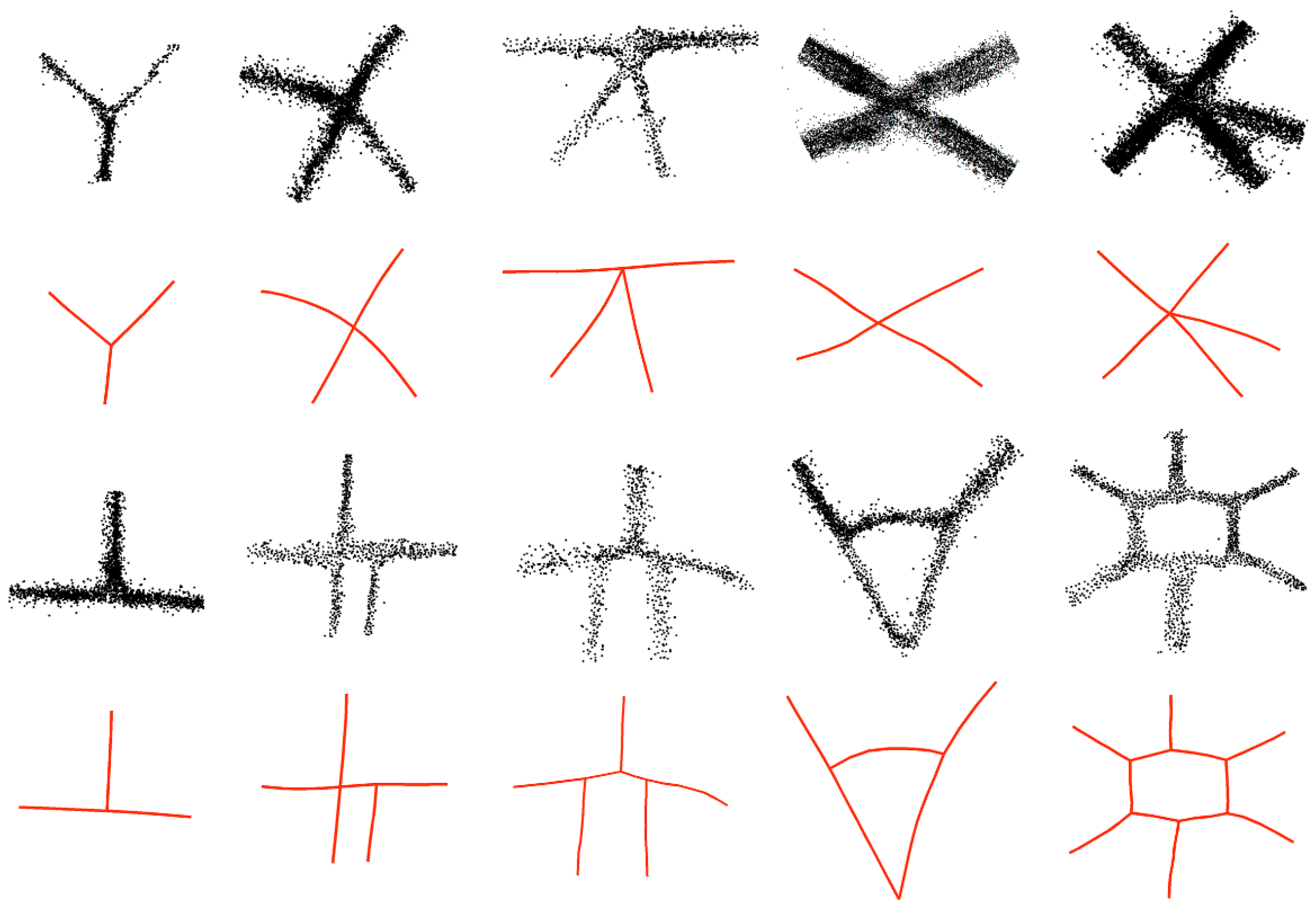
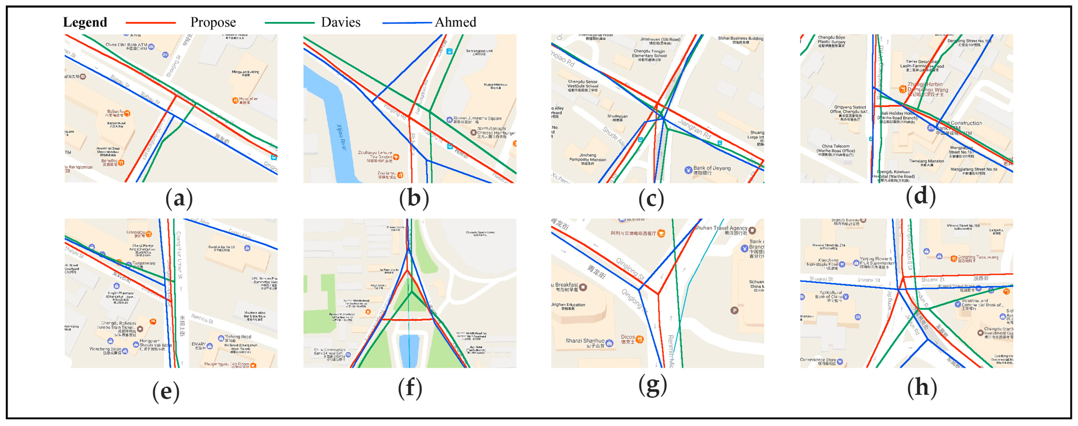
4.3.1. Visual Inspection

In Figure 10 and Figure 11, the extracted intersections are superimposed on the corresponding areas of the vector map to qualitatively evaluate the results. Figure 12 shows the detailed intersection results, which are compared with another method employing the Chengdu dataset. The visualization clearly shows that the proposed method extracted more intersections and showed considerable consistency with the ground truth map. Although Ahmed’s method can extract more intersections, it produces a large number of offset outputs and is messy (i.e., an excessive number of topology points at intersections are not merged), as shown in Figure 12c,h. Based on the positions and morphologies of the intersections, the proposed method was able to adapt to a variety of road intersections and was also able to extract the intersections with high precision; moreover, the orientations of the roads involved in constructing the intersections better conformed to the ground truth map.

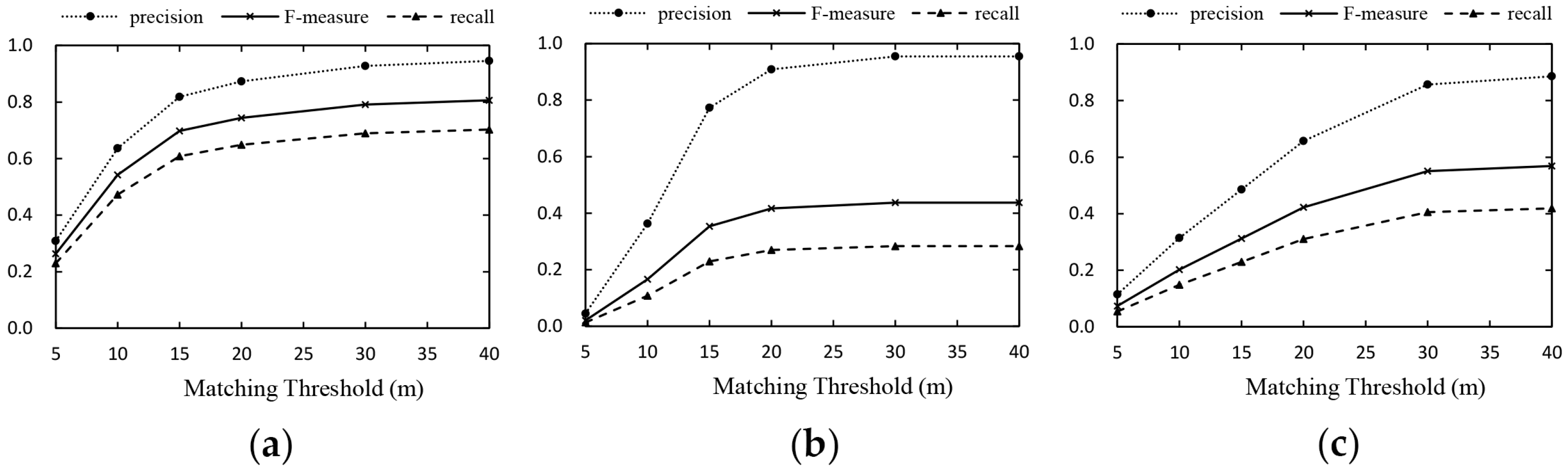
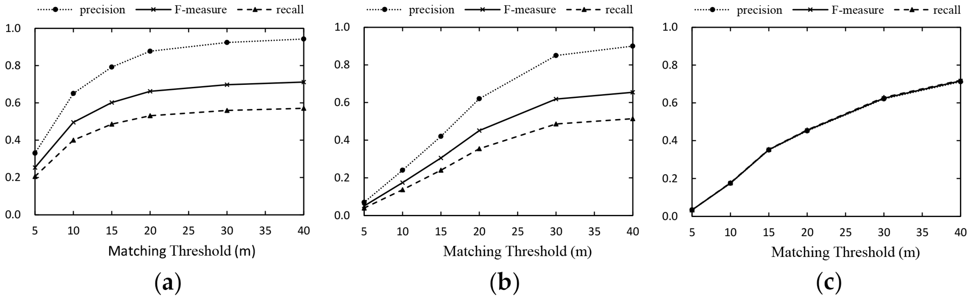
4.3.2. Accuracy Results

Table 1. Matched intersections with the threshold distance by the different methods.

Area	Method	Extracted/Truth 1	Number of Matched Intersections with the Threshold Distance (m)
			5	10	15	20	30	40	50
Chicago	Proposed	55/74	17	35	45	48	51	52	52
	Davies	28/74	1	8	17	20	21	21	21
	Ahmed	38/74	4	11	17	23	30	31	31
Chengdu	Proposed	106/175	35	69	84	93	98	100	102
	Davies	100/175	7	24	42	62	85	90	92
	Ahmed	177/175	6	31	62	80	110	126	138

¹ Extracted represents the number of intersections that are extracted, and Truth represents the number of real intersections.

lists the statistical results for the number of matched extracted intersections for different threshold distances in the two experimental areas. Based on the statistical results in Table 1, the position accuracies of the intersections detected from the two GPS trace point datasets using the additional models are compared in Figure 13 and Figure 14.

At matching distances of 5 m and 10 m, the number of matched intersections obtained by the proposed method was significantly better than that of the other two methods, especially for the lowest matching distance of 5 m. The results are listed in Table 1, and they indicate that the intersections extracted using the proposed method had higher position accuracies. Figure 13a and Figure 14a show that the criteria values of the proposed method increased as the matching distance threshold increased from 5 m to 20 m and increased slowly after the threshold reached 20 m. Figure 13b and Figure 14b demonstrate that the results from Davies’s method became constant after the matching distance thresholds reached 20 m and 30 m, respectively. The results obtained by Ahmed’s method for the Chicago stabilized at 30 m in Figure 13c, but the performance continued to increase with the Chengdu dataset as shown in Figure 14c. Therefore, the constant values of the curve indicate that the position offset of the intersections extracted using the proposed method were distributed over a small distance. For the Chengdu Taxi dataset, although Ahmed’s method matched more intersections than the proposed method in the range of 30 to 50 m, the intersections matched by Ahmed’s method are considered messy or spurious as shown in Figure 12c,h. These evaluation results indicate that the intersections extracted using the method proposed in this work had a higher accuracy in terms of geometry and were better able to preserve the morphology of the roads at the intersections.

5. Conclusions

A method for extracting intersections is proposed in this study. The method consists of two steps that rely solely on the locations of track points, and this method performs better in geometric accuracy and confluence morphology than the other two methods, especially for irregular junctions. First, a clustering algorithm is employed that uses the coordinates of the trajectory points. The decentralized trajectories are contracted at the midlines of the roads via the regularized mean-shift method, and a PCA and depth-first strategy are used to search the roads to avoid constructing short segments and ensure correct road morphologies. To identify the independent dominant orientations of an intersection, the degree of collinearity Cost measure, which is based on parallelism and compactness, is used to merge the approximately collinear road segments and detect the intersections along independent dominant orientations using intersecting lines to accurately determine the geometry of the confluences of the roads. The experiments indicate that the proposed method has improved accuracy based on the geometry and road orientations of intersections, especially for T-shaped road intersections.

However, the proposed method could not extract all the intersections because road segment extraction depends on a certain density of GNSS trace points. Extracting road centrelines from sparse trajectories is difficult. In addition, the appropriate coverage radius for intersections and collinear parameter thresholds are important when extracting intersections. In this study, these parameters were set according to experience or statistical analyses and were not explored in detail; thus, these would orient our future study.

References

1. Guo, T.; Iwamura, K.; Koga, M. Towards high accuracy road maps generation from massive GPS traces data. In Proceedings of the 2007 IEEE International Geoscience and Remote Sensing Symposium, Barcelona, Spain, 23–28 July 2007; pp. 667–670. [Google Scholar]
2. Wang, Y.; Liu, X.; Wei, H.; Forman, G.; Chen, C.; Zhu, Y. Crowdatlas: Self-updating maps for cloud and personal use. In Proceedings of the International Conference on Mobile Systems, Applications, and Services, Taipei, Taiwan, 25–28 June 2013; pp. 27–40. [Google Scholar]
3. Matisziw, T.; Demir, E. Inferring network paths from point observations. Int. J. Geogr. Inf. Sci. 2012, 26, 1–18. [Google Scholar] [CrossRef]
4. Li, L.; Xing, X.; Xia, H.; Huang, X. Entropy-weighted instance matching between different sourcing points of interest. Entropy 2016, 18, 45. [Google Scholar] [CrossRef]
5. Tong, X.; Liang, D.; Xu, G.; Zhang, S. Positional accuracy improvement: A comparative study in shanghai, china. Int. J. Geogr. Inf. Sci. 2011, 25, 1147–1171. [Google Scholar] [CrossRef]
6. Nagai, Y.; Itoh, M.; Inagaki, T. Adaptive driving support via monitoring of driver behavior and traffic conditions. Trans. Soc. Automot. Eng. Jpn. 2008, 39, 393–398. [Google Scholar]
7. Ahmed, M.; Karagiorgou, S.; Pfoser, D.; Wenk, C. A comparison and evaluation of map construction algorithms using vehicle tracking data. Geoinformatica 2014, 19, 601–632. [Google Scholar] [CrossRef]
8. Yang, B.; Zhang, Y.; Lu, F. Geometric-based approach for integrating VGI POIs and road networks. Int. J. Geogr. Inf. Sci. 2014, 28, 126–147. [Google Scholar] [CrossRef]
9. Zheng, Y.; Zhang, L.; Xie, X.; Ma, W.Y. Mining interesting locations and travel sequences from GPS trajectories. In Proceedings of the International Conference on World Wide Web, Madrid, Spain, 20–24 April 2009; pp. 791–800. [Google Scholar]
10. You, Q.; Krumm, J. Transit Tomography Using Probabilistic Time Geography: Planning Routes without a Road Map. J. Locat. Based Serv. 2014, 12, 211–228. [Google Scholar] [CrossRef]
11. Herrera, J.C.; Work, D.B.; Herring, R.; Ban, X.; Jacobson, Q.; Bayen, A.M. Evaluation of traffic data obtained via GPS-enabled mobile phones: The mobile century field experiment. Transp. Res. Part C Emerg. Technol. 2010, 18, 568–583. [Google Scholar] [CrossRef]
12. Das, S.; Mirnalinee, T.T.; Varghese, K. Use of salient features for the design of a multistage framework to extract roads from high-resolution multispectral satellite images. IEEE Trans. Geosci. Remote Sens. 2011, 49, 3906–3931. [Google Scholar] [CrossRef]
13. Unsalan, C.; Sirmacek, B. Road network detection using probabilistic and graph theoretical methods. IEEE Trans. Geosci. Remote Sens. 2012, 50, 4441–4453. [Google Scholar] [CrossRef]
14. Boichis, N.; Viglino, J.M.; Cocquerez, J.P. Knowledge based system for the automatic extraction of road intersections from aerial images. Int. Arch. Photogramm. Remote Sens. 2000, XXXIII, 27–34. [Google Scholar]
15. Hu, J.; Razdan, A.; Femiani, J.C.; Cui, M.; Wonka, P. Road network extraction and intersection detection from aerial images by tracking road footprints. IEEE Trans. Geosci. Remote Sens. 2007, 45, 4144–4157. [Google Scholar] [CrossRef]
16. Efentakis, A.; Brakatsoulas, S.; Grivas, N.; Lamprianidis, G.; Patroumpas, K.; Pfoser, D. Towards a flexible and scalable fleet management service. In Proceedings of the Sixth ACM SIGSPATIAL International Workshop on Computational Transportation Science, Orlando, FL, USA, 5–8 November 2013; pp. 79–84. [Google Scholar]
17. Fathi, A.; Krumm, J. Detecting road intersections from GPS traces. In Geographic Information Science: 6th International Conference, Giscience 2010, Zurich, Switzerland, September 14–17, 2010, Proceedings; Fabrikant, S.I., Reichenbacher, T., van Kreveld, M., Schlieder, C., Eds.; Springer: Berlin/Heidelberg, Germany, 2010; pp. 56–69. [Google Scholar]
18. Ahmed, M.; Wenk, C. Constructing street networks from GPS trajectories. In Proceedings of the European Conference on Algorithms, Ljubljana, Slovenia, 10–12 September 2012; pp. 60–71. [Google Scholar]
19. Wu, J.; Zhu, Y.; Tao, K.; Wang, L. Detecting road intersections from coarse-gained GPS traces based on clustering. J. Comput. 2013, 8, 2959–2965. [Google Scholar] [CrossRef]
20. Xie, X.; Bingyungwong, K.; Aghajan, H.; Veelaert, P.; Philips, W. Inferring directed road networks from GPS traces by track alignment. ISPRS Int. J. Geo-Inf. 2015, 4, 2446–2471. [Google Scholar] [CrossRef] [Green Version]
21. Wang, J.; Wang, C.; Song, X.; Raghavan, V. Automatic intersection and traffic rule detection by mining motor-vehicle GPS trajectories. Comput. Environ. Urban Syst. 2017, 64, 19–29. [Google Scholar] [CrossRef]
22. Davies, J.J.; Beresford, A.R.; Hopper, A. Scalable, distributed, real-time map generation. Pervasive Comput. IEEE 2006, 5, 47–54. [Google Scholar] [CrossRef]
23. Xie, X.; Liao, W.; Aghajan, H.; Veelaert, P.; Philips, W. Detecting road intersections from GPS traces using longest common subsequence algorithm. ISPRS Int. J. Geo-Inf. 2017, 6, 1. [Google Scholar] [CrossRef]
24. Tang, L.; Ren, C.; Liu, Z.; Li, Q. A road map refinement method using delaunay triangulation for big trace data. ISPRS Int. J. Geo-Inf. 2017, 6, 45. [Google Scholar] [CrossRef]
25. Chiang, Y.Y.; Knoblock, C.A. Automatic extraction of road intersection position, connectivity, and orientations from raster maps. In Proceedings of the ACM Sigspatial International Symposium on Advances in Geographic Information Systems, ACM-GIS 2008, Irvine, CA, USA, 5–7 November 2008; p. 22. [Google Scholar]
26. Shi, J.; Malik, J. Normalized cuts and image segmentation. IEEE Trans. Pattern Anal. Mach. Intell. 2002, 22, 888–905. [Google Scholar]
27. Ester, M.; Kriegel, H.P.; Xu, X. A density-based algorithm for discovering clusters a density-based algorithm for discovering clusters in large spatial databases with nois. In Proceedings of the International Conference on Knowledge Discovery and Data Mining, Portland, OR, USA, 2–4 August 1996; pp. 226–231. [Google Scholar]
28. Comaniciu, D.; Meer, P. Mean shift: A robust approach toward feature space analysis. IEEE Trans. Pattern Anal. Mach. Intell. 2002, 24, 603–619. [Google Scholar] [CrossRef]
29. Cheng, Y. Mean shift, mode seeking, and clustering. IEEE Trans. Pattern Anal. Mach. Intell. 1995, 17, 790–799. [Google Scholar] [CrossRef]
30. Qiu, J.; Wang, R. Automatic extraction of road networks from GPS traces. Photogramm. Eng. Remote Sens. 2016, 82, 593–604. [Google Scholar] [CrossRef]
31. Wang, J.; Yu, Z.; Zhang, W.; Wei, M.; Tan, C.; Dai, N.; Zhang, X. Robust reconstruction of 2d curves from scattered noisy point data. Comput.-Aided Des. 2014, 50, 27–40. [Google Scholar] [CrossRef]
32. Funke, S.; Ramos, E.A. Reconstructing a collection of curves with corners and endpoints. In Proceedings of the Twelfth Acm-Siam Symposium on Discrete Algorithms, Washington, DC, USA, 7–9 January 2001; pp. 344–353. [Google Scholar]
33. Koutaki, G.; Uchimura, K.; Hu, Z. Road Updating from High Resolution Aerial Imagery Using Road Intersection Model. Available online: http://www.isprs.org/proceedings/xxxvi/5-w1/papers/25.pdf (accessed on 9 December 2017).
34. Zourlidou, S.; Sester, M. Intersection detection based on qualitative spatial reasoning on stopping point clusters. ISPRS—Int. Arch. Photogramm. Remote Sens. Spat. Inf. Sci. 2016, XLI-B2, 269–276. [Google Scholar]
35. Luan, X.; Fan, H.; Yang, B.; Li, Q. Arterial roads extraction in urban road networksbased on shape analysis. Geomat. Inf. Sci. Wuhan Univ. 2014, 39, 327–331. [Google Scholar]
36. Regnauld, N. Généralisation du Bâti: Structure Spatiale de Type Graphe et Représentation Cartographique. Ph.D. Thesis, Provence University, Marseille, France, 1998. [Google Scholar]
37. Campbell, J. Map Use and Analysis, 4th ed.; McGraw Hill: Boston, MA, USA, 2001; ISBN 0-073-03748-6. [Google Scholar]
38. Touya, G. A road network selection process based on data enrichment and structure detection. Trans. GIS 2010, 14, 595–614. [Google Scholar] [CrossRef]
39. Karypis, G.; Han, E.H.; Kumar, V. Chameleon: Hierarchical clustering using dynamic modeling. Computer 2002, 32, 68–75. [Google Scholar] [CrossRef]
40. Biagioni, J.; Eriksson, J. Map inference in the face of noise and disparity. In Proceedings of the 20th International Conference on Advances in Geographic Information Systems, Redondo Beach, CA, USA, 6–9 November 2012; pp. 79–88. [Google Scholar]
41. Biagioni, J.; Eriksson, J. Inferring road maps from global positioning system traces. Transp. Res. Rec. J. Transp. Res. Board 2012, 2291, 61–71. [Google Scholar] [CrossRef]
42. OpenStreetMap. Available online: Http://www.openstreetmap.org/ (accessed on 11 May 2017).
Figure 1. Iterative calculation process and calculation results; the source point is the same as in Figure 1; (a) Calculated results after one iteration; (b) results after five iterations; and (c) results after 20 iterations.
Ijgi 06 00403 g001
Figure 2. Process of road segment growth. The green dots are candidate points and linearly distributed. (a) Seed point (highlight point) with the largest distribution characteristics value; (b) trace along the dominant principal component analysis direction of the seed point; (c) trace along the direction opposite the dominant PCA direction of the seed point; and (d) merged search results in both directions.
Ijgi 06 00403 g002
Figure 3. The intersection position deviation and road segments around the intersection are distorted, which connect directly with the end nodes of the road around the T-intersection. (a) The original GNSS input points; (b) T-intersection directly connected by road centrelines.
Ijgi 06 00403 g003
Figure 4. Calculating the geometric relationships between the segments at the same intersection. (a) The two roads are spatially parallel and neither intersect nor merge; (b) The two segments with two distinct orientations; (c,d) The two approximately collinear disjointed roads with larger Cost values should be combined into a single road.
Ijgi 06 00403 g004
Figure 5. Identifying collinear road segments around the intersection. (a) Input GNSS trajectories around the intersection; (b) road segments extracted from the input GNSS trajectories; and (c) two segments are combined into a single segment, and the other two segments remain unchanged. The black segments represent road segments, and the bold black segments represent the end segments of the road segments.
Ijgi 06 00403 g005
Figure 6. Detecting the location of the intersection based on the intersect of segments with conflicting orientations. (a) Identifying the conflicting road segments around the intersection from the previous steps; (b) road segments intersecting at multiple points; and (c) calculating the intersection location based on multiple points.
Ijgi 06 00403 g006
Figure 7. Connecting multiple line segments around an intersection. (a) T-intersection detected by the single intersection of segments on two conflicting orientations; (b) three-forked road intersected in three conflicting orientations, with an acute small triangle formed by the intersection of the three roads and the centroid of the triangle representing the intersection of the three roads; (c) crossroad with two conflicting orientations intersecting at one point; and (d) irregular intersection with multiple orientations and multiple sub-intersections.
Ijgi 06 00403 g007
Figure 8. Additional intersection reconstructions for different scenes. The black dots represent the GNSS track point inputs, and the red lines represent the extracted roads for which the topological features are preserved. When an intersection has two or more dominant orientations, all the orientations of the intersection converge to the location of the intersection.
Ijgi 06 00403 g008
Figure 9. (a) GPS trajectory dataset for Chicago; and (b) GPS trajectory dataset for Chengdu.
Ijgi 06 00403 g009
Figure 10. Extracted intersections (highlighted points) and road network (red lines) overlapped with the ground truth map (grey line) of the Chicago dataset. (a) Intersections and road network extracted by the proposed method; (b) intersections and road network extracted using Davies’s method; and (c) intersections and road network extracted using Ahmed’s method.
Ijgi 06 00403 g010
Figure 11. Extracted intersections (highlighted points) and road network (red lines) overlapped with the ground truth map (grey line) of the Chengdu dataset. (a) Intersections and road network extracted by the proposed method; (b) intersections and road network extracted using Davies’s method; (c) and intersections and road network extracted using Ahmed’s method.
Ijgi 06 00403 g011
Figure 12. Comparisons of the detailed intersection results obtained by the various methods employing the Chengdu dataset. Figure (ah) correspond to i to viii in Figure 11a.
Ijgi 06 00403 g012
Figure 13. Accuracy analysis of intersections from the Chicago dataset. (a) Proposed method; (b) Davies’s method; and (c) Ahmed’s method.
Ijgi 06 00403 g013
Figure 14. Accuracy analysis of intersections from the Chengdu dataset. (a) Proposed method; (b) Davies’s method; and (c) Ahmed’s method. Because of the small difference between the number of extracted intersections and real intersections, the precision, recall and F-measure nearly overlap.
Ijgi 06 00403 g014