Mapping Comparison and Meteorological Correlation Analysis of the Air Quality Index in Mid-Eastern China

Abstract

With the continuous progress of human production and life, air quality has become the focus of attention. In this paper, Beijing, Tianjin, Hebei, Shanxi, Shandong and Henan provinces were taken as the study area, where there are 58 air quality monitoring stations from which daily and monthly data are obtained. Firstly, the temporal characteristics of the air quality index (AQI) are explored. Then, the spatial distribution of the AQI is mapped by the inverse distance weighted (IDW) method, the ordinary kriging (OK) method and the Bayesian maximum entropy (BME) method. Additionally, cross-validation is utilized to evaluate the mapping results of these methods with two indexes: mean absolute error and root mean square interpolation error. Furthermore, the correlation analysis of meteorological factors, including precipitation anomaly percentage, precipitation, mean wind speed, average temperature, average water vapor pressure and average relative humidity, potentially affecting the AQI was carried out on both daily and monthly scales. In the study area and period, AQI shows a clear periodicity, although overall, it has a downward trend. The peak of AQI appeared in November, December and January. BME interpolation has a higher accuracy than OK. IDW has the maximum error. Overall, the AQI of winter (November), spring (February) is much worse than summer (May) and autumn (August). Additionally, the air quality has improved during the study period. The most polluted areas of air quality are concentrated in Beijing, the southern part of Tianjin, the central-southern part of Hebei, the central-northern part of Henan and the western part of Shandong. The average wind speed and average relative humidity have real correlation with AQI. The effect of meteorological factors such as wind, precipitation and humidity on AQI is putative to have temporal lag to different extents. AQI of cities with poor air quality will fluctuate greater than that of others when weather changes and has higher correlation with meteorological factors.

1. Introduction

Nowadays, with the development of the social economy and the impact of human production and life, environmental problems are becoming more and more serious; urban air quality is getting worse and worse; and it is urgent to study and solve the problem of air quality [1,2]. We began to monitor air quality very early, for example surface ozone over Athens, Greece, for the period 1901–1940. Comparing the historical data with the recent data, we can see the trend of air quality in big cities. Furthermore, it is necessary to re-evaluate historical data with new tools in recent years [3]. From the long-term variations of the broadband direct and diffuse irradiances, as well as the ones of turbidity coefficients, the time evolution of the air quality for a longer period in the past can be drawn indirectly [4]. A previous study reported that the various spectral wave bands for clear days showed a pronounced decline in the period 1966–1990 for Athens, which was attributed to the increase of air pollution due to the continuous development of the city in this period [5]. Air pollution has a certain correlation with the occurrence of lung cancer and cardiovascular disease [6,7,8,9]. The plausible association between increased levels of solar ultraviolet radiation, air-pollution at the ground level and the development of ocular skin defects (for example, erythema, cataract, cornea, conjunctiva, eyelid and lens damage) is studied in [10,11]. Urban air pollution makes the ground ultraviolet radiation significantly reduced (up to 50%) [12].

In recent decades, the Chinese economy has made incremental progress thanks to the policy of reform and opening; whereas, in the meantime, the air quality problems have deteriorated rapidly all over the whole country because of the lack of the parallel high-tech guarantee and environmental protection, especially in northern regions of China, such as Beijing, Tianjin, Hebei and Shandong. The air quality report from Ministry of Environment Protection of the People’s Republic of China shows that for 13 prefecture level cities in Beijing, Tianjin and Hebei, their average air quality standard day ratio is 37.5%, which is 23% lower than the other 74 cities. To evaluate the air quality quantitatively, some indices are proposed. The more recently used one is called the air quality index (AQI). AQI is a dimensionless quantity. It is a substitute for the air pollution index after the second half of the year 2012. AQI is based on the comprehensive assessment of six pollutants: sulfur dioxide, nitrogen dioxide, PM10, PM2.5, ozone and carbon monoxide, as stipulated by the Chinese government’s Ambient Air Quality Standard (GB3095-2012); see [13]. The index is divided into six levels according to its value. The higher the index or level is, the worse the air pollution is.

The AQI has temporal and spatial characteristics and is highly correlated in time and space. Time series analysis is an important method to study the temporal characteristics of air quality, while spatial interpolation is a primary method for exploring its spatial patterns. Commonly-used spatial interpolation methods include: (1) the gradient descent algorithm; (2) inverse distance weight methods; (3) kriging methods; (4) smoothing trend functions; (5) the polynomial approximation method; and (6) the space spline pre-estimation method. Bayesian maximum entropy proposed in recent years has also been widely used; see [14]. Bao et al. analyzed the distribution characteristics of air quality in China in time and space and revealed the cyclical nature of air quality in the seasons and the correlation between precipitation, pressure and temperature of air quality. AQI in the south is lower than the north, in the vertical direction; it declines with elevation; and with the increase in height, the trend of change gradually slows down [15,16]. Zhang analyzed air quality in Urumqi by gray correlation analysis and identified several covariates, which are related to air quality: industrial pollution, urban greening level, urban heating, automobile exhaust pollution, etc.; see [17]. Ashraf interpolated daily meteorological data from 17 stations in Nebraska, Kansas and Colorado from 1989–1990 by the inverse distance squares method, the inverse distance method, ordinary kriging and co-kriging and ascertained that co-kriging is the best one of these methods according to the comparison of root mean square interpolation error (RMSIE) [18]. The existing methods of spatio-temporal interpolation and their existing problems are summarized, and an improved spatio-temporal interpolation method is proposed in [19].

The remainder of the paper is organized as follows. Firstly, the materials and methods used in this paper are explained in Section 2 and Section 3. Then, the analysis of temporal and spatial characteristics is carried out, and the results are shown and discussed in Section 4. Next, the relationship between AQI and meteorological conditions is presented in view of the potential impact of several main meteorological factors, precipitation, wind, temperature, water vapor pressure and relative humidity, in Section 5. Finally, conclusions are drawn in Section 6.

2. Materials

2.1. Study Area

The study area of this paper covers Beijing, Tianjin, Hebei, Shanxi, Henan and Shandong. This area covers a total area of 712,300 square kilometers, with a population of 330 million that accounts for 24.2% of the nation. According to the Statistical Yearbook 2014, the GDP in the study area amounts to 27.2% of the nation. In terms of the health report from the national institutions, such as CDC, cancer morbidity has had a rapid increase in recent years. Some research also confirmed the significant correlation between cardiovascular diseases and air quality [6,7,8,9].

The study area is the most severely polluted one in China. Though the status of air quality is slightly getting better in recent years, the average days exceeding the normal standard are still more than 170. In the study area, there are in total 1710 daytimes of heavy pollution or above, which accounts for 44.1% of the whole nation. With regard to the seasons when air pollution occurs, the most frequent occurrences of heavy pollution are from January–March and October–December. The study area suffered from several large-scale heavy pollution processes in Decembers, and the days with heavy or above in the study account for 36.8% of the nation, which is remarkably higher than other months. Given the reason that the area is one of the most polluted areas in the country, with a dense population, diversified economic development levels, varied weather and terrain, we selected this study area to analyze the temporal and spatial characteristics of AQI.

There are 1436 monitoring stations of air quality in total all over China from the Ministry of Environment Protection of the People’s Republic of China website. There are 58 monitoring sites in Beijing, Tianjin, Hebei, Shanxi, Henan and Shandong. The study area, its location in China and the monitoring stations to be used are shown in Figure 1.

2.2. Data

In this paper, the AQI data are downloaded from the Ministry of Environment Protection of the People’s Republic of China website.

AQI takes the maximum of the six IAQI (individual air quality index) values (SO₂, NO₂, PM10, PM2.5, O₃, CO). IAQI is calculated as follows:

$$IAQ{I}_i=\frac{IAQ{I}_{Hi}-IAQ{I}_{Li}}{B{P}_{Hi}-B{P}_{Li}}\left(C_i-B{P}_{Li}\right)+IAQ{I}_{Li}$$

(1)

where $IAQ{I}_i$ represents the individual air quality index of the i-th pollutant. $C_i$ is the concentration of the i-th pollutant. $B{P}_{Hi}\mathrm{and}B{P}_{Li}$ are the high and low values of the pollutant concentration limit closest to $C_i$. $IAQ{I}_{Hi}\mathrm{and}IAQ{I}_{Li}$ are the individual air quality indices corresponding to $B{P}_{Hi}\mathrm{and}B{P}_{Li}$. The values of $IAQ{I}_{Hi}, IAQ{I}_{Li}, B{P}_{Hi}, B{P}_{Li}$ reference the Chinese government’s Ambient Air Quality Standard (GB3095-2012).

The monitoring network is composed of 58 ground-based monitoring sites scattered around the entire study area (Figure 1). All of the monitoring sites are equipped with instruments for continuous real-time monitoring of several kinds of air pollutants, including PM2.5, PM10, CO, SO₂, O₃ and NO₂. (Although PM2.5 and PM10 update every 24 h). It can provide a great quantity of samples for all kinds of studies in the field of atmospheric pollutants. The monthly meteorological data come from the China Meteorological Data website. The monitoring network is composed of 23 ground-based monitoring sites scattered around the entire study area. These meteorological data are abstracted from the daily dataset of China Ground International Exchange Stations. The dataset is from 194 basic ground meteorological stations. Data items include: average air pressure, average air temperature, average water vapor pressure, mean relative humidity, average wind speed, evaporation, sunshine duration and precipitation. The time range of these data is from August 2014–May 2016. The coordinate system used for the location information of these stations is WGS84.

We found that some stations have missed part of the early monthly data, from August 2014–November 2014, and other stations are complete. We call the stations with missing data as the incomplete data stations; others are complete data stations. There are 43 complete data stations and 15 incomplete data stations (Figure 1). When we use the data before November 2014 to perform the spatial interpolation, we only use the data of complete data stations.

3. Methods

The main contents of the integration of multi-method used in this research are composed of four parts, data extraction, preprocessing, spatial interpolation and correlation analysis (Figure 2). We obtained daily AQI data from the website of the Ministry of Environment Protection of the People’s Republic of China. The monthly meteorological data are downloaded from the China Meteorological Data Service website. Then, the data are preprocessed by a customized Python program. The stations contained in the study area are screened out and their locations are geocoded with a base map of the study area. The monthly mean of each station is calculated according to the daily data. Next, three interpolation methods are used to map the AQI data, and the mapping accuracy is evaluated and compared to one another. Finally, a correlation analysis between AQI and several main meteorological factors is carried out. The flowchart of AQI analysis is shown in Figure 2.

3.1. Spatial Interpolation

As shown in Figure 2, we use three kinds of interpolation techniques to map the spatial distribution of AQI in the study area.

Inverse distance weighting: The basic idea of inverse distance weighting interpolation (IDW) is: suppose the weight of the influence of the known sample point on the predicted point is inversely proportional to the distance between the two points. The smaller the distance, the bigger the interpolation weight is. For a given prediction point, the sum of the weights of all known sample points adjacent to it is always 1 [20]. IDW is formulated as:

$$X=\frac{{\displaystyle \sum _{i=1}^n\frac{X_i}{d_i^p}}}{{\displaystyle \sum _{i=1}^n\frac{1}{d_i^p}}}$$

(2)

where X is the estimated value for a prediction point. $X_i$ is the value for the i-th known sample point. $d_i$ is the distance between the i-th known sample point and the prediction point. p is the power of weight. Its value is usually taken as 2, and the most selected range is [0.5, 3].

Kriging: Kriging methods play an important role in geostatistics. Its main idea is to give different weights to the grade of each sample point according to the difference of the spatial position of the known sample points and the correlation between the sample points. After the moving weighted average, the average grade of the central area is estimated. It is formulated as:

$$z^{\ast }\left(x_0\right)={\displaystyle \sum _{i=1}^n{\lambda }_{i}z\left(x_i\right)}$$

(3)

where $Z^{*}\left(x_0\right)$ is the spatial estimated value of the predicted point. $Z\left(x_i\right)$ is the known attribute value of the i-th sample point. $n$ is the total number of sample points. ${\lambda }_i$ is the weight coefficient of the corresponding sample point.

For ordinary kriging, at each sample point, the expected value of the random function is re-estimated, and the sliding data neighborhood used by ordinary kriging makes the algorithm as a whole nonstationary, but the mean and covariance corresponding to the change are stable [21].

The basic steps of ordinary kriging can be referred to [22].

Bayesian maximum entropy: Christakos (1990) established the Bayesian maximum entropy (BME) method. The BME method takes many types of data and different types of knowledge bases into spatial interpolation. These data and information are divided into general knowledge ($K_G$) and site-specific knowledge ($K_S$) [23,24,25,26,27]. The Ks is composed of soft data and hard data. Hard data are the values obtained by measurement, while soft data are historical experience or data with high uncertainty. The steps for calculating BME include the prior stage, pre-posterior stage and posterior stage. In the prior stage, a maximum entropy theory as Equation (4) is used to obtain the prior distribution:

$$Inf{o}_G\left(Z_{map}\right)=-\log f_G\left(Z_{map}\right)$$

(4)

where $Z_{map}$ is the stochastic variable in the study area, $Z_{map}=\left(Z_{hard},Z_{soft},Z_0\right)$, and $Z_{hard}$, $Z_{soft}$ and $Z_0$ indicate the value of hard data, soft data and the location for estimating, respectively. $f_G\left(Z_{map}\right)$ indicates the pdf based on general knowledge $K_G$. Based on these constraints and the Lagrange multiplier approach, we can get the prior pdf:

$$f_G\left(Z_{map}\right)=A^{-1}\exp \left({\displaystyle \sum _{\alpha =1}^{N_c}{\mu }_{\alpha }{g}_{\alpha }\left(Z_{map}\right)}\right)$$

(5)

where ${\mu }_{\alpha }$ indicates Lagrange’s multiplier, $g_{\alpha }(Z_{map})$ is the known function associated with $Z_{map}$ based on $K_G$ and A indicates the normalization coefficient:

$$A={\displaystyle \int \exp \left({\displaystyle \sum _{\alpha =1}^{N_c}{\mu }_{\alpha }{g}_{\alpha }\left(Z_{map}\right)}\right)}d{Z}_{map}$$

(6)

In pre-posterior stage, the aim is to collect and organize additional auxiliary information in appropriate forms to produce site-specific knowledge. Then, they will be used in the BME model. Hard data have been incorporated into the prior stage indirectly and will be used directly at this stage.

In the posterior stage, a Bayesian conditionalization as Equation (7) is used to obtain the posterior distribution:

$$f_K\left(Z_0\right)=f_G\left(Z_0|Z_{hard},Z_{soft}\right)=f_G\left(Z_0,Z_{hard},Z_{soft}\right)\times {\left(f_G\left(Z_{hard},Z_{soft}\right)\right)}^{-1}$$

(7)

where $Z_{hard}=\left[x_1,...,x_n\right]\prime$, $Z_{soft}=\left[x_{n+1},...,x_m\right]\prime$ and n, m indicate the number of hard data and soft data within the scope of maximum distance $d_{\max }$ to the estimation point, respectively.

3.2. Spatial Autocorrelation

Semivariogram: Spatial autocorrelation plays an important role in geostatistics. Both the kriging and BME methods need considering spatial autocorrelation in their processes. French statistician Georges Matheron proposed the semivariogram as a quantitative measure of spatial autocorrelation in the 1960s [28].

The autocorrelation discussed in space is obviously related to spatial distance, and the function to measure this correlation is called the semivariogram [29], defined as:

$$r\left(h\right)=\frac{{\displaystyle \sum _{i=1}^{N\left(h\right)}{\left[a_i-a_{i+h}\right]}^2}}{2N\left(h\right)}$$

(8)

where r(h) represents the value of the semivariogram and N(h) represents the number of point pairs with distance h in the study area. The numerator represents the sum of the squares of the differences between the two attribute values of any two points with distance h. Generally, as the spatial distance h between two points increases, the correlation is getting smaller and smaller, which means the degree of variation is increasing. Therefore, the semivariogram increases slowly with the increase of spatial distance h [30]. The semivariogram can describe both the randomness and the structure of the regionalized variables better than other measures, such as spatial covariance [31].

Process of calculating semivariogram: We can estimate the semivariogram from the sample data. This estimated semivariogram is called the empirical semivariogram. For a study area, first calculate the distance between all of the point pairs. In this paper, there are 2415 pairs of points to be calculated; and find out the maximum and minimum values to determine lag distance h and lag level N. Starting from N = 1, find all point pairs $\left(P_i,P_j\right)$ that satisfied:

$$\left(N-1\right)h\le dis\left(P_i,P_j\right)\le Nh$$

(9)

The distance of the point pairs is denoted by $DI{S}_i$. Then, calculate the square of the difference between the attribute values.

$$S_i={\left[a\left(P_i\right)-a\left(P_j\right)\right]}^2$$

(10)

The number of point pairs we can find is $N\left(h\right)$. Calculate the average distance.

$$h_{avg}=\frac{1}{N\left(h\right)}{\displaystyle \sum _{i=1}^{N\left(h\right)}DI{S}_i}$$

(11)

The value of the semivariogram at this lag level is calculated by:

$$r^{\ast }\left(h_{avg}\right)=\frac{1}{2N\left(h\right)}{\displaystyle \sum _{i=1}^{N\left(h\right)}{S}_i}$$

(12)

Draw the points $\left(h_{avg},r^{*}\left(h_{avg}\right)\right)$ for each lag level and fit the points with a selected model. Thus, we get the empirical semivariogram. Several commonly-used models for fitting the semivariogram include the spherical model, the Gaussian model, the exponential model, etc. [32].

3.3. Cross-Validation

The cross-validation method is: First, the original sample data are divided into K different sets. Each time a K − 1 set is used as the training sample data, and the remaining group as the test data, calculate the relative error of the test data between the predicted and actual value after training. Each set is used only once as test data, repeated N times to ensure that the K sets of the data have been tested. The mean or root mean square of the error will be used for testing [33].

3.4. Interpolation Accuracy Evaluation

Two indices are used to evaluate the interpolation accuracy, one is mean absolute error (MAE), defined as:

$$MAE=\frac{{\displaystyle \sum _{i=1}^{m}abs\left(x_{a,i}-x_{e,i}\right)}}{m}$$

(13)

The other is root mean square interpolation error (RMSIE), defined as

$$RMSIE=\sqrt{\frac{{\displaystyle \sum _{i=1}^m{\left(x_{a,i}-x_{e,i}\right)}^2}}{m}}$$

(14)

where m represents the number of samples, $x_{a,i}$ represents the actual measured AQI for the i-th sample station and $x_{e,i}$ represents the estimated AQI by the spatial interpolation for the i-th sample station. Spatial interpolation of high precision has a small value of the two indicators. MAE is mainly used to evaluate the upper limit of error and the lower limit of error, but RMSIE is better at evaluating the sensitivity of spatial interpolation results and the maximal minimum effect of some sample points [34].

3.5. Temporal Correlation

For each station within the study area, the monthly meteorological data and AQI data can be viewed as two independent time series. We want to analyze the correlation between these two time series. The correlation of two time series can be expressed by the correlation coefficient, defined as:

$$r=\frac{n{\displaystyle \sum _{i=1}^n{x}_i{y}_i}-{\displaystyle \sum _{i=1}^n{x}_i}\times {\displaystyle \sum _{i=1}^n{y}_i}}{\sqrt{n{\displaystyle \sum _{i=1}^n{x}_i^2}-{\left({\displaystyle \sum _{i=1}^n{x}_i}\right)}^2}\times \sqrt{n{\displaystyle \sum _{i=1}^n{y}_i^2}-{\left({\displaystyle \sum _{i=1}^n{y}_i}\right)}^2}}$$

(15)

where x = {x₁, x₂, …, x_n} and y = {y₁, y₂, …, y_n} represent two different time series, r is in the range of [–1, 1]. R > 0 for positive correlation; r < 0 for negative correlation; r = 0 represents the absence of correlation. The greater the correlation, the higher the absolute value of r. It is generally believed that the absolute value of r is a micro correlation between 0 and 0.3, a real correlation between 0.3 and 0.5, a significant correlation between 0.5 and 0.8 and a high correlation between 0.8 and 1 [35].

4. Analysis of Temporal and Spatial Characteristics

We used each of the three interpolation methods to map the spatial distribution individually. The time span of the data duration includes 25 months from August 2014–August 2016. We selected nine months to demonstrate the analysis results. In the subsequent exhibition, the figure panels are read from left to right, from top to bottom: August 2014, November 2014, February 2015, May 2015, August 2015, November 2015, February 2016, May 2016, August 2016. Cross-validation is used to evaluate the accuracy of each interpolation method; every station is one set.

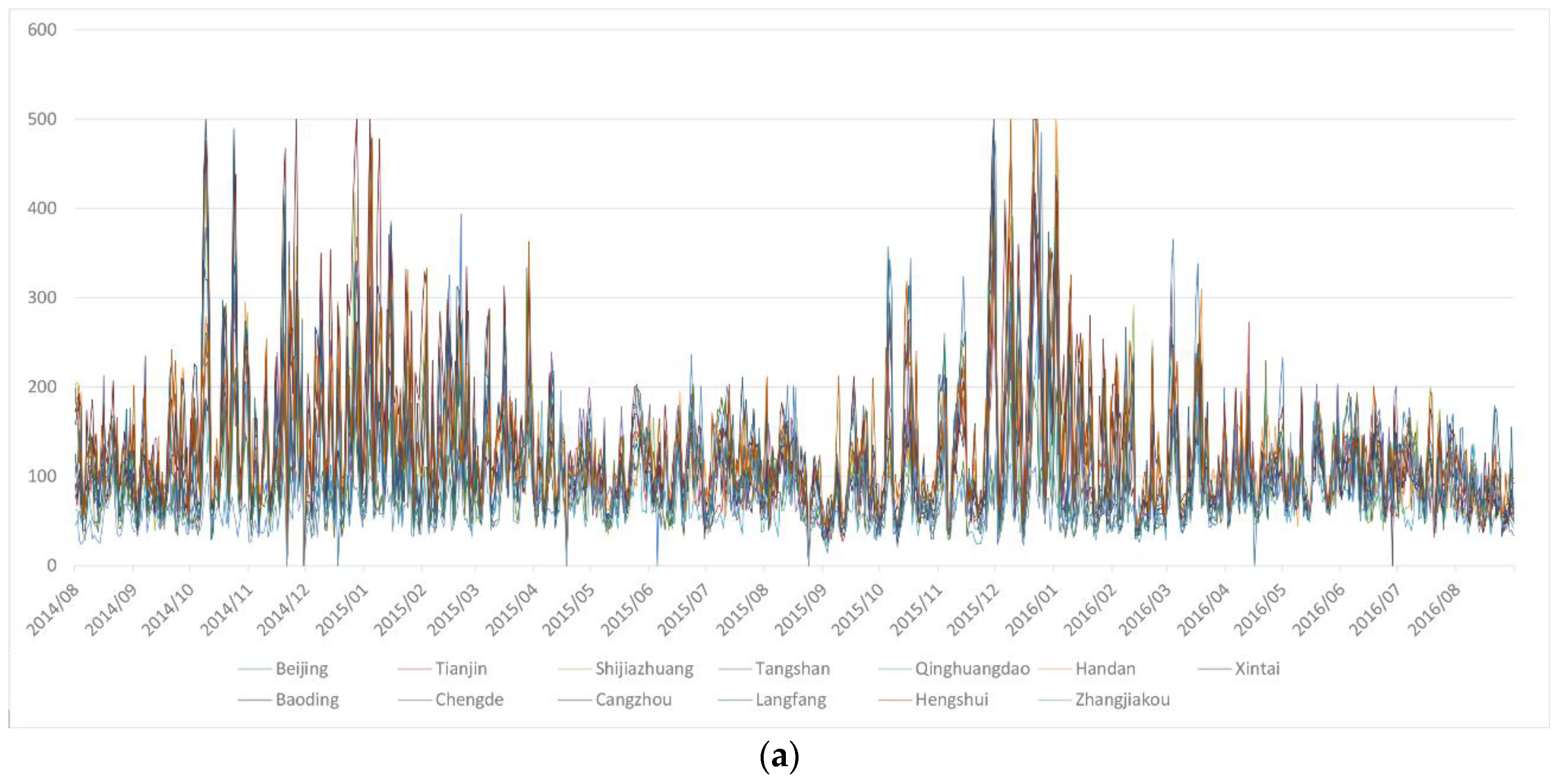
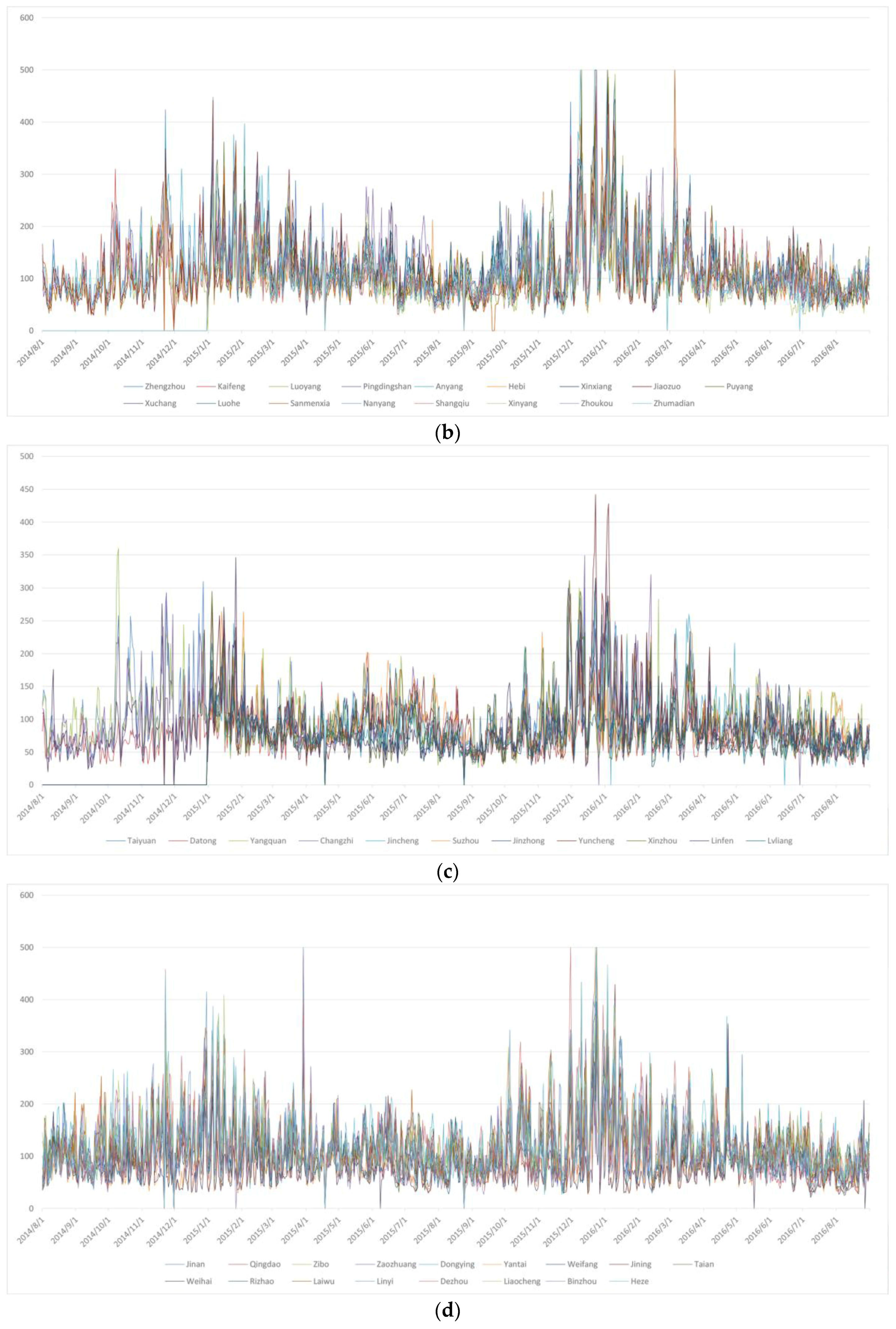
4.1. Temporal Characteristics

In order to study the trend and temporal characteristics of AQI, the AQI trend curves of all 58 stations and the annual AQI radar map were drawn. See Figure 3 and Figure 4.

We also calculated some significant statistical indicators based on the daily AQI data.

Table 1. Significant statistical indicators of the daily AQI data.

Station	Mean	Mean (2014)	Mean (2015)	Variance	Variance (2014)	Variance (2015)	Max	Min
Beijing	117.68	119.20	116.17	5457.34	4640.34	6275.74	485	23
Tianjin	104.38	108.90	99.89	3316.49	3228.31	3372.55	391	27
Baoding	145.85	160.73	131.10	7485.18	8055.78	6501.22	500	35
Yangquan	98.33	100.54	96.14	2083.73	1853.59	2308.03	360	26
Linfen	87.65	84.36	90.90	1964.32	1747.82	2163.05	346	20
Zhengzhou	129.78	134.62	124.98	4245.17	3755.58	4695.95	500	38

shows some of the results.

As seen from Figure 3, AQI shows a clear periodicity over time, and it is easy to see from Figure 4 that the peak of AQI appeared in November, December and January. From the trend curves and radar maps, one can see that in recent years, the total AQI showed a downward trend; the calculation results in Table 1 also support this conclusion. The calculation results show that AQI fluctuates more drastically over time, although it shows a downward trend.

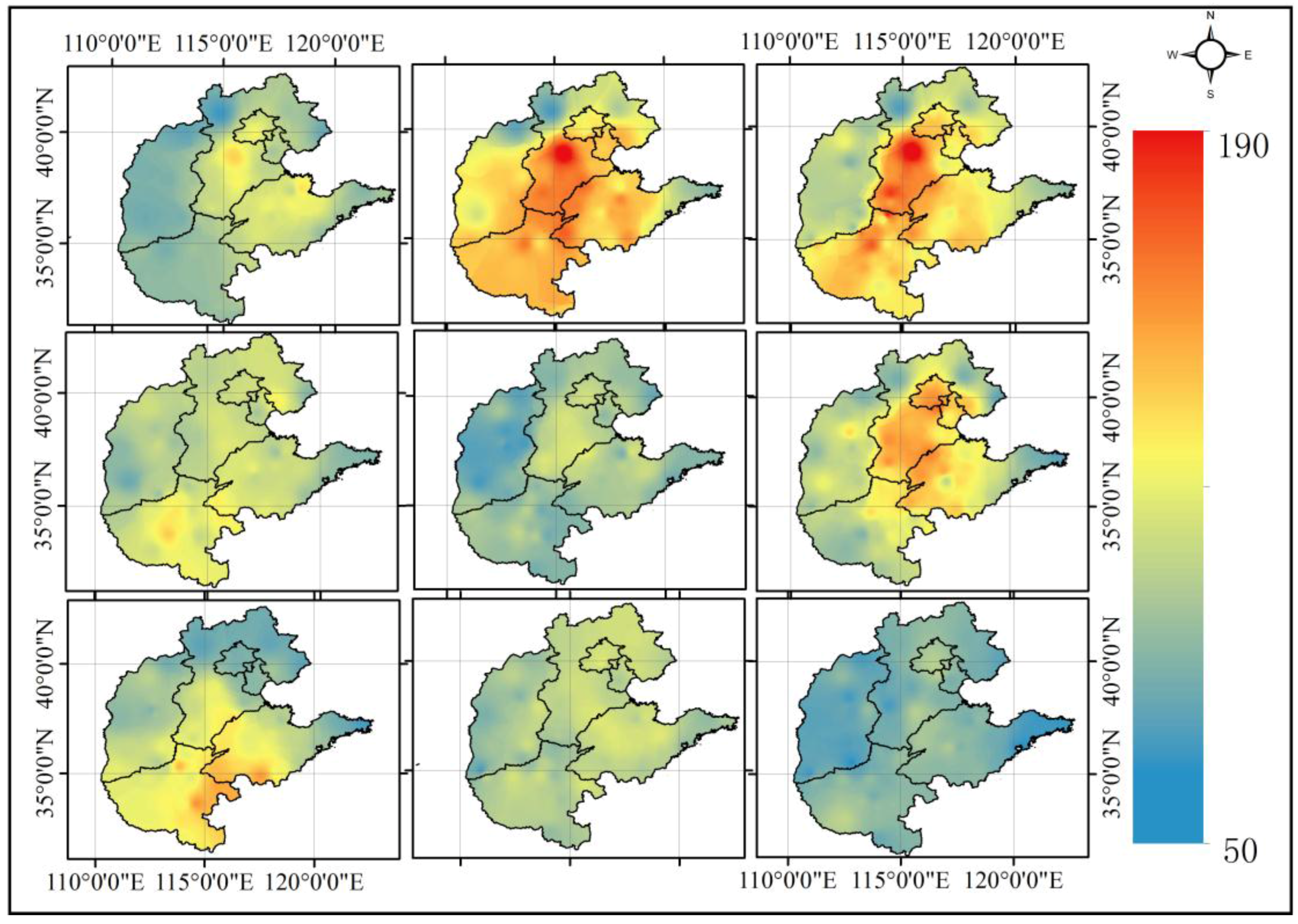
4.2. AQI Mapping with IDW

We use cross-validation results of 58 stations to select parameters. Considering that the search diameter should be less than half of the study area, we look for the optimal parameters in [2, 3.5]. Maximum and minimum adjacent feature is found in three combinations: [2, 5], [5, 10] and [10, 15]. The power exponent is found in three combinations: 1.5, 2 and 2.5. Results show that the search diameter has little effect on the interpolation results; a small adjacent feature leads to higher accuracy; and the power exponent leads a better result when set in 1.5 and two.

Finally, interpolation parameter settings with IDW are determined as follows: power exponent = 1.5, search radius = 2.69 (with a circle area), maximum adjacent feature = 10, minimum adjacent feature = 5. The results of IDW are shown in Figure 5.

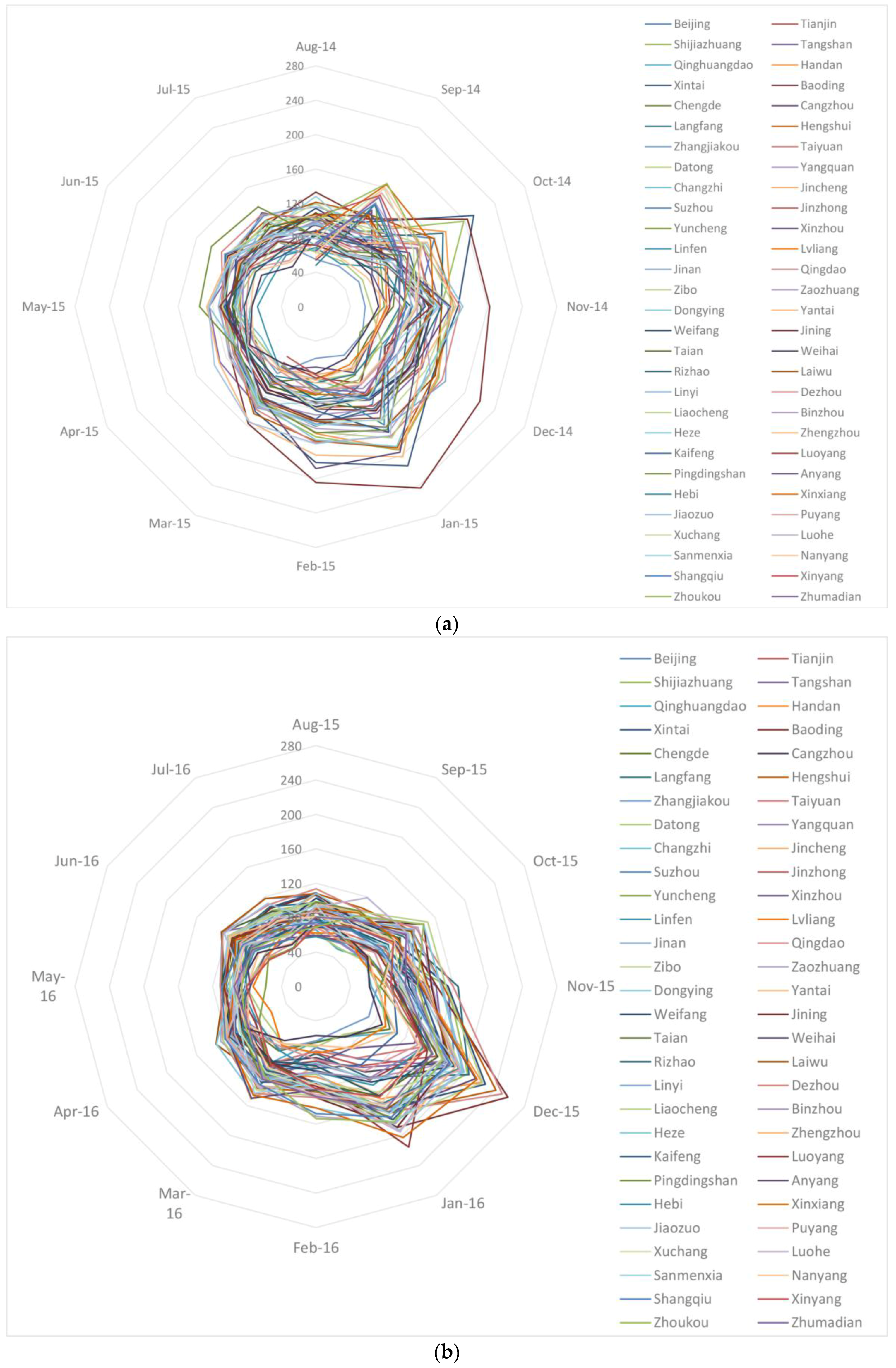
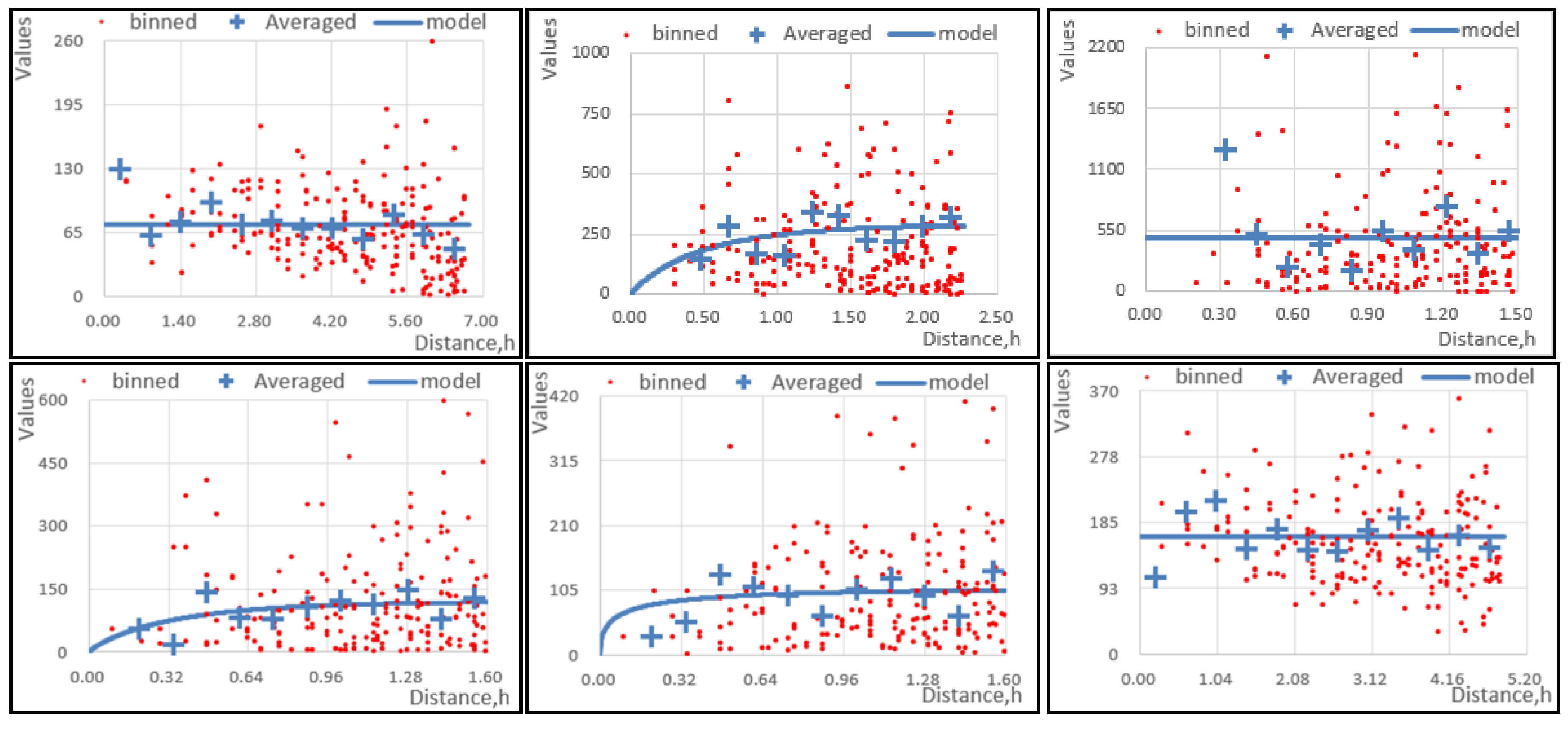
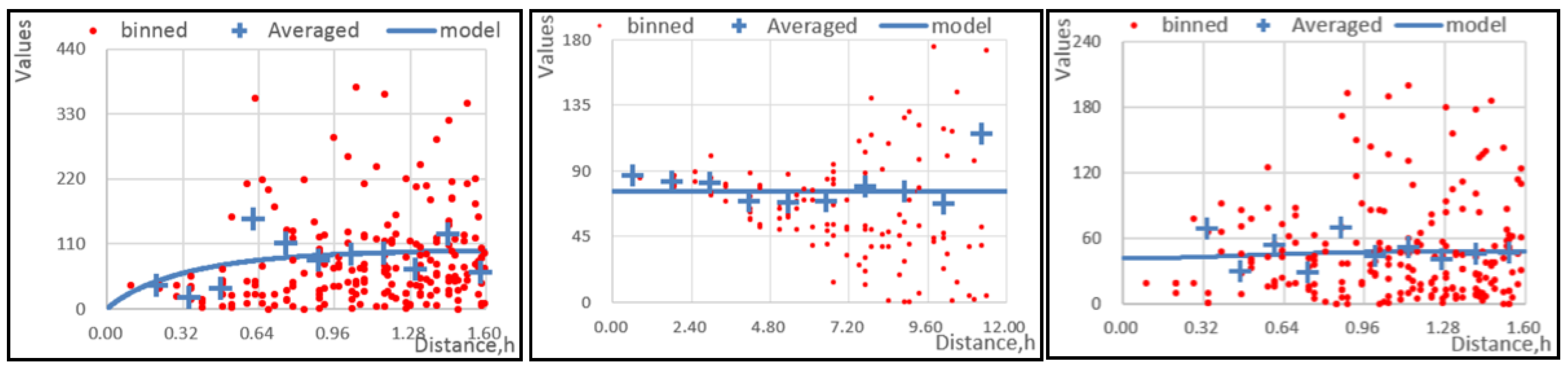
4.3. AQI Mapping with Kriging

We examine the distribution of the AQI data through several ESDA (exploratory spatial data analysis) techniques, such as histogram, quantile-quantile (Q-Q) diagram and 3D scatterplot, before kriging these data.

From Figure 6, we can see the AQI generally follows a normal distribution and has a second order of trend. After getting insights into the data, we select the exponential kernel function model to remove the trend of the data. Model parameter optimization uses an iterative cross-validation technique. The semivariogram is calculated after trend removal. We assume that the semivariogram is isotropic. Its parameters, nugget, partial sill and others, are optimized using cross-validation focusing on the estimation of these parameters.

The semivariogram is calculated by ArcGIS and then interpolated using the ordinary kriging method. The interpolated parameters of ordinary kriging are shown in

Table 2. Interpolation parameters of ordinary kriging.

Month	Nugget	Parameter	Major Range	Partial Sill	Lag Size
August 2014	72.562	0.2	4.5	0	0.56249
November 2014	0	0.91016	1.6529	290.05	0.18965
February 2015	486.36	0.2	1.0211	0	0.12764
May 2015	0	0.88027	1.1841	120.27	0.13472
August 2015	0	0.43906	1.1841	108.53	0.13474
November 2015	165.83	0.2	3.2688	0	0.40860
February 2016	0	0.90488	1.1841	100.52	0.13717
May 2016	75.69	0.2	14.213	0	1.18445
August 2016	42.136	2	1.1841	6.6152	0.13353

.

The minimum and maximum number of adjacent elements also need to be determined. We find when this number increases, the interpolation precision decreases slowly. Therefore, it is set to [2,3,4,5].

In the calculation of the semivariogram, the number of steps (lag level) is 12; the search field is a standard circle; the minimum number of adjacent elements is two; and the maximum is five. The search field (a circle) is divided into four sectors and deflected by 45°.

The stable model was used to fit the semivariogram function. The stable model is formulated as [22,36]:

$$\mathsf{\gamma }\left(h;\theta \right)={\theta }_s\left[1-exp\left(-3{\left(\frac{h}{A}\right)}^{{\theta }_e}\right)\right]$$

(16)

where ${\theta }_s$ represents the partial sill, h represents distance, A is the major range and ${\theta }_e$ is a parameter (Table 2). The complete semivariogram expression is:

$$\mathrm{Values}\left(h\right)={\theta }_0+\mathsf{\gamma }\left(h;\theta \right)$$

(17)

where ${\theta }_s$ represents the nugget. The semivariogram model for each month is drawn according to the interpolation parameters in Table 1, as shown in Figure 7. The results of ordinary kriging interpolation are shown in Figure 8.

4.4. AQI Mapping with BME

The spatial distribution of AQI is represented as a spatial random field. The purpose of the present work was to estimate the values of the random field at a non-measuring location by given data. We define complete data and incomplete data as hard data and soft data respectively in this paper.

See Figure 1; there are 15 incomplete data stations, and the probability density function of the air quality at these stations is calculated as the soft data. The probability density function of partial stations is shown in Figure 9.

The hard data are those measured AQI values. The semivariograms fitted in Section 4.3 are used to perform BME estimation. There are three key parameters that need be determined when mapping with BME: max number of hard data, max number of soft data, max search radius. After examining the process, we find including too much hard data and soft data will reduce accuracy; the larger search radius has little influence when the search field exceeds a certain limit. Finally, we set the max number of hard data = 5, soft data = 3 and radius = 2.69. Mapping results are shown in Figure 10.

4.5. Cross-Validation and Comparison

The cross-validation results are shown in

Table 3. Cross-validation result of three interpolation methods. OK, ordinary kriging; BME, Bayesian maximum entropy.

Time	Method	MAE	RMSIE	Time	Method	MAE	RMSIE
August 2014	IDW	11.2923	14.8369	November 2015	IDW	16.8145	21.3827
	OK	10.9151	14.1755		OK	13.3573	16.6038
	BME	9.4169	12.4072		BME	16.0600	20.0600
November 2014	IDW	17.8546	24.1299	February 2016	IDW	9.6880	12.2206
	OK	14.0996	18.6090		OK	8.9560	11.3090
	BME	17.6734	21.8362		BME	9.2500	11.5400
February 2015	IDW	20.0113	26.6201	May 2016	IDW	8.5534	10.8039
	OK	18.1584	24.6983		OK	8.9295	10.7937
	BME	17.7400	23.1100		BME	8.8525	11.0317
May 2015	IDW	9.2370	11.8869	August 2016	IDW	7.8679	9.6368
	OK	9.2512	11.8708		OK	7.7776	9.8154
	BME	8.8569	11.6275		BME	7.5564	9.6982
August 2015	IDW	9.8277	12.1164
	OK	9.9885	12.1584
	BME	9.5299	11.7899

. Figure 11 is the column comparison charts of the accuracy for three interpolation methods. The evaluation quantities used are MAE and RMSIE.

Comparing the air quality maps made by three interpolation methods, it can be found that there are obvious extreme points on the distribution map of the IDW method, while the other two methods make the distribution maps more flat.

As a deterministic local interpolation method, IDW only considers the spatial distance as the factor affecting the weight; the power exponent is fixed and chosen empirically, which makes the estimation of the unmeasured points very inaccurate; OK takes into account the spatial autocorrelation of AQI between the spatial points, but only calculates the semivariogram from known data locations and uses this single semivariogram in predicting the unknown points. This process implicitly assumes that the estimated semivariogram is the true semivariogram of the interpolation area. Since the uncertainty of semivariogram estimation is not taken into account, ordinary kriging underestimates the standard error of prediction. The Bayesian maximum entropy method takes into account the additional soft data, constructs the prior probabilities using the existing data and obtains more accurate interpolation results by calculating the posterior probability.

In theory, the accuracy of the BME method should be higher than OK, and OK is higher than IDW. The results of the actual evaluation also prove this to some extent. As shown in Figure 11, the accuracy of the three interpolation methods varies at different times, but in general, the BME method is the best; and OK is higher than IDW.

In a certain year, it can be seen that the AQI of winter (November) and spring (February) is much worse than summer (May) and autumn (August). The distribution of AQI has obvious spatial characteristics. The most polluted areas of air quality are concentrated in the central-southern part of Hebei and the central part of Henan, followed by Beijing, the southern part of Tianjin and the western part of Shandong. The air quality in Shanxi, the eastern and northern parts of Hebei and the eastern part of Shandong is relatively good.

The heavily-polluted areas are the densely-populated areas of Beijing, Tianjin, Hebei, Shandong and Henan, where large numbers of cities and factories are gathered, producing large amounts of pollutants. The wind speed in these areas is lower because of a large number of urban buildings, which makes contaminants not be easily spread. The air quality is better in areas with less population, where the city distribution is sparse and there is not so much heavy industry, producing fewer pollutants. The areas next to Inner Mongolia or near the sea have high wind speed. The generated contaminants will be blown away quickly. The air near the ocean has a higher air humidity and, so, a better air quality than the inland areas.

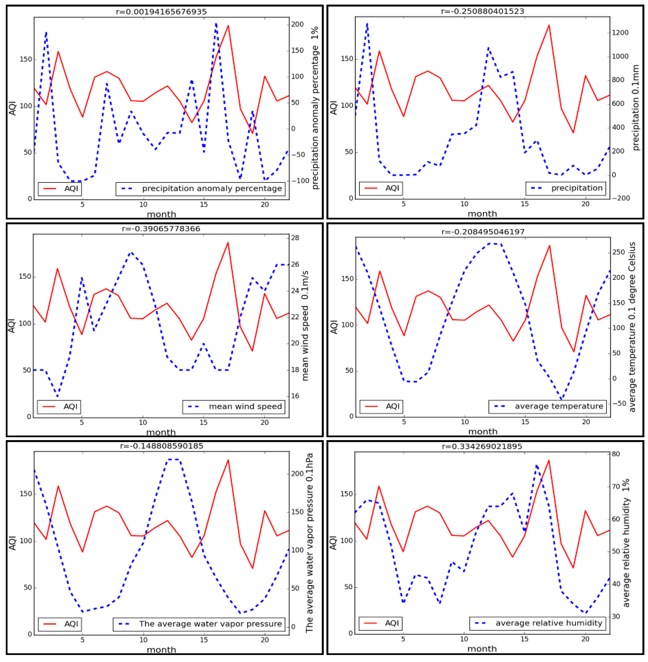
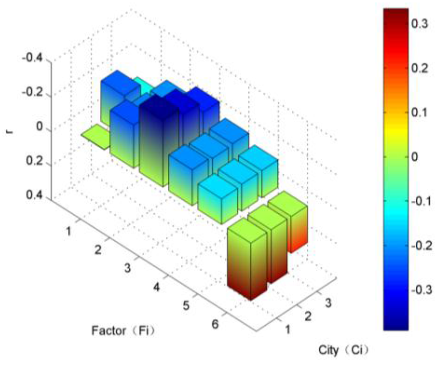
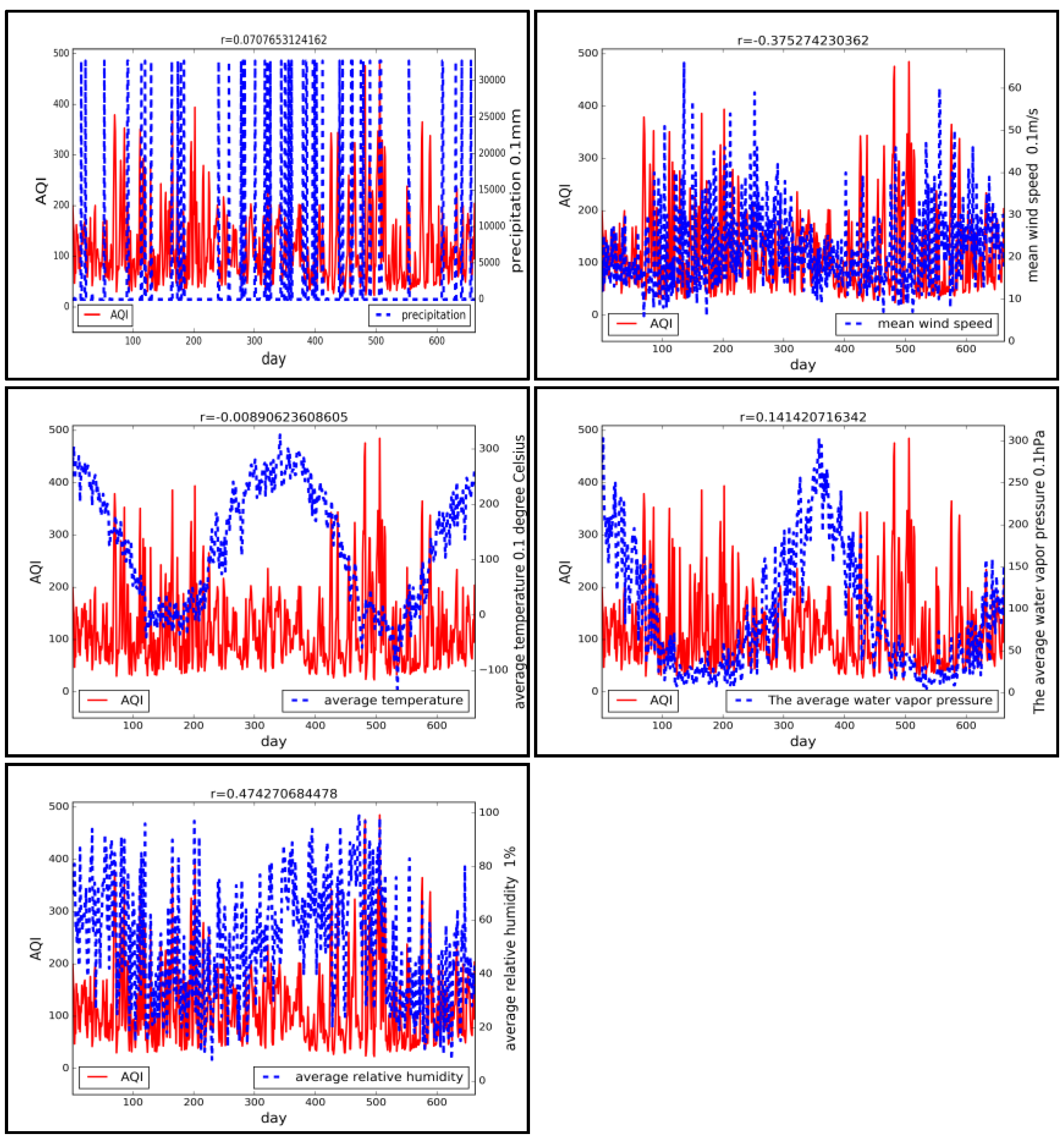
5. Relationship between AQI and Meteorological Conditions

The monthly meteorological data from August 2014–May 2016 of Beijing, Tianjin and Zhengzhou (the capital of Henan Province) are extracted based on the downloaded monthly data. These data include six meteorological factors: precipitation anomaly percentage, precipitation, mean wind speed, average temperature, average water vapor pressure, average relative humidity. The correlation between each factor and AQI was analyzed with the temporal correlation algorithm. The curves of time series and the correlation coefficients of the AQI with every meteorological factor are shown in Figure 12.

Figure 12 uses August 2014 as zero of the x-axis, showing the trend of the two time series in 22 months. r is the calculated correlation index.

In order to study the correlation between AQI and meteorological factors in different cities, the three-dimensional histogram of time series correlation of six factors in three cities was made; see Figure 13.

For comparison reasons, we analyzed the correlation between daily AQI and daily meteorological data from August 2014–May 2016 of Beijing, Tianjin and Zhengzhou. These data are obtained as described before in a daily scale. Five meteorological factors, precipitation, mean wind speed, average temperature, average water vapor pressure and average relative humidity, are involved in this analysis. The curves of time series and the correlation coefficients are shown in Figure 14 and Figure 15.

To investigate whether there is a delay in the correlation between meteorological factors and air quality, we made a cross-correlation analysis for the two daily time series. The results are shown in Figure 16.

From Figure 12 and Figure 13, it can be seen that the average wind speed and average relative humidity have a real correlation; there is a micro correlation in precipitation and average temperature; the other two factors have a small correlation; the mean wind speed is negatively correlated with AQI; and the relative humidity is positively correlated with AQI.

In Figure 14 and Figure 15, we use daily data to calculate the correlation coefficient. It can be found that the results are approximately the same as those calculated using monthly data, but have a larger variance. Only the average wind speed and average relative humidity have reached real correlation. The factors that have a high correlation coefficient calculated using monthly data will have a higher correlation coefficient than using daily data, while the low ones will have a lower value. There is reason to believe that by using daily data, we obtain a more accurate correlation.

From Figure 16, we can see that the lag effect of precipitation on AQI is from positive to negative. Additionally, the relative humidity has a positive correlation with AQI while considering temporal lag. We think the precipitation has an immediate effect of decreasing AQI and increases the air humidity subsequently, which leads to the effect of the increase on AQI indirectly. The wind has an immediate effect of decreasing AQI, which is consistent with our intuition because the wind can blow the polluted air away. High temperature seems to worsen the air quality, and the longer lag effect of temperature is obvious. Water vapor pressure has a negative lag effect on AQI.

The micro negative correlation between AQI and average temperature is corresponding with the mapping results in Section 4. The heating is supplied in the winter and spring in the study area, and there is a low absolute humidity, while the summer and autumn do not need heating; and there is a high absolute humidity. However, some existing studies also imply that the impact of heating on air quality is not as large as imagined. It may be because other industries output less pollutants in winter although the heating increased emissions of pollutants. As a result, the overall pollutants do not increase so much. The micro negative correlation between AQI and precipitation is easy to understand. Raindrops can take away the dust and particles in air, making it more difficult for haze to form. The real negative correlation between AQI and mean wind speed is because that wind will blow away pollutants. The average relative humidity is real positively related with AQI. Relative humidity means the ratio of absolute humidity to saturated humidity at the same temperature and air pressure. Although the absolute humidity is very low in winter and spring, the relative humidity is high. The correlation between relative humidity and AQI is the highest in the six factors. The trend of two series is consistent, as seen in Figure 11. It is possible to find factors that have a higher correlation and direct impact on AQI through the study of influence factors of the relative humidity further. Moreover, the correlation between six factors and AQI showed a consistent trend in three cities. This shows that the temporal correlation between AQI and these meteorological factors exists universally. There are also some differences between cities. The correlation between AQI and these meteorological factors in Beijing is greater than that in Tianjin and Zhengzhou. Combining the AQI distribution map in Section 4, we can find that AQI in a city with poor air quality will fluctuate greater than others when weather changes and has a higher correlation with meteorological factors.

6. Conclusions

In this paper, the mid-eastern China of Beijing, Tianjin, Hebei, Shanxi, Shandong and Henan provinces were taken as the study area. Then, the distribution of AQI was mapped by the inverse distance weighting method, the kriging method and the Bayesian maximum entropy method. The correlation between AQI and meteorological factors was analyzed by temporal correlation analysis. After discussing and analyzing the results, the following conclusions are drawn:

(1)

In recent years, AQI shows a clear periodicity, although overall, it has a downward trend. AQI fluctuates more drastically over time; the peak of AQI appeared in November, December and January.

(2)

Bayesian maximum entropy interpolation has a higher accuracy than kriging. IDW has the maximum error.

(3)

In the same year, the AQI of winter (November) and spring (February) is much worse than summer (May) and autumn (August). Additionally, the air quality has improved every quarter for three years. It proves that the government’s air quality management strategy has been effective in recent years.

(4)

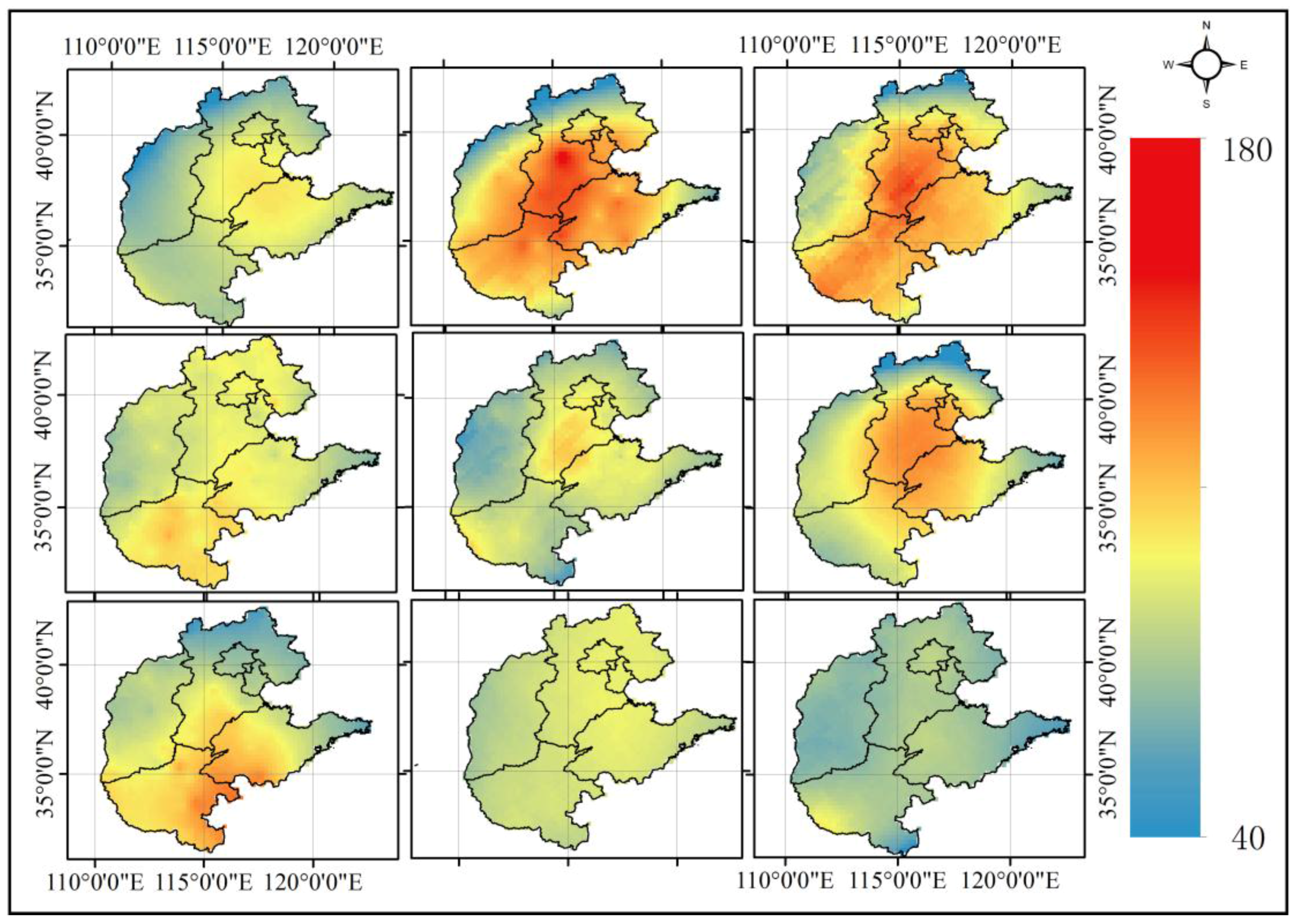
The distribution of AQI has obvious spatial characteristics. For the study area, the most polluted areas of air quality are concentrated in Beijing, the southern part of Tianjin, the central-southern part of Hebei, the central-northern part of Henan and the western part of Shandong.

(5)

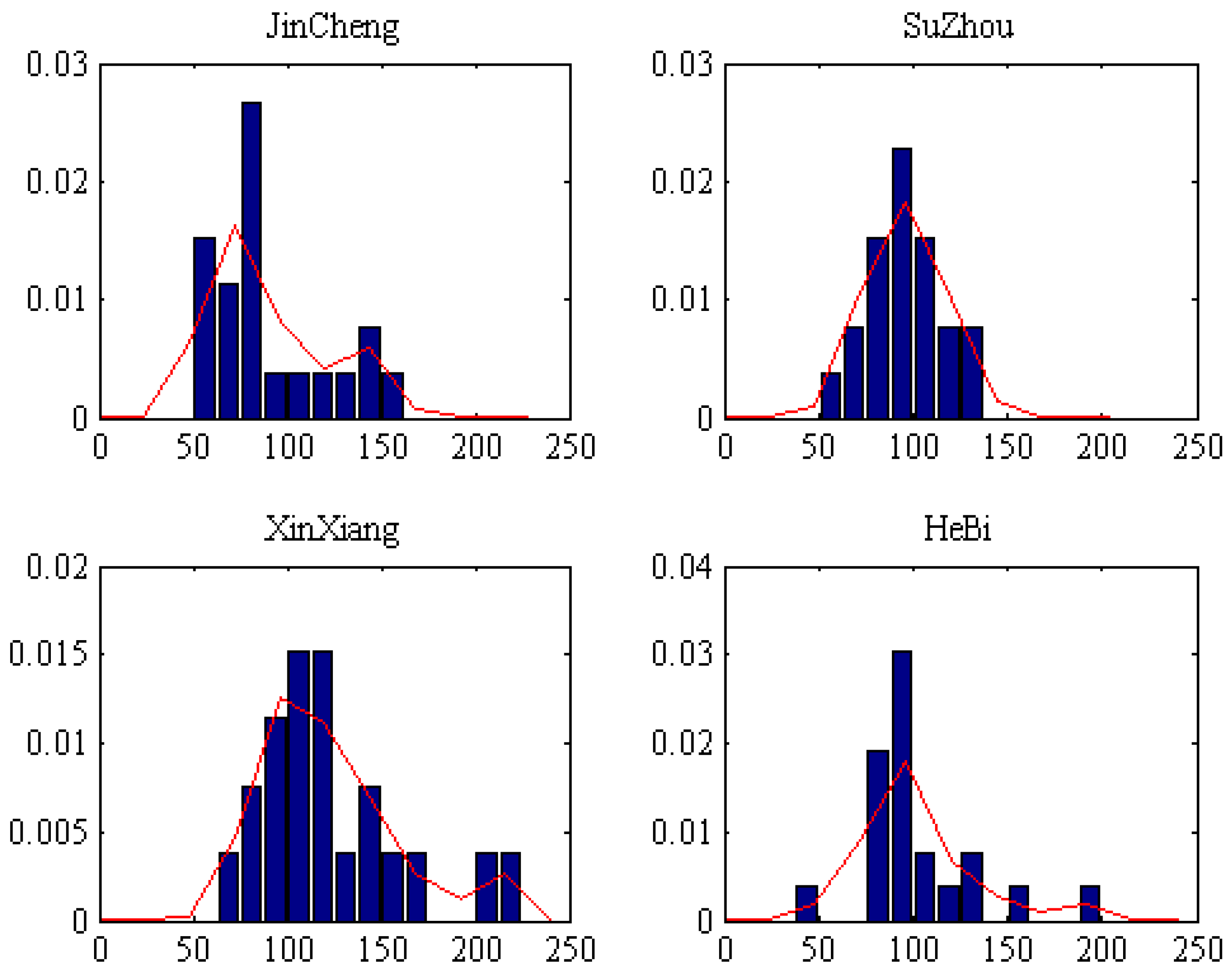
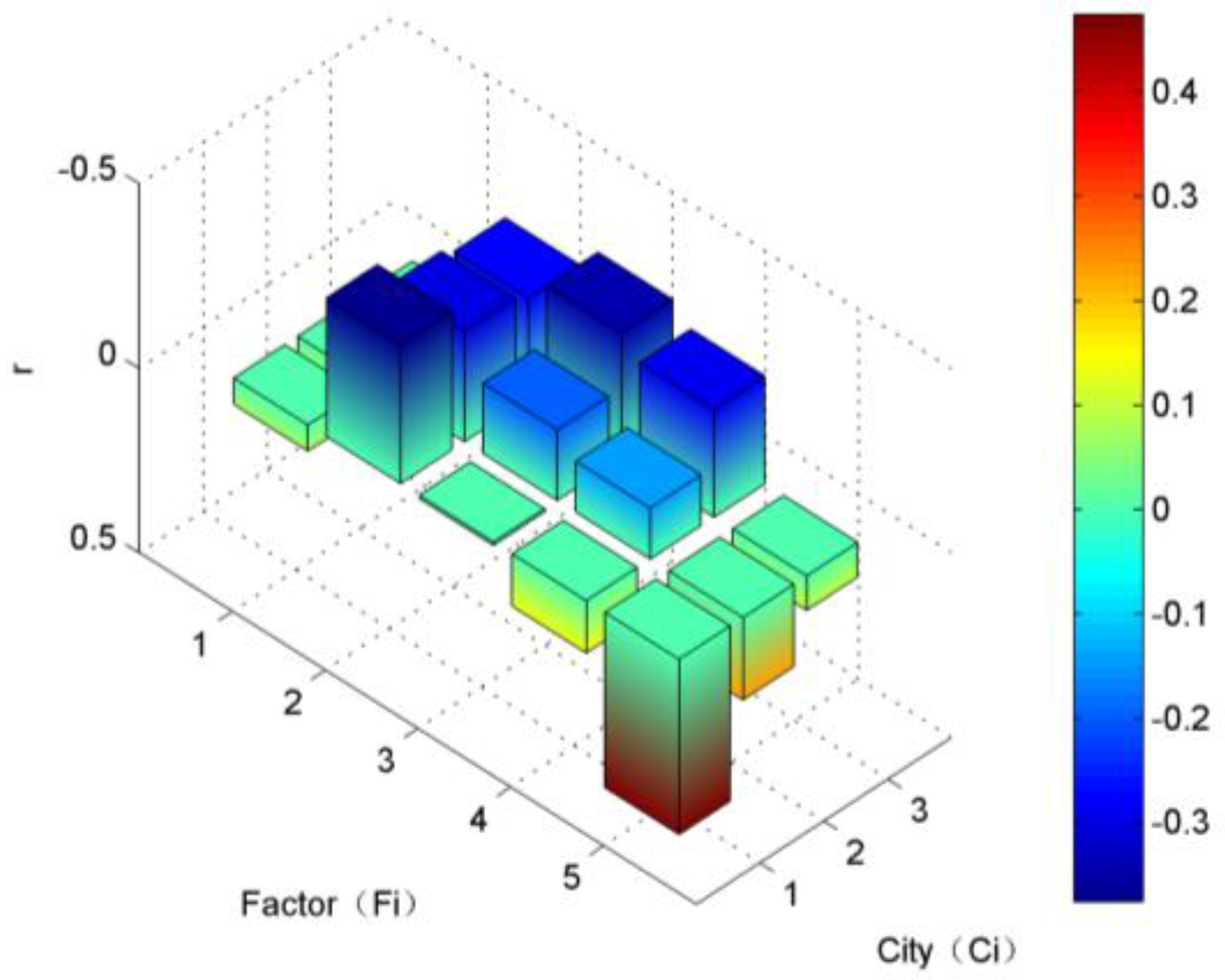
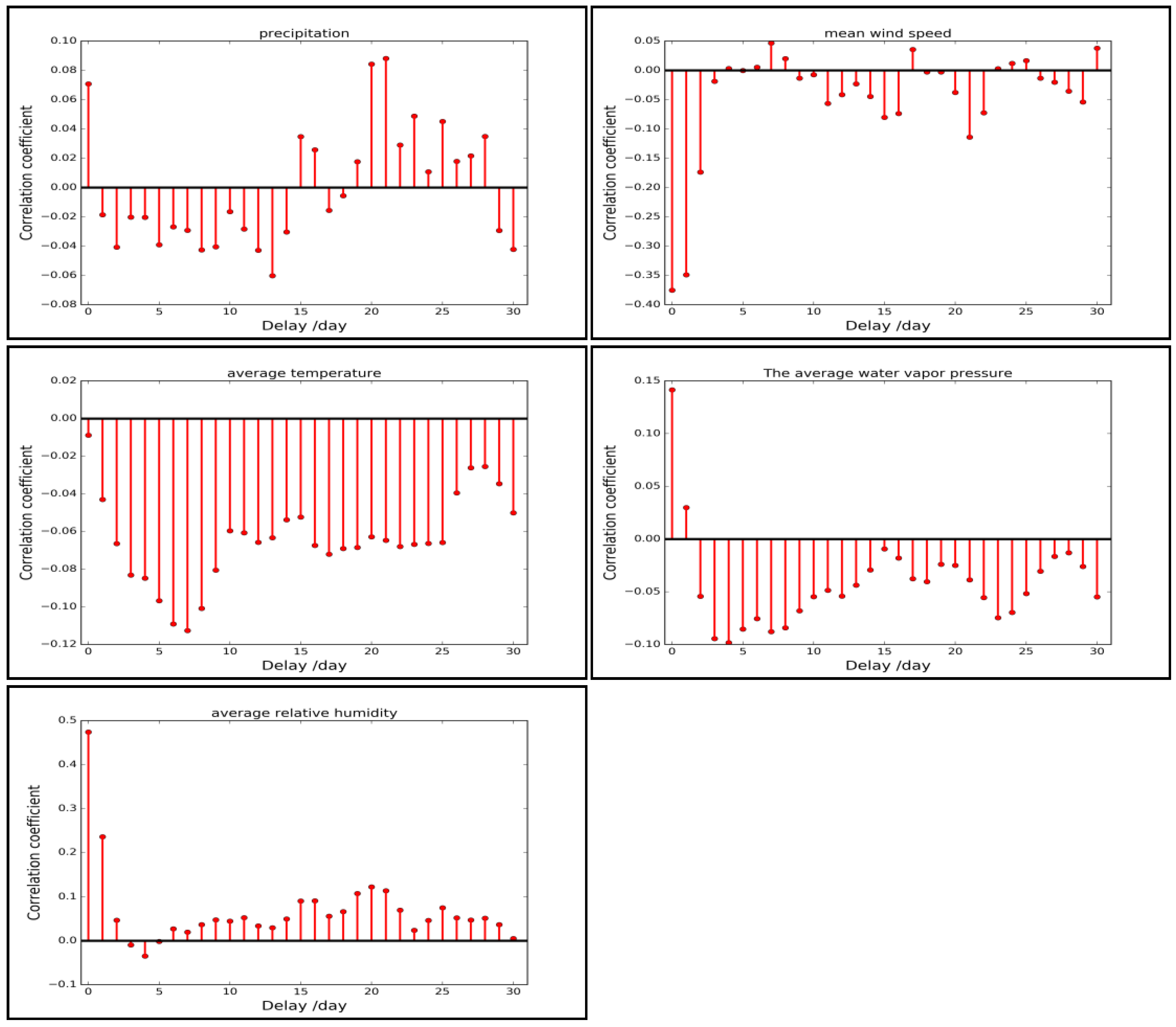
The average wind speed and average relative humidity have a real correlation. The calculated correlation coefficients using daily data provide support for association analysis on a finer scale. The effect of meteorological factors, such as wind, precipitation and humidity, on AQI is putative to have a temporal lag to different extents.

(6)

The AQI of a city with poor air quality will fluctuate greater than others when weather changes and has higher correlation with meteorological factors.

In subsequent studies, we should map the spatiotemporal distribution of AQI simultaneously, identify the patterns and explore the mechanism dominating the forming of the patterns. New interpolation techniques that are capable of incorporating uncertain data and dynamic mechanisms will be also devised to gain higher accuracy. Advanced methods appropriate for scale-variant detection of spatiotemporal patterns are imperative for addressing the inherent multi-scale problems in spatial data analysis.

References

1. Sæther, B.E.; Grøtan, V.; Tryjanowski, P. Climate and spatio-temporal variation in the population dynamics of a long distance migrant, the white stork. J. Anim. Ecol. 2006, 75, 80–90. [Google Scholar] [CrossRef] [PubMed]
2. Kyriakidis, P.C.; Journel, A.G. Stochastic modeling of atmospheric pollution: A spatial time-series framework. Part I: Methodology. Atmos. Environ. 2001, 35, 2331–2337. [Google Scholar] [CrossRef]
3. Varotsos, C.; Cartalis, C. Re-evaluation of surface ozone over Athens, Greece, for the period 1901–1940. Atmos. Res. 1991, 26, 303–310. [Google Scholar] [CrossRef]
4. Jacovides, C.P.; Varotsos, C.; Kaltsounides, N.A.; Petrakis, M.; Lalas, D.P. Atmospheric turbidity parameters in the highly polluted site of Athens basin. Renew. Energy 1994, 4, 465–470. [Google Scholar] [CrossRef]
5. Jacovides, C.P.; Karalis, J.D. Broad-band turbidity parameters and spectral band resolution of solar radiation for the period 1954–1991, in Athens, Greece. Int. J. Clim. 1996, 16, 229–242. [Google Scholar] [CrossRef]
6. Brook, R.D.; Franklin, B.; Cascio, W.; Hong, Y.; Howard, G.; Lipsett, M.; Luepker, R.; Mittleman, M.; Samet, J.; Smith, S.C.; et al. Air pollution and cardiovascular disease. Curr. Probl. Cardiol. 2012, 40, 207–238. [Google Scholar]
7. Wong, T.W.; Lau, T.S.; Yu, T.S.; Neller, A.; Wong, S.L.; Tam, W.; Pang, S.W. Air pollution and hospital admissions for respiratory and cardiovascular diseases in Hong Kong. Occup. Environ. Med. 1999, 56, 679–683. [Google Scholar] [CrossRef] [PubMed]
8. Barnett, A.G.; Williams, G.M.; Schwartz, J.; Best, T.L.; Neller, A.H.; Petroeschevsky, A.L.; Simpson, R.W. The Effects of Air Pollution on Hospitalizations for Cardiovascular Diseasein Elderly People in Australian and New Zealand Cities. Environ. Health Perspect. 2006, 114, 1018–1023. [Google Scholar] [CrossRef] [PubMed]
9. Koken, P.J.; Piver, W.T.; Ye, F.; Elixhauser, A.; Olsen, L.M.; Portier, C.J. Temperature, air pollution, and hospitalization for cardiovascular diseases among elderly people in Denver. Environ. Health Perspect. 2003, 111, 1312–1317. [Google Scholar] [CrossRef] [PubMed]
10. Feretis, E.; Theodorakopoulos, P.; Varotsos, C.; Efstathiou, M.; Tzanis, C.; Xirou, T.; Alexandridou, N.; Aggelou, M. On the plausible association between environmental conditions and human eye damage. Environ. Sci. Pollut. Res. 2002, 9, 163–165. [Google Scholar] [CrossRef]
11. Katsambas, A.; Andoniou, C.; Stratigos, J.; Arvanitis, I.; Zolota, F.; Varotsos, C.; Cartalis, C.; Asimakopoulos, D.N. A simple algorithm for simulating the solar ultraviolet radiation at the Earth’s surface: An application in determining the minimum erythema dose. Earth Moon Planets 1991, 53, 191–204. [Google Scholar] [CrossRef]
12. An, J.-L.; Wang, Y.-S.; Li, X.; Sun, Y.; Shen, S.H. Relationship between surface UV radiation and air pollution in Beijing. Environ. Sci. 2008, 29, 1053–1058. [Google Scholar]
13. Shi, Y. Ambient Air Quality Standard. J. China Environ. Manag. Cadre Coll. 2012, 1, 71. [Google Scholar]
14. Li, A.; Bo, Y. The interpolation of precipitation based on Bayesian Maximum Entropy. J. Desert Res. 2012, 32, 1408–1416. [Google Scholar]
15. Bao, Z.; Liu, T.; Luo, J. Analysis of the Space and Time Distribution of China’s Environmental Quality Index. Geomat. World 2014, 21, 17–21. [Google Scholar]
16. Zhang, B.; Li, W.; Yang, Y. The Bayesian Maximum Entropy geostatistical approach and its application in soil and environmental sciences. Acta Pedol. Sin. 2011, 48, 831–839. [Google Scholar]
17. Zhang, Y.; Yan, H. Analysis of influencing factor of air quality in Urumqi. Math. Pract. Theory 2015, 45, 149–154. [Google Scholar]
18. Ashraf, M.; Loftis, J.C.; Hubbard, K.G. Application of geostatistics to evaluate partial weather station networks. Agric. Forest Meteorol. 1997, 84, 255–271. [Google Scholar] [CrossRef]
19. Peng, S. Development of Spatio-Temporal Interpolation Methods for Meteorological Elements. Master Dissertation, Central South University, Changsha, China, 1 June 2010. [Google Scholar]
20. Bartier, P.M.; Keller, C.P. Multivariate interpolation to incorporate thematic surface data using inverse distance weighting (IDW). Comput. Geosci. 1996, 22, 795–799. [Google Scholar] [CrossRef]
21. Cressie, N. Spatial prediction and ordinary kriging. Math. Geosci. 1988, 20, 405–421. [Google Scholar] [CrossRef]
22. Pereira, J.J.; Schultz, E.T.; Auster, P.J. Geospatial analysis of habitat use in yellowtail flounder Limanda ferruginea on Georges Bank. Mar. Ecol. Prog. 2012, 468, 279–290. [Google Scholar] [CrossRef]
23. Zhang, F.S.; Zhong, S.B.; Yang, Z.T.; Sun, C.; Wang, C.L.; Huang, Q.Y. Spatial Estimation of Losses Attributable to Meteorological Disasters in a Specific Area (105.0° E–115.0° E, 25° N–35° N) Using Bayesian Maximum Entropy and Partial Least Squares Regression. Adv. Meteorol. 2016, 2016, 1–16. [Google Scholar] [CrossRef]
24. Christakos, G. A Bayesian/maximum-entropy view to the spatial estimation problem. Math. Geol. 1990, 22, 763–777. [Google Scholar] [CrossRef]
25. Christakos, G.; Serre, M.L. BME analysis of spatiotemporal particulate matter distributions in North Carolina. Atmos. Environ. 2000, 34, 3393–3406. [Google Scholar] [CrossRef]
26. Christakos, G.; Serre, M.L.; Kovitz, J.L. BME representation of particulate matter distributions in the state of California on the basis of uncertain measurements. J. Geophys. Res. Atmos. 2001, 106, 9717–9731. [Google Scholar] [CrossRef]
27. Xia, X.L.; Qi, Q.W.; Liang, H.; Zhang, A.; Jiang, L.; Ye, Y.; Liu, C.; Huang, Y. Pattern of Spatial Distribution and Temporal Variation of Atmospheric Pollutants during 2013 in Shenzhen, China. ISPRS Int. J. Geo-Inf. 2017, 6, 2. [Google Scholar] [CrossRef]
28. Matheron, G. The Intrinsic Random Functions and Their Applications. Adv. Appl. Probab. 1973, 5, 439–468. [Google Scholar] [CrossRef]
29. Bilonick, R.A. The space-time distribution of sulfate deposition in the northeastern United States. Atmos. Environ. 1985, 19, 1829–1845. [Google Scholar] [CrossRef]
30. Bilonick, R.A. Monthly hydrogen ion deposition maps for the northeastern US from July 1982 to September 1984. Atmos. Environ. 1988, 22, 1909–1924. [Google Scholar] [CrossRef]
31. Sampson, P.D.; Guttorp, P. Nonparametric Estimation of Nonstationary Spatial Covariance Structure. J. Am. Stat. Assoc. 1992, 87, 108–119. [Google Scholar] [CrossRef]
32. Dale, L.; Zimmerman, M.; Bridget, Z. A Comparison of Spatial Semivariogram Estimators and Corresponding Ordinary Kriging Predictors. Technometrics 1991, 33, 77–91. [Google Scholar]
33. Seymour, G. The Predictive Sample Reuse Method with Application. J. Am. Stat. Assoc. 1975, 70, 320–328. [Google Scholar]
34. Peng, B.; Zhong, S.; Su, X.; Li, X. Analysis on Rainfall Spatial Interpolation Precision in Lijiang River Basin. J. Meteorol. Res. Appl. 2011, 32, 30–33. [Google Scholar]
35. Ziegel, E.R.; Chatfield, C. The Analysis of Time Series. In The Analysis of Time Series; Chapman and Hall: Boca Raton, FL, USA, 2004; pp. 199–227. [Google Scholar]
36. Jabro, J.D.; Stevens, W.B.; Evans, R.G. Spatial Variability and Correlation of Selected Soil Properties in the Ap Horizon of a CRP Grassland. Appl. Eng. Agric. 2010, 26, 419–428. [Google Scholar] [CrossRef]
Figure 1. The study area, its location in China and the monitoring stations of the air quality index (AQI) to be used.
Ijgi 06 00052 g001
Figure 2. Flowchart of the analysis of AQI.
Ijgi 06 00052 g002
Figure 3. AQI trend curves from August 2014–August 2016. (a) Beijing, Tianjin, Hebei (b) Henan; (c) Shanxi; and (d) Shandong. Date format: yyyy/mm.
Ijgi 06 00052 g003aIjgi 06 00052 g003b
Figure 4. AQI radar map. (a) AQI from August 2014–July 2015 and (b) from August 2015–July 2016.
Ijgi 06 00052 g004
Figure 5. AQI distribution map using inverse distance weighted (IDW) (the figure panel is read from left to right, from top to bottom: August 2014, November 2014, February 2015, May 2015, August 2015, November 2015, February 2016, May 2016, August 2016).
Ijgi 06 00052 g005
Figure 6. The distribution investigation of AQI data with several ESDA (exploratory spatial data analysis) techniques, such as histogram, quantile-quantile (Q-Q) diagram and 3D scatterplot. (a) Distribution histogram; (b) normal Q-Q plot; and (c) trend analysis.
Ijgi 06 00052 g006
Figure 7. The empirical semivariogram models for nine selected months (the figure panel is read from left to right, from top to bottom: August 2014, November 2014, February 2015, May 2015, August 2015, November 2015, February 2016, May 2016, August 2016).
Ijgi 06 00052 g007aIjgi 06 00052 g007b
Figure 8. AQI distribution map using ordinary kriging (the figure panel is read from left to right, from top to bottom: August 2014, November 2014, February 2015, May 2015, August 2015, November 2015, February 2016, May 2016, August 2016).
Ijgi 06 00052 g008
Figure 9. The probability density function of partial stations.
Ijgi 06 00052 g009
Figure 10. AQI distribution map using Bayesian maximum entropy (the figure panel is read from left to right, from top to bottom: August 2014, November 2014, February 2015, May 2015, August 2015, November 2015, February 2016, May 2016, August 2016).
Ijgi 06 00052 g010
Figure 11. The accuracy of each interpolation method. (a) August 2014; (b) November 2014; (c) February 2015; (d) May 2015; (e) August 2015; (f) November 2015; (g) February 2016; (h) May 2016; and (i) August 2016.
Ijgi 06 00052 g011
Figure 12. Temporal correlation analysis between meteorological factors and AQI in Beijing.
Ijgi 06 00052 g012
Figure 13. Temporal correlation analysis in Beijing, Tianjin and Zhengzhou. Ci = [Beijing, Tianjin, Zhengzhou], Fi = [precipitation anomaly percentage, precipitation, mean wind speed, average temperature, average water vapor pressure, average relative humidity].
Ijgi 06 00052 g013
Figure 14. Temporal correlation analysis between daily meteorological factors and AQI in Beijing.
Ijgi 06 00052 g014
Figure 15. Temporal correlation analysis in Beijing, Tianjin and Zhengzhou. Ci = [Beijing, Tianjin, Zhengzhou], Fi = [precipitation, mean wind speed, average temperature, average water vapor pressure, average relative humidity].
Ijgi 06 00052 g015
Figure 16. Temporal cross-correlation analysis between daily meteorological factors and AQI in Beijing considering temporal lag.
Ijgi 06 00052 g016