
Building an Urban Spatial Structure from Urban Land Use Data: An Example Using Automated Recognition of the City Centre


Abstract
:1. Introduction
2. Related Work
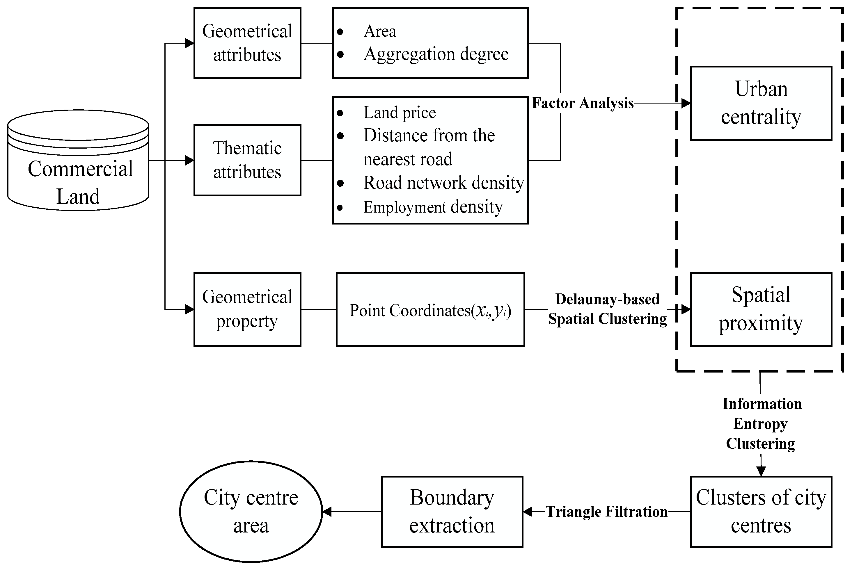
3. Methodology
3.1. Detecting Clusters Using a Graph-Based Spatial Clustering Algorithm
3.1.1. Construction of Spatial Proximity Relationships
3.1.2. Clustering Commercial Lands with Attribute Similarity
3.1.3. Algorithm Description
Determination of the Attribute Clustering Threshold
Detection of Clusters Using Our Spatial Clustering Algorithm
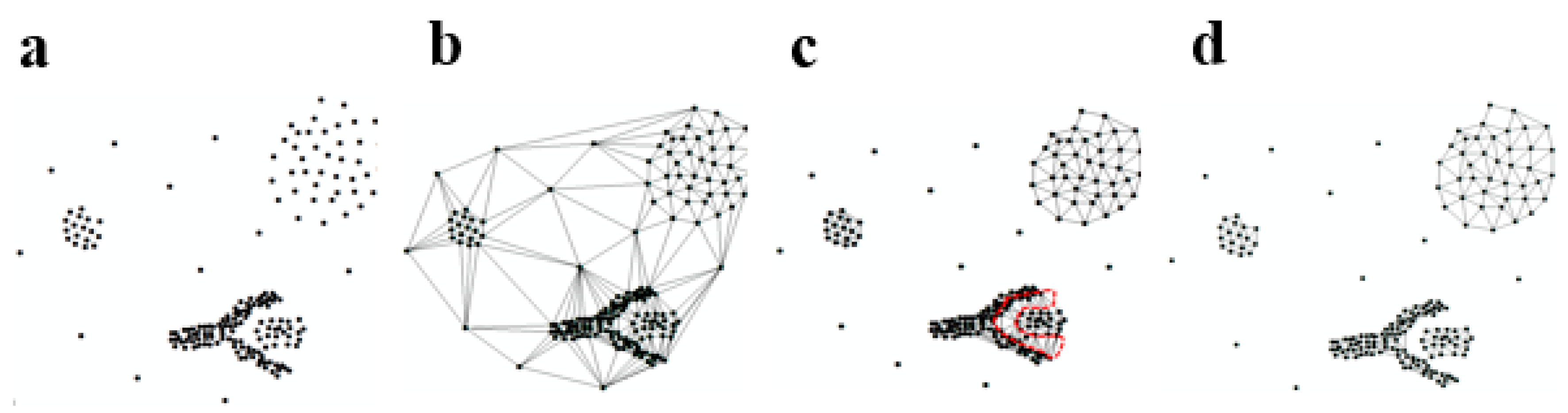
- ①
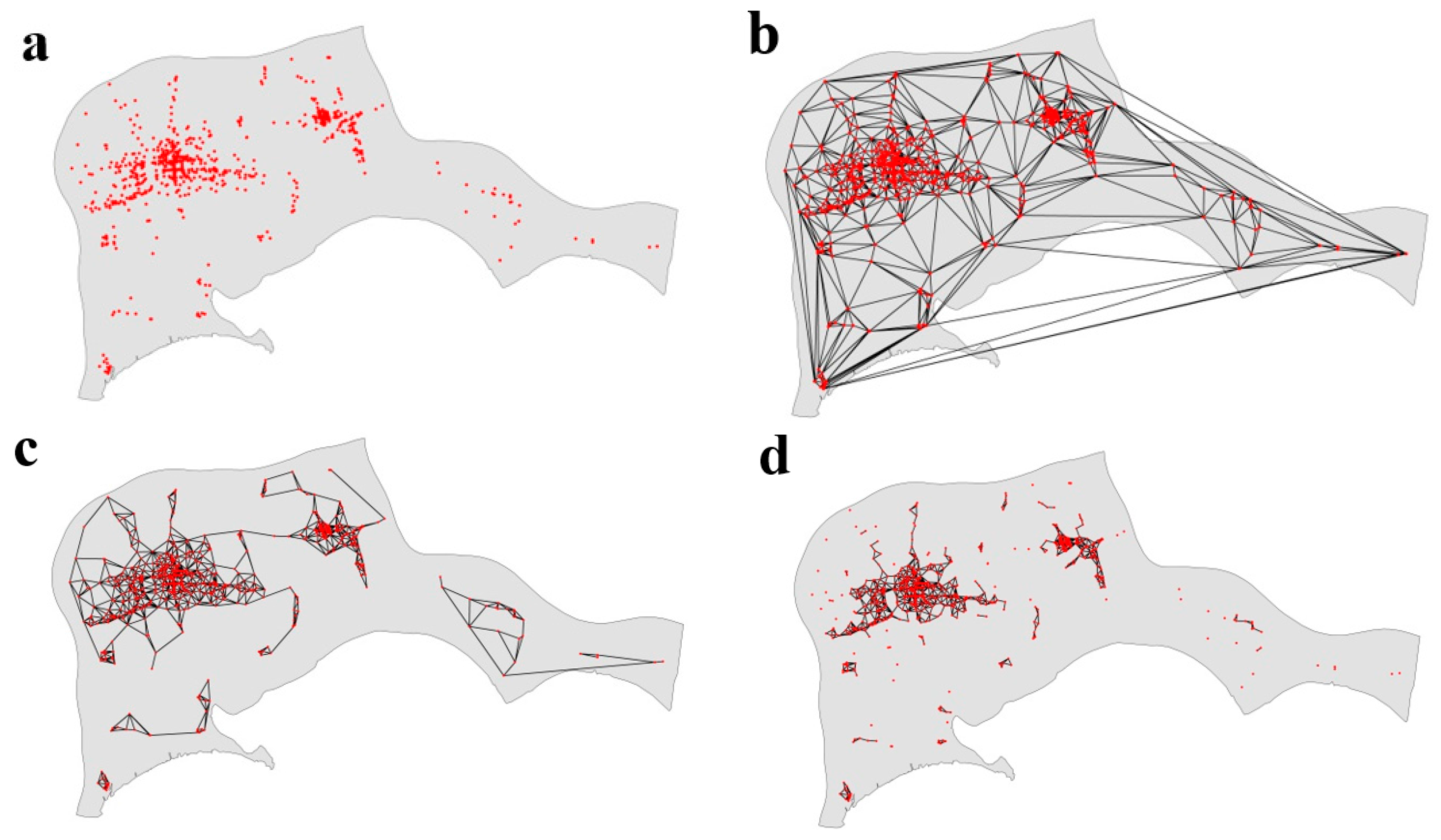
- Convert commercial land blocks into discrete points, and then construct Delaunay triangulation for these points.
- ②
- Remove the edges from the Delaunay triangulation using global edge-length constraints.
- ③
- Remove the edges from the Delaunay triangulation using local edge-length constraints.
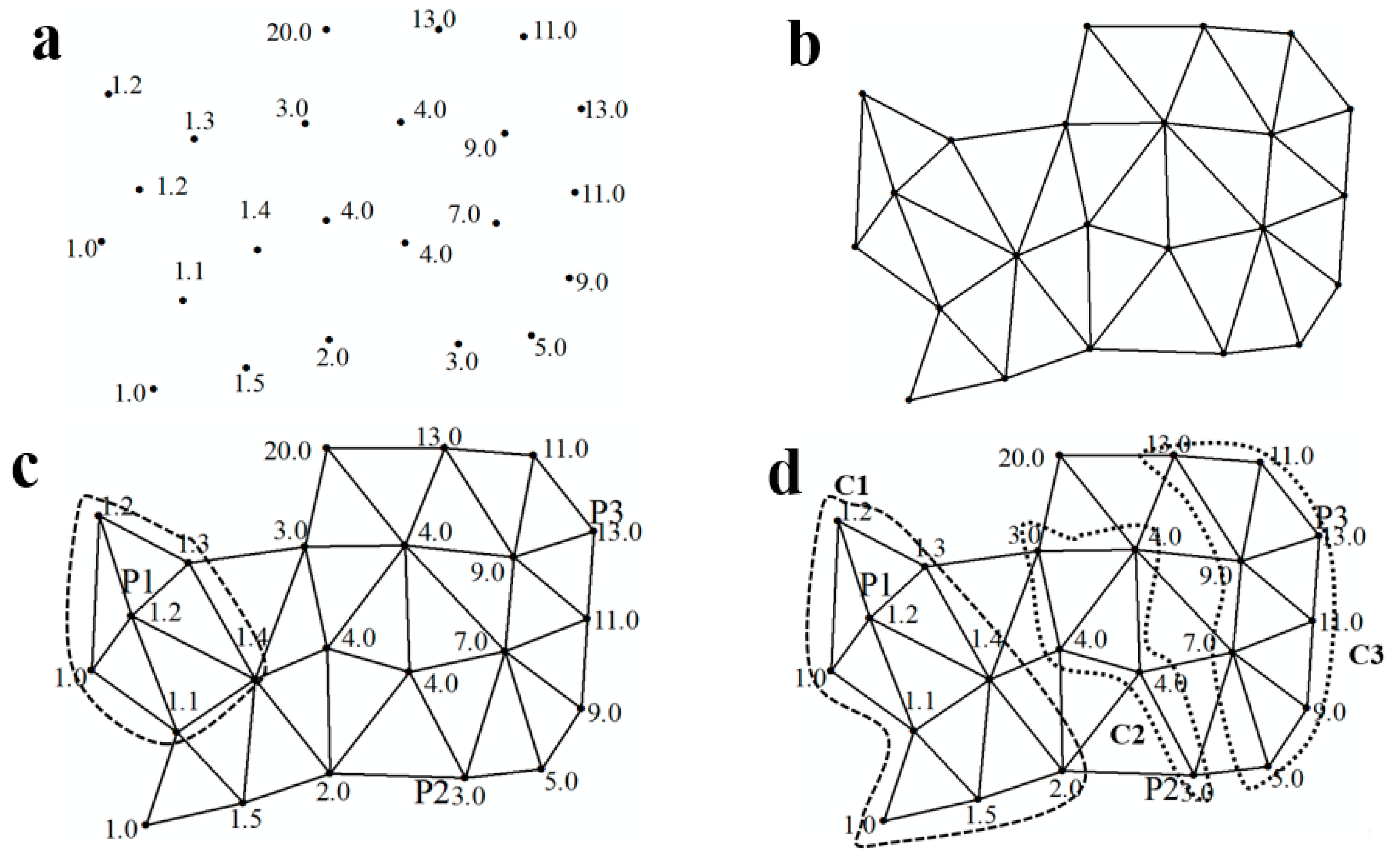
- ①
- Select the maximum value of the neighbourhood entropy as .
- ②
- Use the breadth-first search to visit directly and indirectly adjacent neighbours of in descending order of their neighborhood entropy. The cluster is formed if they satisfy Formula (15) and no new object is added to the cluster, thus identifying them as clustered.
- ③
- Traverse all points that are not clustered by iterating operations (1)–(2). When clustering is finished, any point that does not belong to a cluster will be identified as noise.
3.1.4. Algorithm Analysis
Implementation Procedure of the Algorithm
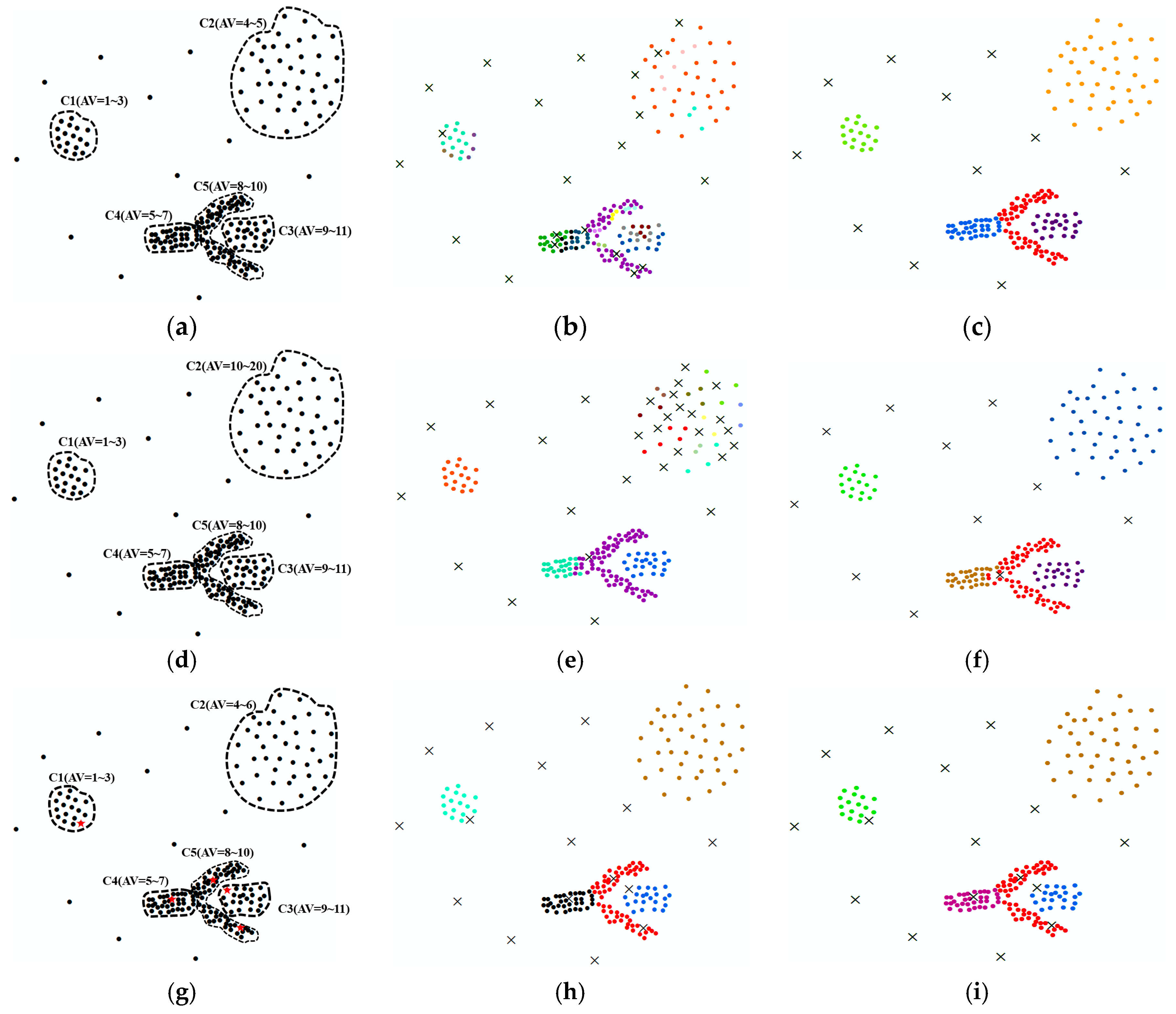
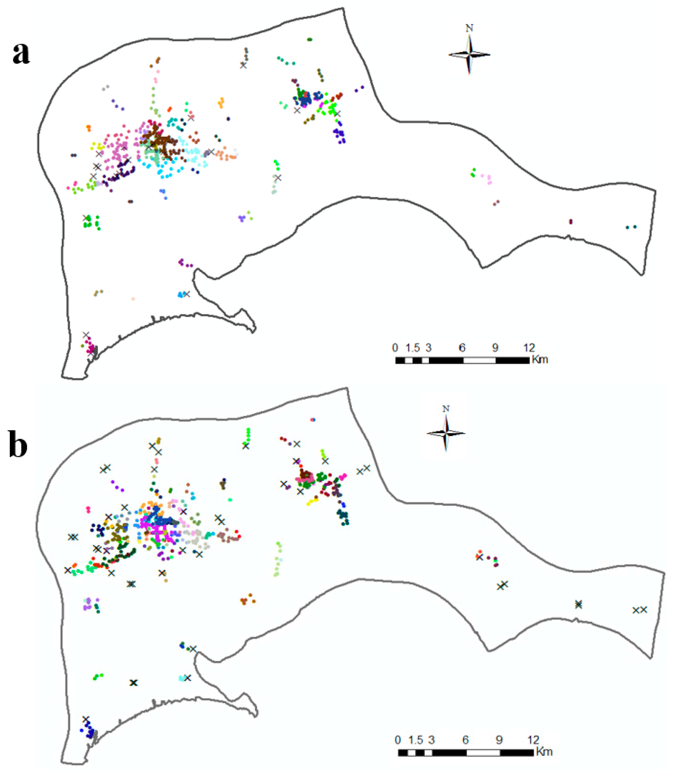
Algorithm Validation
 ), with the attribute values of outliers randomly set from 40 to 60. As seen in Figure 4h, i, our method and the DBSC algorithm could separate five clusters and outliers very well.
3.2. Characterising the City Center
3.2.1. Extraction of Indicators
- (1)
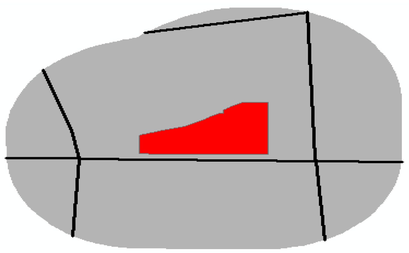
- Aggregation degree of commercial land. The distribution of commercial land in city centre areas tends to be clustered, and the area of each commercial plot cannot measure the unequal distribution of commercial land. Therefore, we considered the area and space occupied by commercial land, to measure the aggregation degree of commercial land. We used an approach provided by Ai and Van Oosterom [51] to compute the space occupied by commercial land. A geometric construction similar to a Voronoi diagram was created based on the skeleton of the Delaunay triangulation built using a polygon (commercial land) boundary, as shown in Figure 5a. The aggregation degree of commercial land is expressed aswhere denotes a commercial plot, denotes the aggregation degree of , denotes the area of , and denotes the area of space occupied by . The range of is 0 to 1. If tends to 1, then the distribution of commercial land is clustered. The higher clustering of commercial plots was in the city centre areas, as shown in Figure 5b (Region 1). In contrast, when tended to 0, the distribution of commercial land was decentralized, as shown in Figure 5b (Region 2).
- (2)
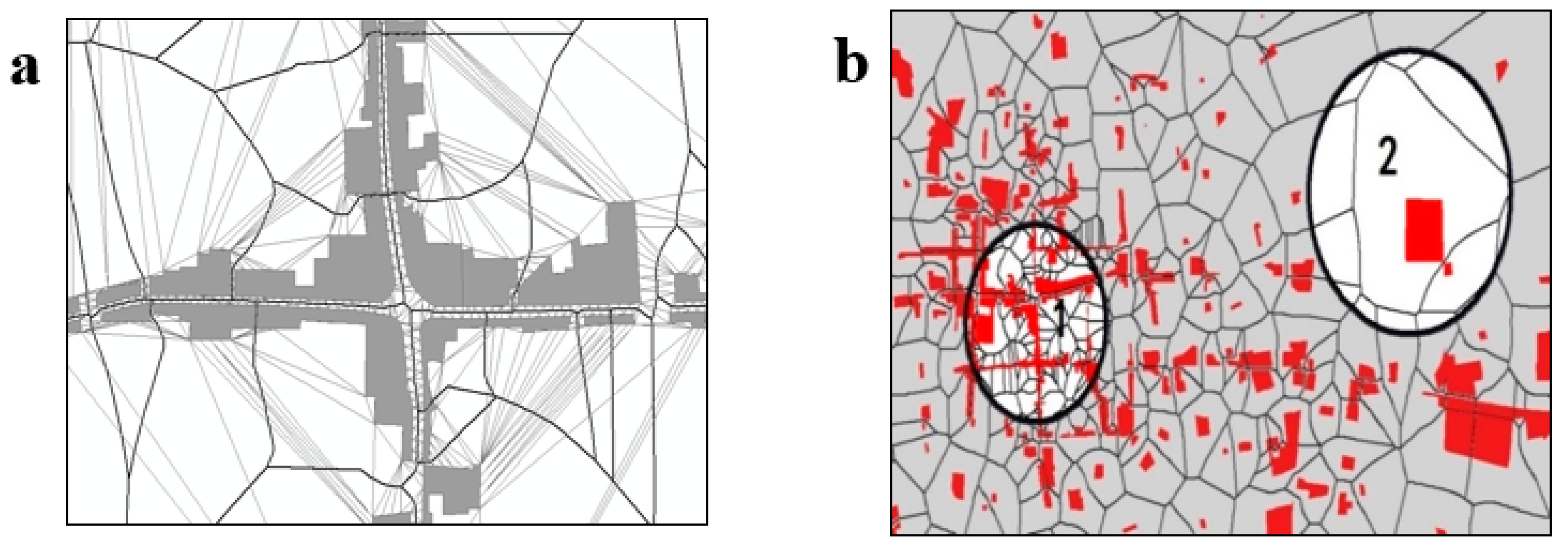
- Road network density and distance from the nearest road. Many urban districts with high commercial functions have been formed around the road network. Those regions feature high accessibility, namely, the comercial lands located in the city centre areas show higher accessibility. Road network density and distance from the nearest trunk road are important indicators for measuring accessibility. To compute the road network density for commercial land, the buffer operation of GIS was used to determine for how long the roads are located in a circular area with a radius distance of 1 km within the commercial land, as shown in Figure 6. Therefore,where denotes a commercial plot, denotes the road network density of , denotes the buffer area of (the buffer radius is usually set to 1 km), and denotes the sum length of roads that are located inside the circular area of the commercial plot.
- (3)
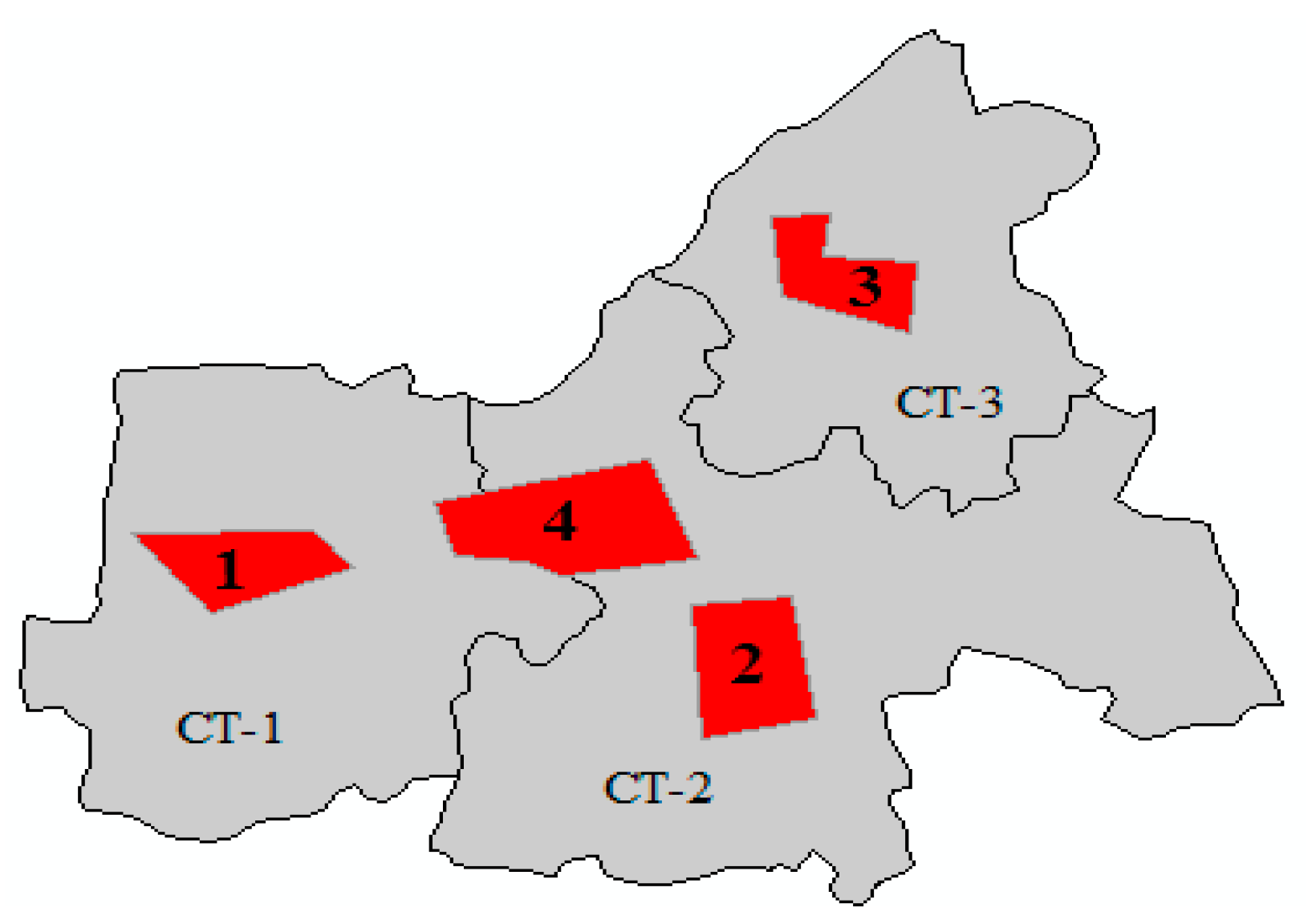
- Employment density. Broadly, the distribution of employment data was used to identify city centres. Conventionally, employment density obtained from the census tract failed to meet our statistical zone (i.e., commercial land). We computed the employment density of commercial land as the density of the census tract if the primary part of the commercial land fell into this census tract. As shown in Figure 7, the employment density of commercial land 1, 2 and 3 was, respectively, the density of CT-1, CT-2 and CT-3. The value of commercial land 4 should have been the same as commercial land 2 because the primary part of the commercial land fell into CT-2.
3.2.2. Index of Urban Centrality
3.3. Extracting the City Centre Area
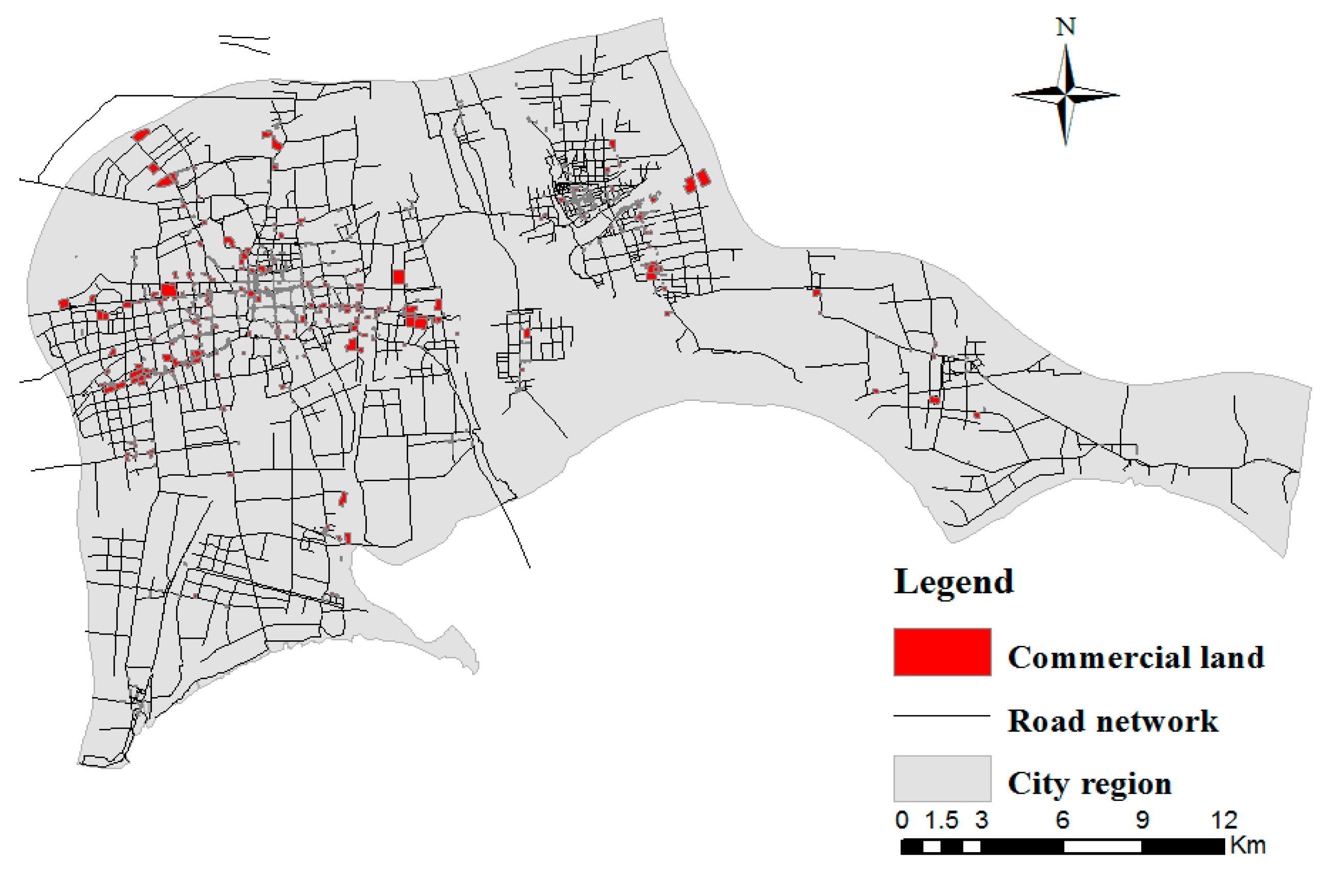
4. Application
4.1. Construction of Spatial Proximity Relationships
4.2. Clustering Commercial Lands with Attribute Similarity
4.2.1. Using the Factor Analysis Method for the Index of Urban Centrality
4.2.2. Clustering Commercial Land with Attributes
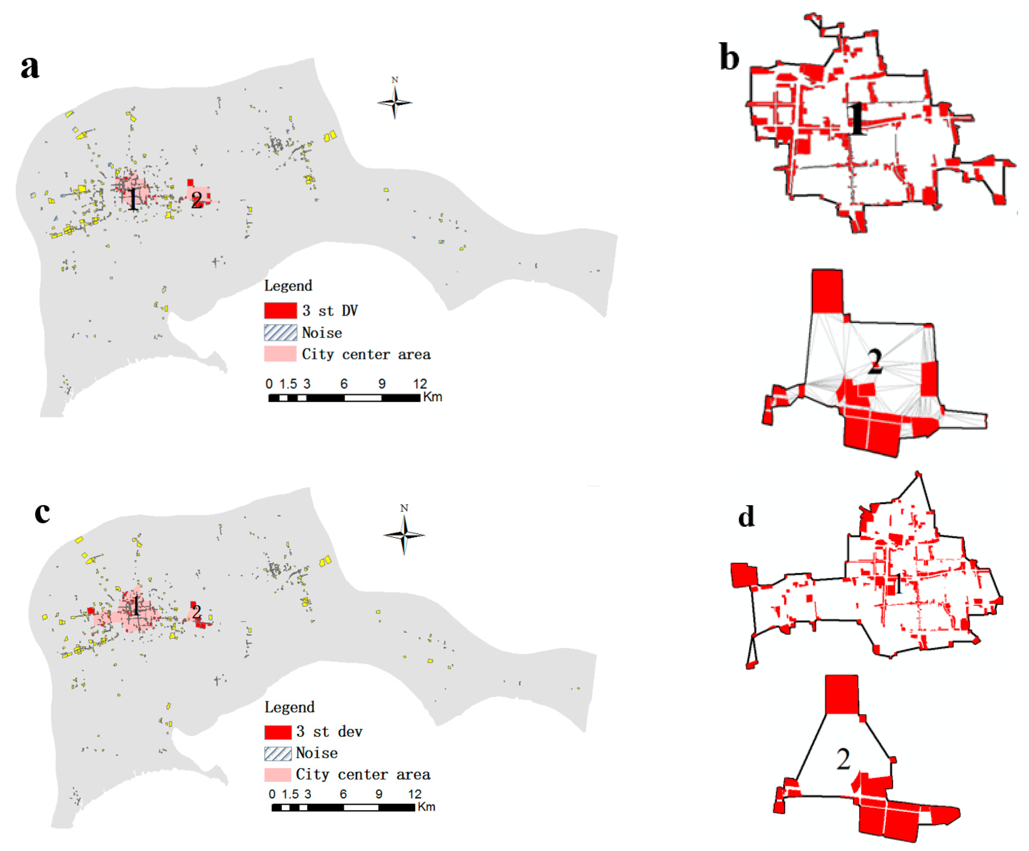
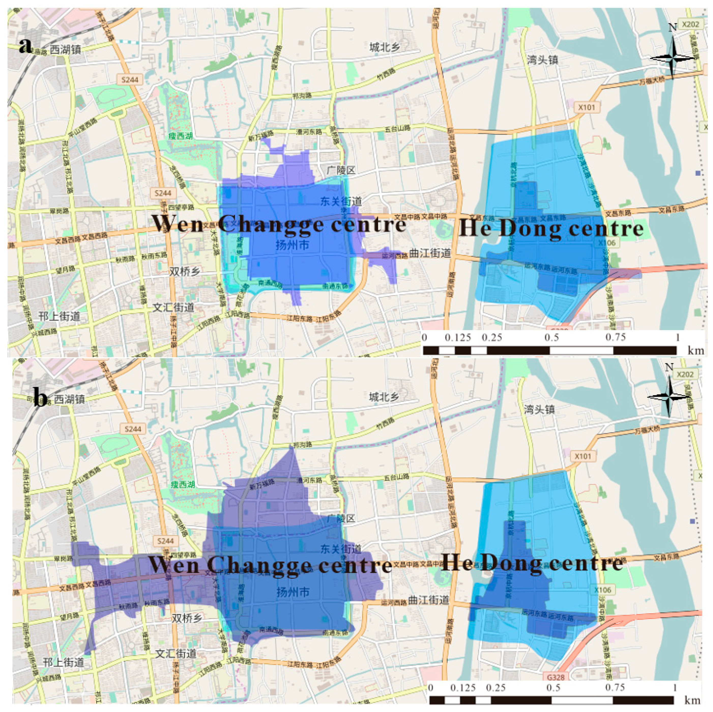
4.3. Results and Validation
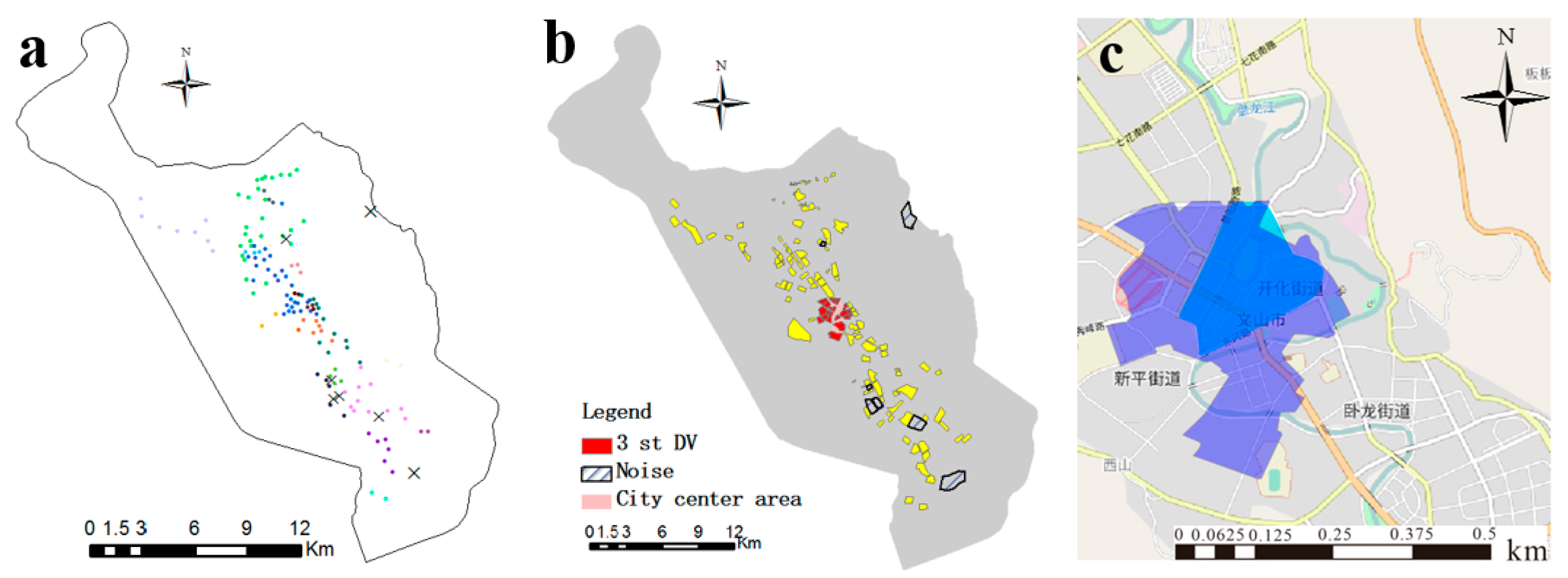
4.4. Case study of Wenshan
5. Conclusions and Outlooks
Acknowledgments
Author Contributions
Conflicts of Interest
References
- Bourne, L.S. Internal structure of the city: Readings on urban form, growth, and policy. Historian 1963, 26, 1–18. [Google Scholar]
- Yoshida, H.; Omae, M. An approach for analysis of urban morphology: Methods to derive morphological properties of city blocks by using an urban landscape model and their interpretations. Comput. Environ. Urban Syst. 2005, 29, 223–247. [Google Scholar] [CrossRef]
- Ariza-Villaverde, A.B.; Jiménez-Hornero, F.J.; Ravé, E.G.D. Multifractal analysis of axial maps applied to the study of urban morphology. Comput. Environ. Urban Syst. 2013, 38, 1–10. [Google Scholar] [CrossRef]
- Wang, L. Object-based spatial cluster analysis of urban landscape pattern using nighttime light satellite images: A case study of China. Int. J. Geogr. Inf. Sci. 2014, 28, 2328–2355. [Google Scholar]
- Zhang, L.Q.; Shu, J. A GIS-based gradient analysis of the urban landscape pattern of shanghai metropolitan region. Acta Polym. Sin. 2004, 28, 78–85. [Google Scholar]
- Faris, J.M.; Beever, L.B.; Brown, M. Geography Information System (GIS) and Urban Land Use Allocation Model (ULAM) techniques for existing and projected land use data. In Proceedings of the seventh National Conference on Transportation Planning for Small and Medium-Sized Communities, Little Rock, AR, USA, 28–30 September 2000. [Google Scholar]
- Haque, A.; Asami, Y. Optimizing urban land use allocation for planners and real estate developers. Comput. Environ. Urban Syst. 2014, 46, 57–69. [Google Scholar] [CrossRef]
- Feng, Y.; Liu, Y.; Tong, X.; Liu, M.; Deng, S. Modeling dynamic urban growth using cellular automata and particle swarm optimization rules. Landsc. Urban Plan. 2011, 102, 188–196. [Google Scholar] [CrossRef]
- Jafari, M.; Majedi, H.; Monavari, S.M.; Alesheikh, A.A.; Kheirkhah Zarkesh, M. Dynamic simulation of urban expansion based on cellular automata and logistic regression model: Case study of the Hyrcanian Region of Iran. Sustainability 2016, 8, 810. [Google Scholar] [CrossRef]
- Lüscher, P.; Weibel, R. Exploiting empirical knowledge for automatic delineation of city centres from large-scale topographic databases. Comput. Environ. Urban Syst. 2013, 37, 18–34. [Google Scholar] [CrossRef]
- Egenhofer, M.J.; Mark, D.M. Naive geography. In Spatial Informat-Ion Theory. A Theoretical Basis for GIS. Proceeding of the Sinternational Conference COSIT ’95; Frank, A.U., Kuhn, W., Eds.; Springer: Berlin, Germany, 1995; pp. 21–23. [Google Scholar]
- Yu, W.; Ai, T.; Shao, S. The analysis and delimitation of Central Business District using network kernel density estimation. J. Transp. Geogr. 2015, 45, 32–47. [Google Scholar] [CrossRef]
- Murphy, R.E.; Vance, J.E. Delimiting the CBD. Econ. Geol. 1954, 30, 189–222. [Google Scholar] [CrossRef]
- Eubank, S.; Guclu, H.; Kumar, V.S.; Marathe, M.V.; Srinivasan, A.; Toroczkai, Z.; Wang, N. Modelling disease outbreaks in realistic urban social networks. Nature 2004, 429, 180–184. [Google Scholar] [CrossRef] [PubMed]
- Wang, P.; González, M.C.; Hidalgo, C.A.; Barabási, A.-L. Understanding the Spreading Patterns of Mobile Phone Viruses. Science 2009, 324, 1071–1076. [Google Scholar] [CrossRef] [PubMed]
- Zhang, C. An analysis of urban spatial structure using comprehensive prominence of irregular areas. Int. J. Geogr. Inf. Sci. 2008, 22, 675–686. [Google Scholar] [CrossRef]
- Alonso, W. A theory of the urban land market. Pap. Pro. Reg. Sci. Assoc. 1960, 6, 149–157. [Google Scholar] [CrossRef]
- Martin, D.; Higgs, G. Population georeferencing in England and Wales: Basic spatial units reconsidered. Environ. Plann. A 1997, 29, 333–347. [Google Scholar] [CrossRef]
- Baumont, C.; Ertur, C.; Gallo, J. Spatial analysis of employment and population density: The case of the agglomeration of Dijon 1999. Geogr. Anal. 2004, 36, 146–176. [Google Scholar] [CrossRef]
- Yang, X.; Huang, Y.; Dong, P.; Jiang, D.; Liu, H. An updating system for the gridded population database of China based on remote sensing, GIS and spatial database technologies. Sensors 2009, 9, 1128–1140. [Google Scholar] [CrossRef] [PubMed]
- Ord, J.K,; Getis, A. Local Spatial Autocorrelation Statistics: Distributional Issues and an Application. Geogr. Anal. 1995, 27, 286–306. [Google Scholar] [CrossRef]
- Roth, C.; Kang, S.M.; Batty, M.; Barthélemy, M. Structure of Urban Movements: Polycentric Activity and Entangled Hierarchical Flows. PLoS ONE 2010, 6, e15923. [Google Scholar] [CrossRef] [PubMed]
- Zhou, X.; Liu, J.; Yeh, A.G.O.; Yue, Y.; Li, W. The uncertain geographic context problem in identifying activity centers using mobile phone positioning data and point of interest data. In Advances in Spatial Data Handling and Analysis; Springer: Berlin, Germany, 2015; pp. 107–119. [Google Scholar]
- Taubenböck, H.; Klotz, M.; Wurm, M.; Schmieder, J.; Wagner, B.; Wooster, M.; Esch, T.; Dech, S. Delineation of Central Business Districts in Mega city regions using remotely sensed data. Remote Sens. Environ. 2013, 136, 386–401. [Google Scholar] [CrossRef]
- Galster, G.; Hanson, R.; Ratcliffe, M.R.; Wolman, H.; Coleman, S.; Freihage, J. Wrestling sprawl to the ground: Defining and measuring an elusive concept. Hous Policy Debate 2001, 12, 681–717. [Google Scholar] [CrossRef]
- Lee, B. Urban Spatial Structure, Commuting, and Growth in US Metropolitan Areas. Ph.D. Thesis, University of Southern California, Los Angeles, CA, USA, 2006. [Google Scholar]
- Pereira, R.H.M.; Nadalin, V.; Monasterio, L.; Albuquerque, P.H. Urban centrality: A simple index. Geogr. Anal. 2013, 45, 77–89. [Google Scholar] [CrossRef]
- Berrill, K.; Florence, P.S.; Baldamus, W. Investment, Location, and Size of Plant. Econ. Stat. 1948, 58, 411–414. [Google Scholar]
- Midelfart-Knarvik, K.H.; Venables, A.J. Integration and industrial specialization in the European Union. Rev. Econ. 2002, 53, 469–482. [Google Scholar]
- Tsai, Y.-H. Quantifying urban form: Compactness versus sprawl. Urban Stud. 2005, 42, 141–161. [Google Scholar] [CrossRef]
- Thurstain-Goodwin, M.; Unwin, D. Defining and delineating the central areas of towns for statistical monitoring using continuous surface representations. Trans. GIS 2000, 4, 305–317. [Google Scholar] [CrossRef]
- Borruso, G. Network density and the delimitation of urban areas. Trans. GIS 2003, 7, 177–191. [Google Scholar] [CrossRef]
- Battaglia, F.; Borruso, G.; Porceddu, A. Real Estate values, urban centrality, economic activities. A GIS Analysis on the City of Swindon (UK). In Proceedings of the 10th Computational Science and Its Applications–ICCSA, Fukuoka, Japan, 23–26 March 2010. [Google Scholar]
- Hollenstein, L.; Purves, R. Exploring place through user-generated content: Using Flickr to describe city cores. J. Spat. Inf. Sci. 2010, 1, 21–48. [Google Scholar]
- Borruso, G.; Porceddu, A. A Tale of Two Cities: Density Analysis of CBD on Two Midsize Urban Areas in Northeastern Italy. In Geocomputation and Urban Planning; Springer: Berlin, Germany, 2009; pp. 37–56. [Google Scholar]
- Battino, S.; Borruso, G.; Donato, C. Analyzing the central business district: The case of sassari in the sardinia island. In Proceedings of the 12th Computational Science and Its Applications–ICCSA, Salvador de Bahia, Brazil, 18–21 June 2012. [Google Scholar]
- Hu, Y.; Gao, S.; Janowicz, K.; Yu, B.; Li, W.; Prasad, S. Extracting and understanding urban areas of interest using geotagged photos. Comput. Environ. Urban Syst. 2015, 54, 240–254. [Google Scholar] [CrossRef]
- Sun, Y.; Fan, H.; Li, M.; Zipf, A. Identifying the city center using human travel flows generated from location-based social networking data. Environ. Plann. B 2016, 43, 480–498. [Google Scholar] [CrossRef]
- Montello, D.R.; Goodchild, M.F.; Gottsegen, J.; Fohl, P. Where‘s downtown: Behavioral methods for determining referents of vague spatial queries. Spat. Cognit. Comput. 2003, 3, 185–204. [Google Scholar] [CrossRef]
- Henderson, M.; Yeh, E.T.; Gong, P.; Elvidge, C.; Baugh, K. Validation of urban boundaries derived from global night-time satellite imagery. Int. J. Remote. Sens. 2003, 24, 595–609. [Google Scholar] [CrossRef]
- Estivill-Castro, V.; Lee, I. Argument free clustering for large spatial point-data sets via boundary extraction from Delaunay Diagram. Comput. Environ. Urban Syst. 2002, 26, 315–334. [Google Scholar] [CrossRef]
- Liu, Q.; Deng, M.; Shi, Y.; Wang, J. A density-based spatial clustering algorithm considering both spatial proximity and attribute similarity. Comput. Geosci. 2012, 46, 296–309. [Google Scholar] [CrossRef]
- Liu, D.; Sourina, O. Free-parameters clustering of spatial data with non-uniform density. In Proceedings of the 2004 IEEE Conference on Cybernetics and Intelligent Systems, Singapore, 1–3 December 2004. [Google Scholar]
- Ester, M.; Kriegel, H.P.; Sander, J.; Xu, X. A density-based algorithm fordiscovering clusters in large spatial databases with noise. In Proceedings of the 2nd International Conference on Knowledge Discovery and Data Mining, Portland, OR, USA; 1996; pp. 226–231. [Google Scholar]
- Shannon, C.E. A mathematical theory of communication. ACM SIGMOBILE Mob. Comput. Commun. Rev. 2001, 5, 3–55. [Google Scholar] [CrossRef]
- Cormen, T.H.; Leiserson, C.E.; Rivest, R.L. Introduction to Algorithms; MIT Press, Inc.: Cambridge, MA, USA, 1990. [Google Scholar]
- Pakhira, M.K.; Bandyopadhyay, S.; Maulik, U. Validity index for crisp and fuzzy clusters. Pattern Recogn. 2004, 37, 487–501. [Google Scholar] [CrossRef]
- Gordon, P.; Richardson, H.W.; Wong, H.L. The distribution of population and employment in a polycentric city: The case of Los Angeles. Environ. Plann. A 1986, 18, 161–173. [Google Scholar] [CrossRef]
- Yan, X.; Zhou, C.; Leng, Y.; Chen, H. Functional features and spatial structure of CBDs in Guangzhou. Acta Geogr. Sin. 2000, 55, 475–486. [Google Scholar]
- Wu, M.W. Urban Central District Planning; Southeast University Press: Nanjing, China, 2009. (In Chinese) [Google Scholar]
- Ai, T.; Van Oosterom, P. GAP-tree extensions based on skeletons. In Advances in Spatial Data Handling; Springer: Berlin, Germany, 2002; pp. 501–513. [Google Scholar]
- Kline, P. An Easy Guide to Factor Analysis; Routledge: London, UK, 2014. [Google Scholar]
- Chainey, S.; Reid, S.; Stuart, N. When is a hotspot a hotspot? A procedure forcreating statistically robust hotspot maps of crime. In Socio-Economic Applications of Geographic InformationScience; Kidner, D., Higgs, G., White, S., Eds.; Taylor and Francis: London, UK, 2002; pp. 21–36. [Google Scholar]
- Peethambaran, J.; Muthuganapathy, R. A non-parametric approach to shape reconstruction from planar point sets through Delaunay filtering. Comput. Aided Des. 2015, 62, 164–175. [Google Scholar] [CrossRef]


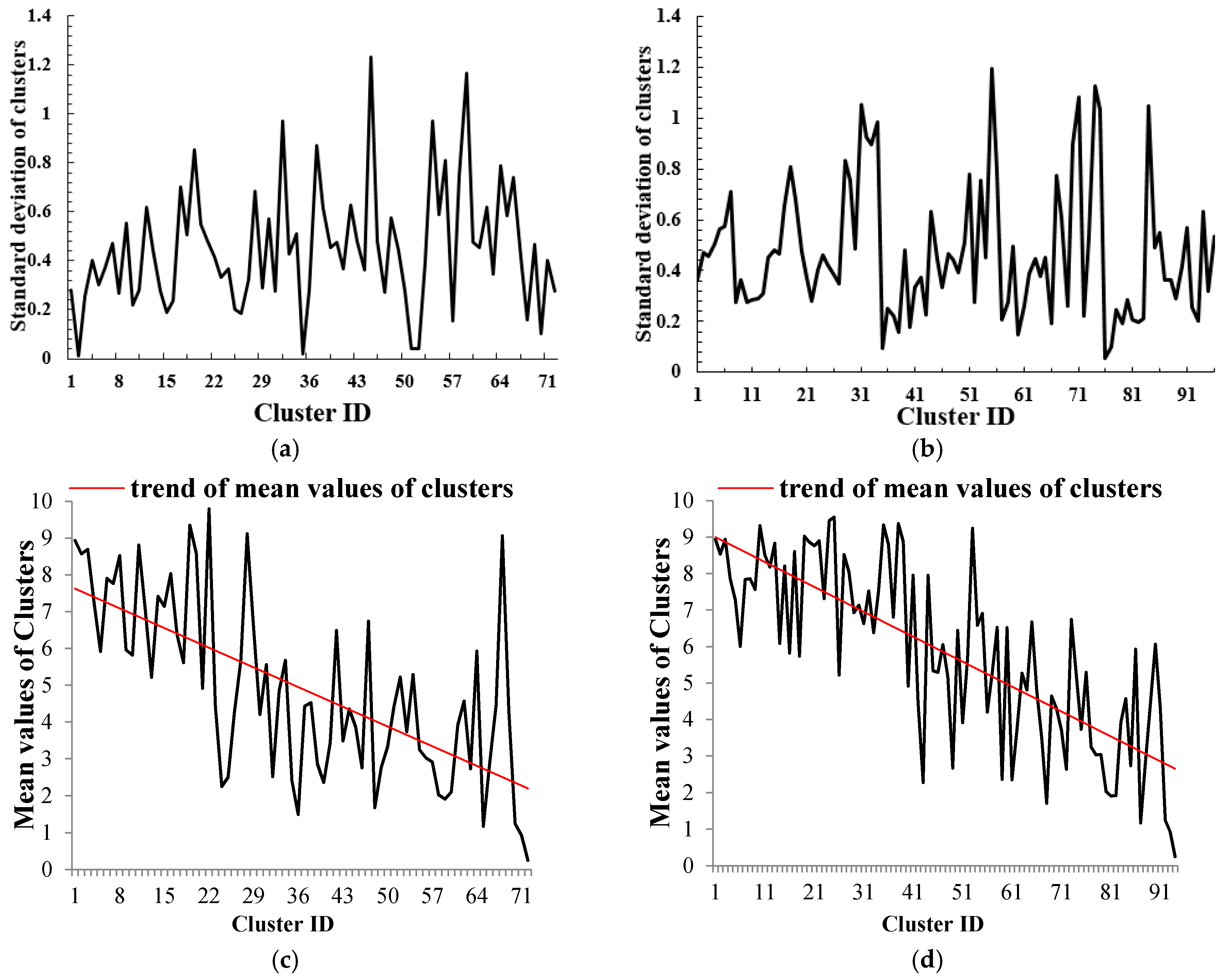
 represents the trend of mean values of clusters); (d) mean value of each cluster using DBSC ( represents the trend of mean values of clusters).
represents the trend of mean values of clusters); (d) mean value of each cluster using DBSC ( represents the trend of mean values of clusters).
represents the trend of mean values of clusters); (d) mean value of each cluster using DBSC ( represents the trend of mean values of clusters).


| Item | Variables | Factor | ||
|---|---|---|---|---|
| 1 | 2 | 3 | ||
| Thematic attributes | Land price | 0.728 | −0.556 | 0.202 |
| Distance from the nearest road | 0.627 | −0.683 | 0.019 | |
| Road network density | 0.736 | 0.650 | 0.098 | |
| Employment density | 0.908 | −0.114 | 0.006 | |
| Geometrical attributes | Aggregation degree | 0.694 | 0.686 | 0.140 |
| Area | −0.183 | 0.095 | 0.976 | |
| Our Method | DBSC Algorithm | |
|---|---|---|
| Number of Clusters | 72 | 95 |
| Number of Noise Points | 26 | 54 |
| CV value of mean values of clusters | 0.50 | 0.46 |
| City Centre | Algorithm | Precision | Recall | F1-Score |
|---|---|---|---|---|
| Wen Changge | Our method | 0.8053 | 0.8395 | 0.8219 |
| DBRS | 0.9606 | 0.3837 | 0.5484 | |
| He Dong | Our method | 0.4819 | 0.9756 | 0.6438 |
| DBRS | 0.9973 | 0.2587 | 0.4111 |
| Algorithm | Precision | Recall | F1-Score |
|---|---|---|---|
| Our method | 0.4130 | 0.9744 | 0.5801 |
| DBRS | 0.3220 | 0.9590 | 0.4821 |
© 2017 by the authors. Licensee MDPI, Basel, Switzerland. This article is an open access article distributed under the terms and conditions of the Creative Commons Attribution (CC BY) license (http://creativecommons.org/licenses/by/4.0/).
Share and Cite
Zhu, J.; Sun, Y. Building an Urban Spatial Structure from Urban Land Use Data: An Example Using Automated Recognition of the City Centre. ISPRS Int. J. Geo-Inf. 2017, 6, 122. https://0-doi-org.brum.beds.ac.uk/10.3390/ijgi6040122
Zhu J, Sun Y. Building an Urban Spatial Structure from Urban Land Use Data: An Example Using Automated Recognition of the City Centre. ISPRS International Journal of Geo-Information. 2017; 6(4):122. https://0-doi-org.brum.beds.ac.uk/10.3390/ijgi6040122
Chicago/Turabian StyleZhu, Jie, and Yizhong Sun. 2017. "Building an Urban Spatial Structure from Urban Land Use Data: An Example Using Automated Recognition of the City Centre" ISPRS International Journal of Geo-Information 6, no. 4: 122. https://0-doi-org.brum.beds.ac.uk/10.3390/ijgi6040122