
An Effective High-Performance Multiway Spatial Join Algorithm with Spark


1
Institute of Geographic Information Science, School of Earth Sciences, Zhejiang University, Hangzhou 310027, China
2
Department of Geography, Kent State University, Kent, OH 44240, USA
*
Author to whom correspondence should be addressed.
ISPRS Int. J. Geo-Inf. 2017, 6(4), 96; https://0-doi-org.brum.beds.ac.uk/10.3390/ijgi6040096
Submission received: 29 December 2016
/
Revised: 10 March 2017
/
Accepted: 22 March 2017
/
Published: 26 March 2017
Abstract
:Multiway spatial join plays an important role in GIS (Geographic Information Systems) and their applications. With the increase in spatial data volumes, the performance of multiway spatial join has encountered a computation bottleneck in the context of big data. Parallel or distributed computing platforms, such as MapReduce and Spark, are promising for resolving the intensive computing issue. Previous approaches have focused on developing single-threaded join algorithms as an optimizing and partition strategy for parallel computing. In this paper, we present an effective high-performance multiway spatial join algorithm with Spark (MSJS) to overcome the multiway spatial join bottleneck. MSJS handles the problem through cascaded pairwise join. Using the power of Spark, the formerly inefficient cascaded pairwise spatial join is transformed into a high-performance approach. Experiments using massive real-world data sets prove that MSJS outperforms existing parallel approaches of multiway spatial join that have been described in the literature.
1. Introduction
Spatial analysis is the core engine that drives research and applications of GIS. It can be used to explore spatial patterns and trends that might otherwise be difficult to detect [1]. Spatial join is a fundamental function of spatial analysis. It connects apparently unrelated data through spatial relationships and can facilitate data fusion. Early studies of how to improve the efficiency of spatial join were focused on the optimization of the algorithms. The PBSM algorithm partitions the inputs into manageable chunks and then joins them using a computational, geometry-based, plane-sweeping technique [2]. In [3], the author presents a scalable sweeping-based spatial join algorithm that achieves both efficiency with real-life data and robustness against highly skewed and worst-case datasets. TOUCH, a novel in-memory spatial join algorithm, uses hierarchical data-oriented space partitioning to permit a small memory footprint and a low number of comparisons [4]. To improve computational efficiency, cloud technologies are emerging as a new solution. The first spatial join algorithm with MapReduce is provided in [5]. Eldawy and Mokbel present a MapReduce-based spatial join method built in Spatial Hadoop, which is a MapReduce extension to Apache Hadoop that was designed specifically for spatial data [6]. In addition, with the development of efficient distributed memory computing platforms such as Spark, research has begun to focus on increasing the efficiency of spatial join queries with the help of Apache Spark [7,8,9,10].
Multiway spatial join is an extension of spatial join with multiple-inputs [11]. For example, the spatial query of “finding all the forests crossed by a river in each state” is a typical example of a multiway spatial join, which analyzes spatial relations among “forests”, “rivers” and “states” using “cross” and “within”. Similar examples are common in many other GIS applications. With the increase in spatial data volumes, the performance of multiway spatial join meets a bottleneck challenge in the context of big data [12]. How to solve the bottleneck challenge is an important research task for distributed spatial analysis [13].
The past two decades have witnessed many efforts to optimize both pairwise or two-way spatial join [2,3,4,14] and multiway spatial join [11,15,16,17,18,19,20]. Parallelized spatial join algorithms have been proposed to improve the performance of spatial joins [21,22,23,24]. Recently, the most popular high-performance computing framework, MapReduce [25], has received considerable attention in this field. Many pairwise spatial join approaches [5,6,26] have been implemented on the MapReduce platform. However, few studies have investigated the processing of multiway spatial joins in parallel. Recently, Gupta et al. [12] proposed an effective multiway spatial join algorithm called Controlled-Replicate on the MapReduce platform. Compared with a naïve All-Replicate method, the Controlled-Replicate method replicates a much smaller number of rectangles, thereby incurring a much lower communication cost among cluster nodes. Compared with another naïve two-way cascade method, the Controlled-Replicate method avoids processing large intermediate join results by processing them as a sequence of two map-reduce cycles, thereby incurring much lower reading and writing costs. Although the Controlled-Replicate method minimizes communication by exploiting the spatial locations of the rectangles, it requires two map-reduce cycles, and there is a trade-off in communication cost between the two map-reduce cycles. By increasing the communication in the first cycle by a small amount, communication in the second map-reduce cycle can be greatly reduced. Based on this trade-off principle, Gupta et al. [27] improved the Controlled-Replicate method by reducing the replicates and communication cost among cluster nodes. By importing a variable called ϵ to expend partitions and allocate more entities to each reducer, the replicates are fewer than those in the Controlled-Replicate method, which decreases the communication cost. However, regardless of the number of replicates, a round of two MapReduce jobs involves huge reading and writing costs. As a result, the intermediate results cannot be utilized immediately.
In this paper, we investigate the issue of paralleling multiway spatial join on the Spark framework [28]. The most significant characteristics of Spark in comparison with MapReduce are Spark’s support of iterative computation on the same data and its capability of efficient leveraging of distributed in-memory computation for fast large-scale data processing. Spark uses Resilient Distributed Datasets (RDDs) [29] to restore the persistent datasets on disk in order to distribute main memory and provide a series of “transformations” and “actions” to simplify parallel programming. These capabilities have prompted researchers to perform pairwise spatial join on Spark to achieve a high level of performance [30,31]. However, no studies have investigated in-memory computing for multiway spatial join, especially in parallelized or distributed platforms such as Spark.
In this article, we propose an effective multiway spatial join method with Spark (MSJS). MSJS realizes a natural solution of multiway spatial join via cascaded pairwise join, which means that the whole query problem is decomposed into a series of pairwise spatial joins. Excessive amounts of intermediate results have been proven to be the bottleneck of a cascaded pairwise join, especially on the MapReduce framework, due to the high communication cost and disk I/O (Input and Output) cost. By making full use of the in-memory iterative computation characteristics of Spark, MSJS is able to improve a cascaded pairwise join and achieve better performance by caching the intermediate results in memory. MSJS uses an efficient fixed uniform grid to partition the datasets. It then executes a pairwise cascade join via a cycle of in-memory operations (partition join, nested-loop join, merge, and repartition). Since the cascaded join reduces the datasets one by one, the whole algorithm resembles a “global” multiway index nested-loop join [18] in which the processes are in-memory distributed. The results of several experiments on massive real data have proved that MSJS outperforms existing parallel approaches for multiway spatial join with MapReduce.
The main contributions of this paper are as follows:
- We propose MSJS, an effective scalable and distributed multiway spatial join algorithm with Spark, which shows better performance in experiments than previous approaches that use MapReduce.
- We demonstrate how to take advantage of the in-memory iterative computing capabilities of Spark to bring the inefficient pairwise cascade multiway spatial join to a high performance level.
- We reveal that there is a linear relationship between the execution time of MSJS and the input data volume.
2. Background and Related Work
The pairwise spatial join algorithm is widely used in many GIS applications. The algorithm is aimed at finding pairs of objects from two spatial datasets that have spatial relationships that satisfy a specified spatial predicate. Various approaches of pairwise spatial join have been extensively researched [2,3,4,14,32]. These approaches can be summarized into two categories: approaches to develop the optimization algorithms for the single-threaded spatial join [4,14] and approaches to improve the performance of parallelized or distributed spatial join [21,24]. The approaches to optimize the single-threaded spatial join focus on two basic steps of spatial join: filter and refinement. Many classical methods have been proposed to reduce the candidate set by a filter step via sorting or indexing one or more datasets [3,14,21]. Some technologies have been developed to add a compute-intensive refinement step to further improve the performance [23].
Parallelization is an effective way to improve the performance of spatial join. Early parallel spatial join methods focused on fine-grained parallel computing, creating a parallel spatial index, and traversing the index synchronously to perform spatial join [21]. Zhou et al. [22] proposed the first parallel spatial join method based on a grid partition. Patel and DeWitt evaluated many partition-based parallel spatial join algorithms for querying databases, and they recommend clone join and shadow join [24], which are widely used in recent spatial join technologies. However, few methods have applied parallel technology to multiple input cases. Modern popular distributed computing frameworks such as MapReduce and Spark hold great promise for improving the performance of spatial join. Several studies have been conducted to improve the performance of pairwise spatial join on these platforms [5,6,26].
Multiway spatial joins, as complex forms of pairwise spatial joins, have been studied for almost two decades. One natural solution of a multiway spatial join is to decompose the join problem into a series of pairwise joins and then execute the pairwise joins one by one. In many cases, this approach results in poor performance. Papadias et al. proposed several methods to approach multiway spatial joins [11,16,18,19,20,33]. Their studies show that multiway spatial joins can be processed best by combining synchronous traversal with a pairwise method such as a plane-sweep or an index nested-loop algorithm [32].
Recently, a few studies have been conducted to investigate optimizing multiway spatial join on the MapReduce platform. Gupta et al. developed a Controlled-Replicate framework coupled with the project-split-replicate notation to handle multiway spatial join queries [12]. Controlled-Replicate runs as a cycle of two MapReduce jobs. The first job splits the objects by a fixed grid, allocates them in the same partition to a reducer and then marks the ones that satisfy the conditions of Controlled-Replicate. The second job replicates the marked objects to reducers by a replicate function and then processes the multiway spatial join in-memory. A specific strategy is employed to avoid duplicates. The experiments of Gupta et al. show that Controlled-Replicate outperforms the cascaded pairwise and all-replicates method on MapReduce.
Furthermore, Gupta et al. present an ϵ-Controlled-Replicate algorithm that improves on their previous work via reducing communication costs [27]. In contrast to the earlier Controlled-Replicate method, the ϵ-Controlled-Replicate algorithm uses more accurate conditions to mark the replicated objects. Therefore, the replicate number is much smaller, which can significantly improve performance. However, both Controlled-Replicate and ϵ-Controlled-Replicate execute two MapReduce jobs. Regardless of the number of marked objects, the input datasets must be read twice and the intermediate results must be written to disk and then reread. These processes require large amounts of disk I/O.
Hadoop-GIS [34] employed a different multiway spatial join method. The multiway spatial join method mainly focuses on star and clique joins. The query pipeline and the algorithm for processing multiway spatial joins are very similar to the two-way spatial join algorithm. Specifically, Hadoop-GIS extended the two-way spatial join algorithm to process multiway spatial join queries. Therefore, performance may still be poor due to the large amounts of disk I/O required in the MapReduce framework.
We propose MSJS, which can overcome the problems mentioned above. To our knowledge, no previous studies have proposed a Spark-based multiway spatial join method. In MSJS, the problem is converted into a series of pairwise spatial joins. Taking advantage of the in-memory iterative computation characteristics of Spark, MSJS can avoid the communication cost encountered by Hadoop-based approaches. In addition, MSJS involves a workflow of cascaded pairwise joins in which data redundancy does not increase with the number of join ways.
3. Methodology
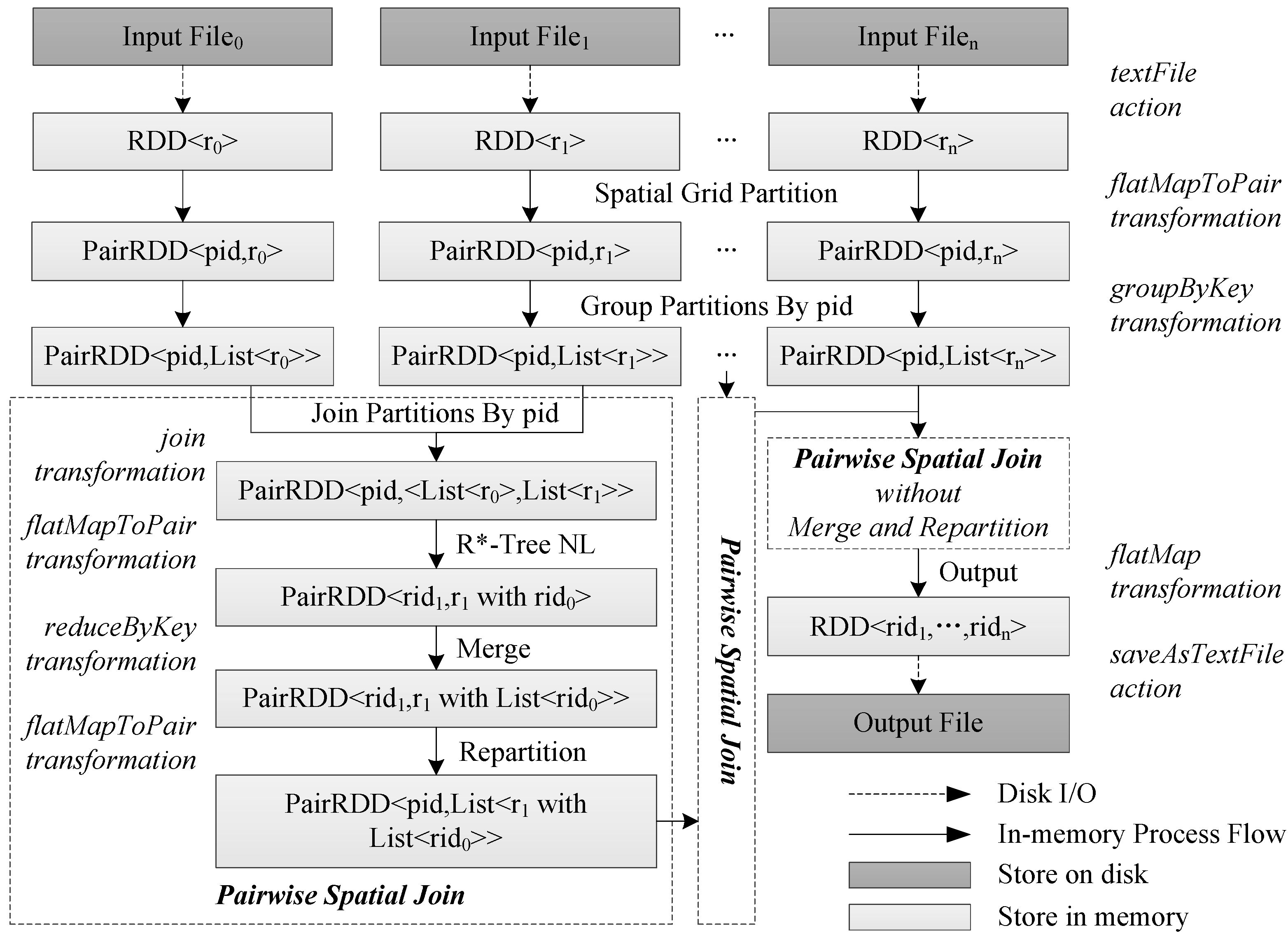
MSJS first partitions each dataset using a uniform grid. It then joins the partitions with the same IDs and executes the pairwise spatial joins in cascade. Using Spark, the intermediate results are cached in memory for iteratively computing. As the number of input datasets decreases, the execution speed of the computing processes increases. The R*-tree spatial index [35] is taken to optimize the pairwise spatial joins; in this way, the overall framework of MSJS is similar to the multiway index nested-loop join [18].
The flow diagram of the MSJS algorithm is shown in Figure 1.
The major phases of MSJS are summarized as follows:
Phase 1. Partition phase. Calculate the partition number of the uniform grid for each spatial object in parallel.
Phase 2. Group partition phase. Group the objects with the same partition ID from each dataset.
Phase 3. Cascaded pairwise join phase. Decompose the multiway spatial joins into a series of 2-way spatial joins. Then, process them one by one in memory with Spark.
Unlike the naïve approaches discussed in [12], the cascaded pairwise spatial join in MSJS is efficient mainly because the disk I/O in Spark is much smaller than that in MapReduce. The series of pairwise spatial joins in MSJS do not perform as a number of map and reduce tasks but rather as a series of transactions in Spark that are executed in memory.
3.1. Partition Phase
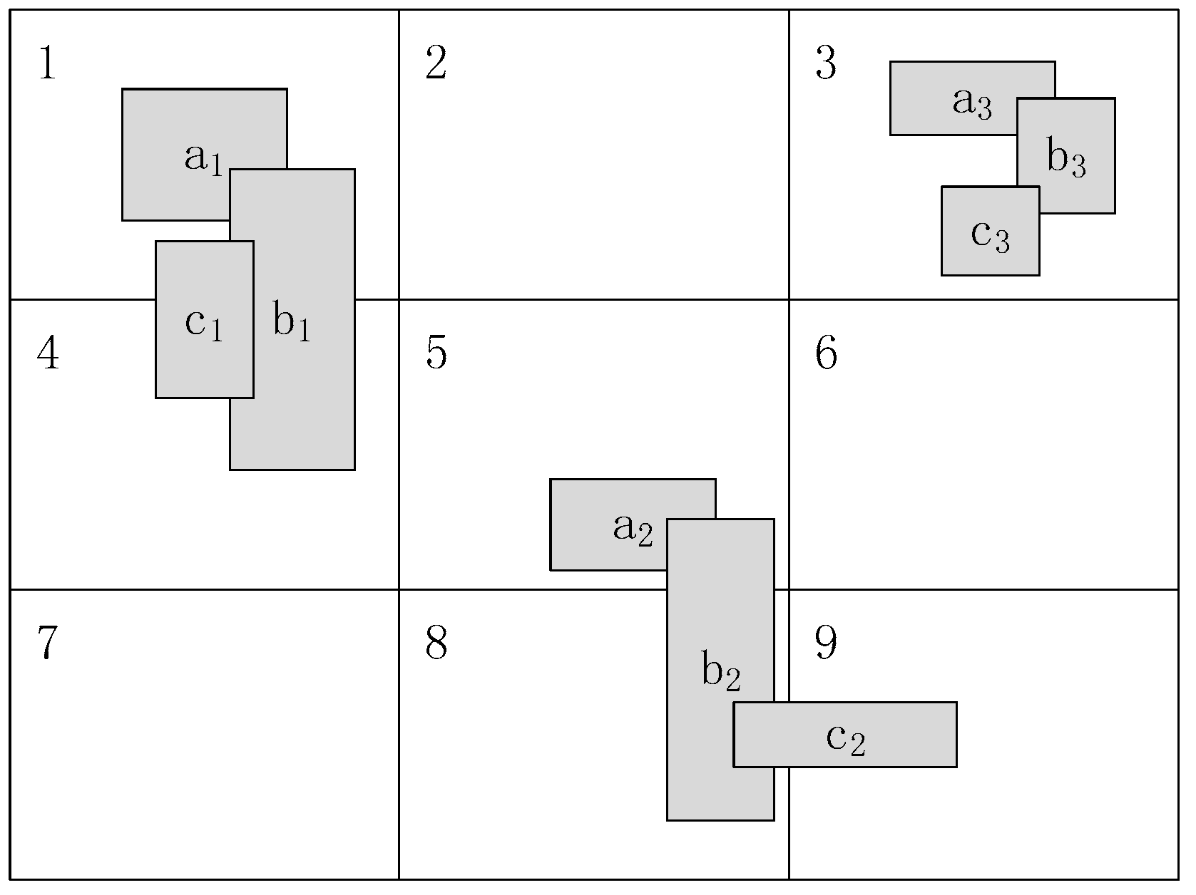
The goal of spatial partition is to reduce the data volume to fit the available memory and perform coarse-grained parallel computing (bulk computing). In two-way spatial join, a spatial object needs to be partitioned only into the grids it overlaps. However, in multiway spatial join, the same method cannot be applied. An example is provided in Figure 2, in which grid tiles 1–9 represent the uniform grids. Supposing there are three relation datasets (A, B and C) in the domain, we specify the spatial query as A overlaps B, and B overlaps C. The spatial objects are partitioned into the tiles overlapping with their Minimum Bounding Rectangles (MBRs). Of course, the tuples {a2, b2, c2} are one of the outputs, but none of the partitions will receive all of them; thus, none of the partitions can handle the multiway join of the tuples.
As discussed in [12], one way to solve this problem is to use the All-Replicate method, which means that all objects will be partitioned into their right and below grids (e.g., object a2 will be partitioned into grids 5, 6, 8 and 9). This ensures that at least one partition (partition 9) will receive the entire output tuples. Obviously, this method is naïve because it requires too many replicates and may have high communication costs between work nodes during computation. Both the Controlled-Replicate and ϵ-Controlled-Replicate methods offer ways to reduce the number of replicates. However, for in-memory frameworks such as Spark, the storage and calculation of the dataset occur in memory. Therefore, regardless of the number of replicates, the aforementioned replicate strategy may occupy a large memory space, which may lead to memory overflows.
To overcome this problem, MSJS takes into consideration the cascaded pairwise spatial joins, which are fitted for iterative in-memory computation frameworks such as Spark. In the pairwise join case, we need only to partition the datasets as aforementioned. The “textFile” action is conducted in Spark to read the files to RDDs that are stored on the distributed main memory for the datasets stored on the distributed file systems. Next, the “flatMapToPair” transformation, shown in Algorithm 1, performs the spatial partition. Each flatmap calculates the grid tiles overlapping with the objects’ MBR. Finally, the spatial partition phase returns the pairs of partition IDs and the geometries of each spatial object.
| Algorithm 1: Spatial Partitioning |
| PairRDD<Partition ID, Geometry>RDD<Geometry>.flatMapToPair (SpatialPartition) |
| Input: line: each line of spatial dataset file |
| Output: R: partitioned objects |
| Function SpatialPartition (line) |
| 1 |
| 2 |
| 3 |
| 4 |
| 5 |
| 6 |
3.2. Partition Group Phase
As discussed above, the outputs of the partition phase are spatial objects with their partition IDs. Some objects may have one or more partition IDs. To join the datasets in the corresponding partition, we need to merge the objects with the same partition IDs into one group. In Spark, we use a simple “GroupByKey” transformation to group the partitions; then, the objects in the same partition are merged into a list.
3.3. Cascaded Pairwise Join Phase
This phase processes a multiway join query as a series of pairwise joins. Each pairwise join (excluding the last one) is executed using the following four steps:
- 1
- Join the datasets that have the same partition ID.
- 2
- Perform the R*-tree index nested-loop join, which includes both the filter and refinement steps for the pairwise input datasets.
- 3
- Reduce the outputs of the first step by grouping the objects’ IDs of the datasets that will be joined next. The objects’ IDs already in the joined dataset are merged into a list.
- 4
- Repartition the outputs of the second step to prepare for the next cycle until termination.
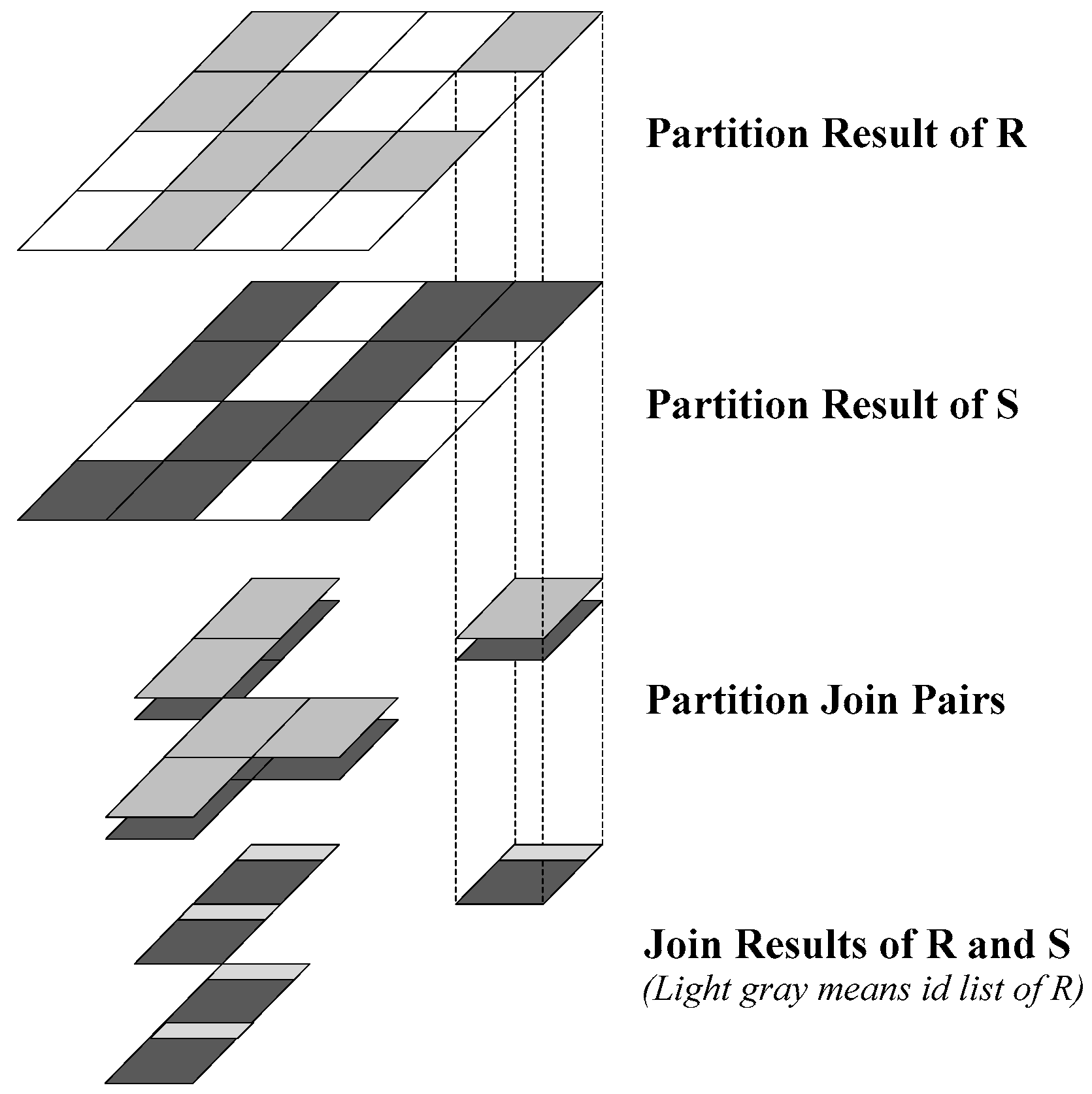
We denote the datasets of each pairwise input as R and S, where S represents the dataset that will be joined next. First, we join both partitioned datasets with the same partition IDs using Spark’s built-in “join” transformation. As shown in Figure 3, the first and second layers represent the partitions of datasets R and S. A gray tile means that the partition contains at least one spatial object, whereas a white tile means there are no spatial objects inside the partition. The results of the partition join are shown in the third layer in Figure 3. The operation works only on the corresponding partitions that are gray in both the R partition and the S partition. Partitions with only one or no gray tile are removed from main memory. Using this approach, MSJS can decrease more disk I/O in the partition phase than other spatial join techniques with MapReduce [6,26]. The fourth layer in Figure 3 represents the joined results of R and S. S will be cached in memory in its entirety, but only the IDs of the objects in R will be merged and stored in a list for each object in S.
Since all spatial entities have been cached to the RDD, MSJS can process the filter and refinement steps of spatial join synchronously. In addition, the traditional random access of data entity in the refinement stage, which may lead to high disk I/O costs, is omitted. R*-tree index is used in MSJS to decrease the duration of the nested-loop join in the filter and refinement steps. We do not review the R*-tree index nested-loop join here, as this index is well known. The duplicates in the corresponding partitions are eliminated using the reference point method [36] in the loop. For each output pair, MSJS holds the objects in S in memory while retaining only the IDs of the objects in R.
In the next step, the output pairs are further reduced by merging the objects’ IDs in S and the objects’ IDs in R into a combined list. Subsequently, the reduced datasets are repartitioned within the same grid as discussed in Section 3.1, and the next pairwise join cycle is initiated until all datasets and relations are computed. Finally, in the processing of the last pairwise spatial join, all merged IDs in the combined list are processed via a nested loop to generate the final results.
4. Experimental Evaluation
We conducted several experiments to measure the impact of cluster scale, partition number and dataset characteristics on MSJS’s performance. Under the same computing environment, we compared MSJS with three spatial join algorithms designed for MapReduce: Cascaded pairwise on Hadoop (HADOOP-CAS), Controlled-Replicate on Hadoop (HADOOP-CP) and ϵ-Controlled-Replicate on Hadoop (HADOOP-ϵCP) [12,27].
4.1. Experimental Setup and Datasets
The experiments were performed with Hadoop 2.6.0 and Spark 2.0.1 running on JDK 1.7 on DELL Power Edge R720 Servers. Each server was provisioned with one Intel Xeon E5-2630 v2 2.60 GHz processor, 32 GB main memory, a 500 GB SAS disk, a SUSE Linux enterprise server 11 SP2 operating system and the ext3 file system.
Table 1 shows the TIGER datasets used in these experiments. All files are in “csv” format and can be downloaded from the SpatialHadoop website [37].
We implemented MSJS on a Hadoop cluster and conducted the experiments on the Hadoop YARN (MapReduce’s next generation). In Spark’s YARN mode, the term “executor” refers to the tasks in progress on the nodes, “executor cores” refers to the task threads per executor, and “executor memory” refers to the maximum main memory allocated in each executor. All these parameters were preset before submitting a Spark job.
4.2. Impacts of Node and Thread Number
To evaluate the impacts of the numbers of nodes and threads on the performance of MSJS, we used “LM (arealandmark) overlaps with AW (areawater) and LW (linearwater)” as the query example. The number of partitions in this experiment was set to 200 × 400, the number of executor cores varied from 1 to 8, the number of executors varied from 1 to 4, and executor memory was set to 4 GB.
Table 2 shows the impacts of node number and threads per node on the performance of MSJS. There is a direct relationship between MSJS’s performance and the number of nodes when the number of threads per node is fixed; specifically, the performance of MSJS increases significantly as the number of nodes increases. This indicates that MSJS has high scalability. However, as the number of threads per node increases, MSJS’s execution time first improves and then degrades. Moreover, MSJS reaches its peak performance at 4 threads per node (the same as the number of Central Processing Unit, CPU cores). Because both data storage and data computing occupy large amounts of memory in Spark, an insufficient memory condition may degrade performance or cause execution to terminate.
4.3. Impact of Partition Number
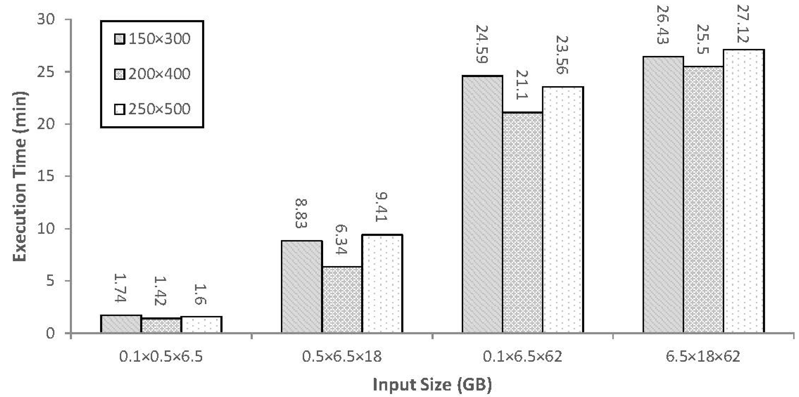
To evaluate the impact of the number of partitions on the performance of MSJS, we varied the input dataset sizes from 0.1 × 0.5 × 6.5 GB to 6.5 × 18 × 62 GB. We set the number of nodes, number of executors, number of executor cores, and amount of executor memory to 4, 4, 4, and 4 GB, respectively.
As shown in Figure 4, when the number of partitions is small, there is a large amount of data in each partition. This may trigger memory overflows or increase computation time. As the number of partitions increases, an excessive number of duplicates will lead to unnecessary calculation. Therefore, the most suitable partition is one in which the number of grids is 200 × 400; this partition performs better than the others. However, as the input size varies, the most suitable number of partitions may change as well. As shown in Figure 4, when the input size is either small or large, the performance differences among different numbers of partitions are very small. Therefore, using an overly large number of partitions or all of the partitions may not be appropriate in these cases.
Choosing an accurate and optimal number of grids is difficult because of the volume differences among the original datasets. The most commonly used method is to set the number as a parameter, with the minimum number of grids determined by several factors such as the number of computing nodes and the memory limit in each node. It is important to ensure that each node in the calculation does not exceed the memory limit.
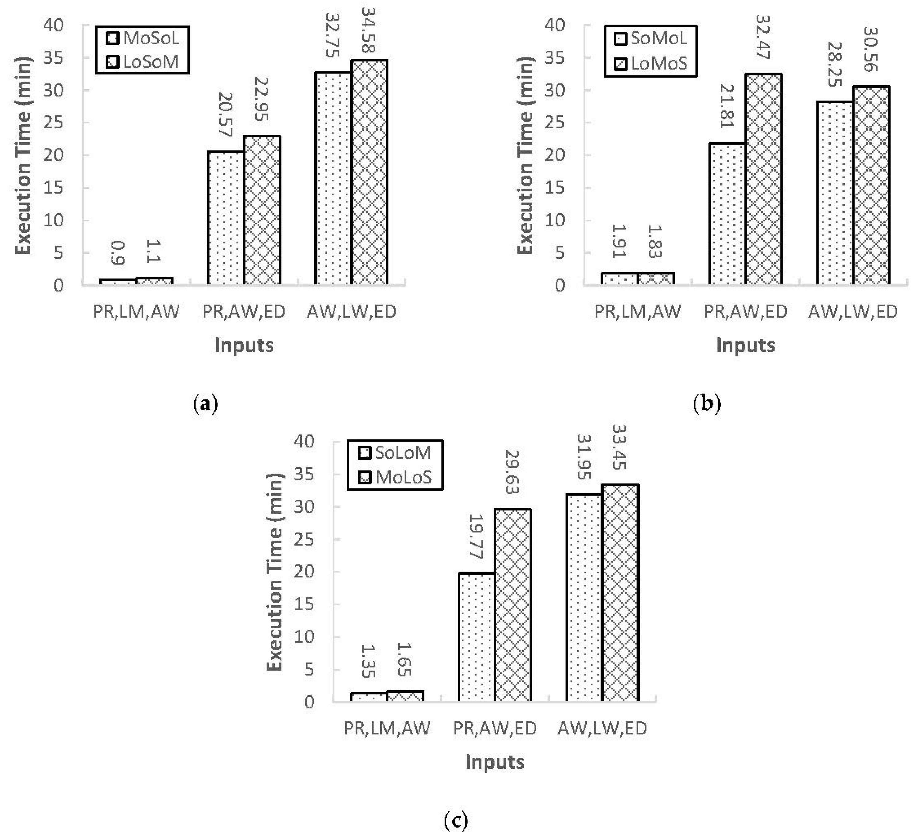
4.4. Impact of Input Sequence
To evaluate the impact of the input sequence on the performance of MSJS, we use three input groups (PR, LM, and AW; PR, AW, and ED; and AW, LW, and ED) to vary the input sequence for MSJS. Again, we set the number of nodes, number of executors, number of executor cores, and amount of executor memory to 4, 4, 4, and 4 GB, respectively. The grid size was 200 × 400.
As shown in Figure 5, different input sequences may lead to different performance for the same multiway spatial join query. For example, MoSoL and LoSoM in Figure 5a are the same multiway spatial join query with a different input sequence. As shown in Figure 5a, when the intermediate input datasets are small, both MoS and SoM are processed rapidly; thus, the performance is only slightly affected by input sequence. However, as shown in Figure 5b,c, when the intermediate input datasets are large, performance is significantly affected by input sequence, especially when the size of inputs has disparity. This is mainly because for pairwise spatial join with Spark, when one dataset is small (e.g., dataset PR), the performance of spatial partition, partition join and local join is efficient. Thus, when the two small datasets are joined first, both two rounds of MSJS are small-to-large spatial joins, which will be efficient for the aforementioned reasons. However, when the smaller dataset is not sufficiently small (e.g., dataset AW), the performance will be poor, as both rounds of MSJS may take a long time to be executed. From the results of these experiments, we conclude that an efficient way to optimize MSJS is to adjust the input sequence such that smaller datasets are joined first.
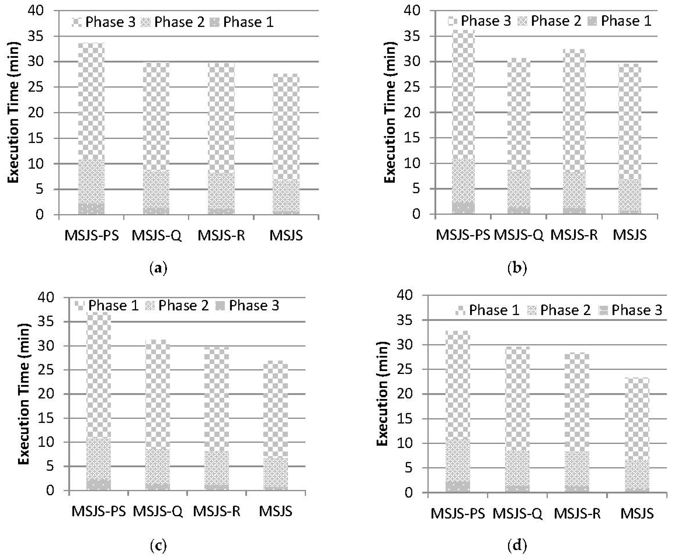
4.5. Impacts of Different Spatial Predicates and In-Memory Join Algorithms
To evaluate the impacts of the different spatial predicates and in-memory join algorithms on the performance of MSJS, we used AW, LW, and ED as the input datasets for the experiments and recorded the execution time of each phase in MSJS. In addition to the default R*-tree indexed nested-loop join (MSJS), three other in-memory join algorithms designed for refinement stage of spatial join in MSJS were compared: the plane-sweep (MSJS-PS), quadtree index nested-loop join (MSJS-Q), and R-tree indexed nested-loop join (MSJS-R). We set the number of nodes, number of executors, number of executor cores, and amount of executor memory to 4, 4, 4, and 6 GB, respectively.
From Figure 6a–d, it can be seen that the default R*-tree indexed nested-loop join has the best performance for all spatial predicates. As the complexity of the four topological analyses of refinement stage of in-memory is different, for the same in-memory join algorithm, the query “AW contains LW and LW contains ED” always outperforms the query “AW touches LW and LW touches ED”.
Regarding the execution time in each phase, phase 1 is consistently the least time-consuming part. This is because phase 1 involves only calculating the partition number for each spatial object in parallel, the process has a linear computing complexity and there is no communication cost among tasks. The execution time of phase 2 is between the times of phase 1 and 3. This phase groups the objects that have the same partition together; because the objects are scattered on different nodes, a shuffle process is required to collect them, which results in network communication. The execution times of phase 1 and phase 2 are related to only the volume of the dataset; therefore, they are approximately equal in the experiments that process the same datasets. Since phase 3 contains a loop of pairwise join and a repartition process is involved in each round of the loop, this phase typically takes the most time.
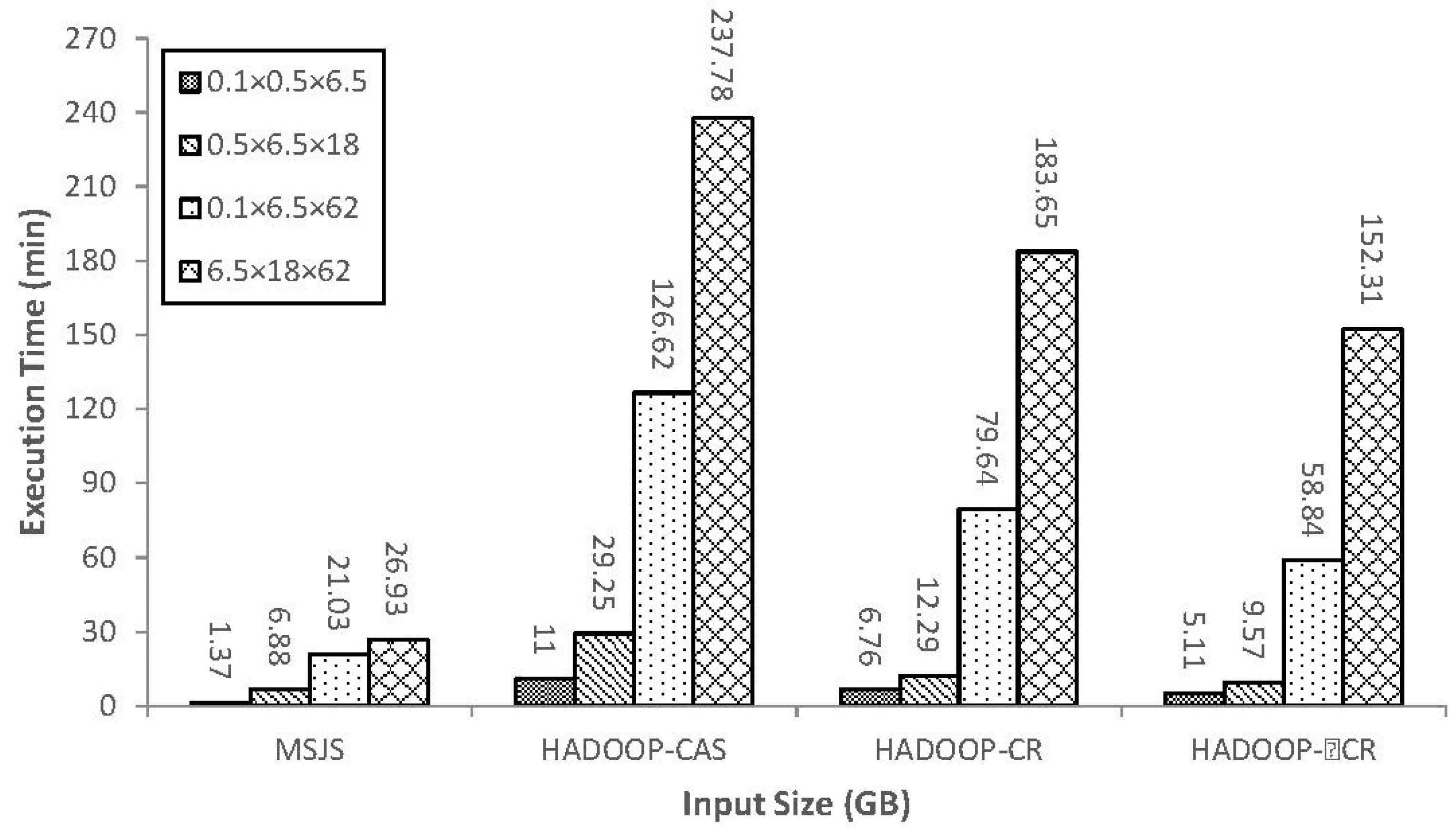
4.6. Comparison of HADOOP-CAS, HADOOP-CP, HADOOP-ϵCP and MSJS
Using the differently sized datasets listed above as inputs, we made several comparison tests with other spatial join algorithms designed for MapReduce, such as cascaded pairwise on Hadoop (HADOOP-CAS), Controlled-Replicate on Hadoop (HADOOP-CP), and ϵ-Controlled-Replicate on Hadoop (HADOOP-ϵCP). For MSJS, we used 4 executors and 4 executor cores. We set executor memory to 6 GB and the number of partitions to 200 × 400. All tests were run on the same cluster with the corresponding software frameworks.
We varied the input dataset sizes from 0.1 × 0.5 × 6.5 GB to 6.5 × 18 × 62 GB. Figure 7 shows the comparison results of MSJS with HADOOP-CAS, HADOOP-CP, and HADOOP-ϵCP. The performance of MSJS is obviously much better than the performance of the others. The main limitations of the three Hadoop-based algorithms are the high communication and I/O costs in the complex computing flow, which are caused by not only the Hadoop framework but also the huge amount of duplicates during computation. MSJS reduces the size of datasets by merging the duplicates during cascaded pairwise spatial join, and it makes full use of the iterative computing advantage of Spark. The results prove that MSJS can not only deal with massive spatial datasets but also perform more efficiently than other existing parallel spatial join algorithms reported in the literature.
5. Conclusions and Future Work
In this study, we propose a high-performance multiway spatial join algorithm with Spark, MSJS. MSJS can be deployed easily on large-scale cloud clusters. Our experimental results show that MSJS can significantly improve the performance of multiway spatial joins on massive spatial datasets. The iterative computation characteristics of Spark enable in-memory parallel cascaded pairwise spatial join with minimal disk-access costs. By taking advantage of the highly utilized space and the fast retrieving speed of the R*-tree, each partition executes the index nested-loop pairwise spatial joins with high performance. With extensive evaluations using real massive datasets, we demonstrated that MSJS outperforms other existing multiway spatial join approaches with MapReduce that have been reported in the literature. We plan to develop novel methods in the future to reduce the extra refinement processes that occur during the cascaded pairwise join phase to improve the performance.
Acknowledgments
This research was funded by National Natural Science Foundation of China (41471313, 41671391), Science and Technology Project of Zhejiang Province (2014C33G20), Public Science and Technology Research Funds Projects (2015418003), and the National Science Foundation (1416509, 1535031, 1637242).
Author Contributions
Zhenhong Du designed the study and drafted the manuscript; Xianwei Zhao extensively revised the manuscript and conducted computing experiements; Xinyue Ye improved the conceptual framework and participated in manuscript revision; Jingwei Zhou contributed to the study design and made improvements to the algorithm; Feng Zhang contributed to the experimental study; and Renyi Liu edited the manuscript. All authors have read and approved the final manuscript.
Conflicts of Interest
The authors declare no conflict of interest.
References
- Longley, P.A.; Goodchild, M.F.; Maguire, D.J.; Rhind, D.W. Geographic Information Science and Systems, 4th ed.; John Wiley & Sons: Chichester, UK, 2015; pp. 290–292. [Google Scholar]
- Patel, J.M.; DeWitt, D.J. Partition based spatial-merge join. In Proceedings of the 1996 ACM SIGMOD International Conference on Management of Data, Montreal, QC, Canada, 4–6 June 1996; ACM: New York, NY, USA, 1996; pp. 259–270. [Google Scholar]
- Arge, L.; Procopiuc, O.; Ramaswamy, S.; Suel, T.; Vitter, J.S. Scalable sweeping-based spatial join. In Proceedings of the 24th International Conference on Very Large Data Bases, New York, NY, USA, 24–27 August 1998; pp. 570–581. [Google Scholar]
- Nobari, S.; Tauheed, F.; Heinis, T.; Karras, P. TOUCH: In-memory spatial join by hierarchical data-oriented partitioning. In Proceedings of the 2013 ACM SIGMOD International Conference on Management of Data, New York, NY, USA, 22–27 June 2013; ACM: New York, NY, USA, 2013; pp. 701–712. [Google Scholar]
- Zhang, S.; Han, J.; Liu, Z.; Wang, K.; Xu, Z. SJMR: Parallelizing spatial join with MapReduce on clusters. In Proceedings of the 2009 IEEE International Conference on Cluster Computing and Workshops, New Orleans, LA, USA, 31 August–4 September 2009. [Google Scholar]
- Eldawy, A.; Mokbel, M.F. SpatialHadoop: A MapReduce framework for spatial data. In Proceedings of the International Conference on Data Engineering, Seoul, Korea, 13–17 April 2015; pp. 1352–1363. [Google Scholar]
- Xie, D.; Li, F.; Yao, B.; Li, G.; Zhou, L.; Guo, M. Simba: Efficient in-memory spatial analytics. In Proceedings of the ACM SIGMOD Conference, San Francisco, CA, USA, 26 June–1 July 2016; ACM: New York, NY, USA, 2016. [Google Scholar]
- Baig, F.; Mehrotra, M.; Vo, H.; Wang, F.; Saltz, J.; Kurc, T. SparkGIS: Efficient comparison and evaluation of algorithm results in tissue image analysis studies. In Biomedical DATA Management and Graph Online Querying; Springer: Cham, Switzerland, 2016; pp. 134–146. [Google Scholar]
- Yu, J.; Wu, J.; Sarwat, M. GeoSpark: A cluster computing framework for processing large-scale spatial data. In Proceedings of the ACM SIGSPATIAL International Conference on Advances in Geographic Information Systems, Seattle, WA, USA, 3–6 November 2015; ACM: New York, NY, USA, 2015. [Google Scholar]
- Zhang, F.; Zhou, J.; Liu, R.; Du, Z.; Ye, X. A new design of high-performance large-scale GIS computing at a finer spatial granularity: A case study of spatial join with spark for sustainability. Sustainability 2016, 8, 926. [Google Scholar] [CrossRef]
- Papadias, D.; Arkoumanis, D. Search algorithms for multiway spatial joins. Int. J. Geogr. Inf. Sci. 2002, 16, 613–639. [Google Scholar] [CrossRef]
- Gupta, H.; Chawda, B. Processing multi-way spatial joins on map-reduce. In Proceedings of the International Conference on Extending Database Technology, Genoa, Italy, 18–22 March 2013; pp. 113–124. [Google Scholar]
- Yang, C.; Goodchild, M.F.; Huang, Q.; Nebert, D.; Raskin, R.; Xu, Y.; Bambacus, M.; Fay, D. Spatial cloud computing: How Can the Geospatial sciences use and help shape cloud computing? Int. J. Digit. Earth 2011, 4, 305–329. [Google Scholar] [CrossRef]
- Vassilakopoulos, M.; Corral, A.; Karanikolas, N.N. Join-queries between two spatial datasets indexed by a Single R*-tree. Lect. Notes Comput. Sci. 2011, 6543, 533–544. [Google Scholar]
- Corral, A.; Manolopoulos, Y.; Theodoridis, Y.; Vassilakopoulos, M. Distance join queries of multiple inputs in spatial databases. In Advances in Databases and Information Systems; Kalinichenko, L., Manthey, R., Thalheim, B., Wloka, U., Eds.; Springer: Berlin, Germany, 2003; pp. 323–338. [Google Scholar]
- Papadias, D.; Mamoulis, N.; Delis, V. Algorithms for querying by spatial structure. In Proceedings of the 24th International Conference on Very Large Data Bases, New York, NY, USA, 27–27 August 1998; pp. 546–557. [Google Scholar]
- Park, H.; Cha, G.; Chung, C. Multi-way spatial joins using R-trees: Methodology and performance evaluation. In Proceedings of the 6th International Symposium on Advances in Spatial Databases, Hong Kong, China, 20–23 July 1999; pp. 229–250. [Google Scholar]
- Papadias, D.; Mamoulis, N.; Theodoridis, Y. Processing and optimization of Multiway spatial joins using R-trees. In Proceedings of the 18th ACM Sigmod-SIGACT-SIGART Symposium on Principles of Database Systems, Philadelphia, PA, USA, 31 May–3 June 1999; ACM: New York, NY, USA, 1999; pp. 44–55. [Google Scholar]
- Papadias, D.; Mamoulis, N.; Theodoridis, Y. Constraint-based processing of Multiway spatial joins. Algorithmica 2001, 30, 188–215. [Google Scholar] [CrossRef]
- Papadias, D.; Mamoulis, N.; Theodoridis, Y. Multiway spatial joins. ACM Trans. Database Syst. 2001, 30, 188–215. [Google Scholar]
- Brinkhoff, T.; Kriegel, H.P.; Seeger, B. Parallel processing of spatial joins using R-trees. In Proceedings of the 12th International Conference on Data Engineering, New Orleans, LA, USA, 26 February–1 March 1996; pp. 258–265. [Google Scholar]
- Zhou, X.; Abel, D.J.; Truffet, D. Data partitioning for parallel spatial join processing. Geoinformatica 1998, 2, 175–204. [Google Scholar] [CrossRef]
- Ray, S.; Simion, B.; Brown, A.D.; Johnson, R. Skew-resistant parallel in-memory spatial join. In Proceedings of the 26th International Conference on Scientific and Statistical Database, Aalborg, Denmark, 30 June–2 July 2014; ACM: New York, NY, USA, 2014. [Google Scholar]
- Patel, J.M.; DeWitt, D.J. Clone join and shadow join: Two parallel spatial join algorithms. In Proceedings of the 8th ACM International Symposium on Advances in Geographic Information Systems, Washington, DC, USA, 6–11 November 2000; pp. 54–61. [Google Scholar]
- Apache Hadoop. Available online: http://hadoop.apache.org (accessed on 30 June 2015).
- Aji, A.; Wang, F.; Vo, H.; Lee, R.; Liu, Q.; Zhang, X.; Saltz, J. Hadoop-GIS: A high performance spatial data warehousing system over MapReduce. Proc. VLDB Endow. 2013, 6, 1009–1020. [Google Scholar] [CrossRef]
- Gupta, H.; Chawda, B. ε-Controlled-Replicate: An improved Controlled-Replicate algorithm for multi-way spatial join processing on map-reduce. In Web Information Systems Engineering (WISE’14); Benatallah, B., Bestavros, A., Manolopoulos, Y., Vakali, A., Zhang, Y., Eds.; Springer: Berlin, Germany, 2014; pp. 278–293. [Google Scholar]
- Apache Spark. Available online: http://spark.apache.org (accessed on 30 June 2015).
- Zaharia, M.; Chowdhury, M.; Das, T.; Dave, A.; Ma, J.; McCauley, M.; Franklin, M.J.; Shenker, S.; Stoica, I. Resilient distributed datasets: A fault-tolerant abstraction for in-memory cluster computing. In Proceedings of the 9th USENIX Conference on Networked Systems Design and Implementation, San Jose, CA, USA, 25–27 April 2012; USENIX Association: Berkeley, CA, USA, 2012; p. 2. [Google Scholar]
- You, S.; Zhang, J.; Gruenwald, L. Large-scale spatial join query processing in cloud. In Proceedings of the International Workshop on Cloud Data Management, Seoul, Korea, 13–17 April 2015; pp. 34–41. [Google Scholar]
- You, S.; Zhang, J.; Gruenwald, L. Spatial join query processing in cloud: Analyzing design choices and performance comparisons. In Proceedings of the International Conference on Parallel Processing Workshops (ICPPW), Beijing, China, 1–4 September 2015; pp. 90–97. [Google Scholar]
- Jacox, E.H.; Samet, H. Spatial join techniques. ACM Trans. Database Syst. 2007, 32, 7. [Google Scholar] [CrossRef]
- Papadias, D.; Arkoumanis, D. Approximate processing of multiway spatial joins in very large databases. In Proceedings of the 8th International Conference on Extending Database Technology; Jensen, C.S., Šaltenis, S., Jeffery, K.G., Pokorny, J., Bertino, E., Böhn, K., Jarke, M., Eds.; Springer: Berlin, Germany, 2002; pp. 179–196. [Google Scholar]
- Aji, A. High Performance Spatial Query Processing for Large Scale Spatial Data Warehousing. Ph.D. Thesis, Laney Graduate School, Math and Computer Science, Emory University, Atlanta, GA, USA, 2014. [Google Scholar]
- Kriegel, H.; Kunath, P.; Renz, M. R*-Tree. In Encyclopedia of GIS; Shekhar, S., Xiong, H., Zhou, X., Eds.; Springer International Publishing: Cham, Switzerland, 2015; pp. 1–8. [Google Scholar]
- Dittrich, J.P.; Seeger, B. Data redundancy and duplicate detection in spatial join processing. In Proceedings of the 16th IEEE International Conference on Data Engineering, San Diego, CA, USA, 3 March 2000; pp. 535–546. [Google Scholar]
- SpatialHadoop. Available online: http://spatialhadoop.cs.umn.edu/datasets.html (accessed on 8 May 2015).
Figure 1.
Multiway spatial join with Spark (MSJS).

Figure 2.
Partitioning of spatial objects. Whereas a1, a2, a3, b3 and c3 are partitioned into tiles containing them, the others are partitioned into more than one tile, with which they overlap. Thus, only tile 1 and tile 3 receive the whole output tuples.
Figure 2.
Partitioning of spatial objects. Whereas a1, a2, a3, b3 and c3 are partitioned into tiles containing them, the others are partitioned into more than one tile, with which they overlap. Thus, only tile 1 and tile 3 receive the whole output tuples.

Figure 3.
One cycle of pairwise spatial partition join.

Figure 4.
Impact of the number of partitions.

Figure 5.
(a–c) Impact of input sequence. (S, M, and L refer to the small, medium, and large datasets of the inputs, respectively; o means the spatial predicate “overlaps”. For example, MoSoL on inputs of “PR, LM, AW” means that the multiway spatial join of LM (the medium dataset) overlaps with PR (the small dataset) and AW (the large dataset)).

Figure 6.
Impacts of different spatial predicates and in-memory join algorithms. (Each graph corresponds to a specific spatial predicate. (a), (c), (b) and (d) represent “overlaps”, ”touches”, ”disjoints” and “contains”, respectively.)
Figure 6.
Impacts of different spatial predicates and in-memory join algorithms. (Each graph corresponds to a specific spatial predicate. (a), (c), (b) and (d) represent “overlaps”, ”touches”, ”disjoints” and “contains”, respectively.)

Figure 7.
Performance comparison of MSJS with HADOOP-CAS, HADOOP-CP, and HADOOP-ϵCP.


Table 1.
The TIGER datasets.
| Dataset | Abbreviation | Records | Size |
|---|---|---|---|
| edges | ED | 72,729,686 Polygons | 62 GB |
| linearwater | LW | 5,857,442 Polylines | 18.3 GB |
| areawater | AW | 2,298,808 Polygons | 6.5 GB |
| arealandmark | LM | 121,960 Polygons | 406 MB |
| primaryroads | PR | 13,373 Polylines | 77 MB |
Table 2.
Impacts of node number and threads per node (min).
| Number of Nodes | ||||
|---|---|---|---|---|
| Threads per Node | 1 | 2 | 4 | |
| 1 | >60 | 27.68 | 23.38 | |
| 2 | - | 26.32 | 16.68 | |
| 4 | - | 18.65 | 15.42 | |
| 8 | - | - | 17.33 | |
© 2017 by the authors. Licensee MDPI, Basel, Switzerland. This article is an open access article distributed under the terms and conditions of the Creative Commons Attribution (CC BY) license (http://creativecommons.org/licenses/by/4.0/).
Share and Cite
MDPI and ACS Style
Du, Z.; Zhao, X.; Ye, X.; Zhou, J.; Zhang, F.; Liu, R. An Effective High-Performance Multiway Spatial Join Algorithm with Spark. ISPRS Int. J. Geo-Inf. 2017, 6, 96. https://0-doi-org.brum.beds.ac.uk/10.3390/ijgi6040096
AMA Style
Du Z, Zhao X, Ye X, Zhou J, Zhang F, Liu R. An Effective High-Performance Multiway Spatial Join Algorithm with Spark. ISPRS International Journal of Geo-Information. 2017; 6(4):96. https://0-doi-org.brum.beds.ac.uk/10.3390/ijgi6040096
Chicago/Turabian StyleDu, Zhenhong, Xianwei Zhao, Xinyue Ye, Jingwei Zhou, Feng Zhang, and Renyi Liu. 2017. "An Effective High-Performance Multiway Spatial Join Algorithm with Spark" ISPRS International Journal of Geo-Information 6, no. 4: 96. https://0-doi-org.brum.beds.ac.uk/10.3390/ijgi6040096
Note that from the first issue of 2016, this journal uses article numbers instead of page numbers. See further details here.