
A G-Super4PCS Registration Method for Photogrammetric and TLS Data in Geology


1
School of Earth Sciences and Engineering, Hohai University, Nanjing 210098, China
2
Engineering Research Center for Rock-Soil Drilling & Excavation and Protection, Ministry of Education, Wuhan 430074, China
3
Institute for Cartography, TU Dresden, Dresden 01062, Germany
*
Author to whom correspondence should be addressed.
ISPRS Int. J. Geo-Inf. 2017, 6(5), 129; https://0-doi-org.brum.beds.ac.uk/10.3390/ijgi6050129
Submission received: 27 March 2017
/
Revised: 18 April 2017
/
Accepted: 24 April 2017
/
Published: 28 April 2017
Abstract
:Photogrammetry and Terrestrial laser scanning (TLS) are the two primary non-contact active measurement techniques in geology. Integrating TLS data with digital images may achieve complementary advantages of spatial information as well as spectrum information, which would be very valuable for automatic rock surface extraction. In order to extract accurate and comprehensive geological information with both digital images and TLS point cloud, the registration problem for different sensor sources should be solved first. This paper presents a Generalized Super 4-points Congruent Sets (G-Super4PCS) algorithm to register the TLS point cloud as well as Structure from Motion (SfM) point cloud generated from disordered digital images. The G-Super4PCS algorithm mainly includes three stages: (1) key-scale rough estimation for point clouds; (2) extraction for the generalized super 4-points congruent base set and scale adaptive optimization; and (3) fine registration with Iterative Closest Point (ICP) algorithm. The developed method was tested with the columnar basalt data acquired in Guabushan National Geopark in Jiangsu Province, China. The results indicate that the proposed method could be used for indirect registration between digital images and TLS point cloud, and the result of which would be prepared for further integration research.
1. Introduction
Rock surface includes joints, fractures, faults and other geological structures; the properties of which govern the overall behavior of the rock masses. A detailed investigation aiming at the corresponding geological environment is necessary for a rock engineering research. The geometrical information, distribution and combination condition of the rock surface are the basis on which rock mass classification and engineering geological evaluation can proceed well. Therefore, it is vital for hydropower engineering, transportation engineering and mining engineering to extract rock surface accurately, efficiently and fully, which has important realistic significance for engineering exploration, design, evaluation and construction.
However, most basic engineering construction projects focus on alpine and gorge regions, which are so dangerous and inaccessible that the traditional contact measurements cannot proceed efficiently, safely, and quickly. Instead of the traditional contact measurements, the non-contact active measurements, mainly including close-range photogrammetry and TLS, could collect image or point cloud data and then finish rock surface extraction more conveniently and comprehensively in a virtual digital environment generated from these data.
Terrestrial laser scanning (TLS), emerging in the mid-1990s, allows capturing an accurate 3D model of an object in short time, which could be used for several purposes. TLS is an active and non-contact measurement technique, which can obtain the spatial coordinates of an object with high speed and accuracy by measuring the time-of-flight of laser signals [1]. High temporal resolution, high spatial resolution and uniform accuracy make the TLS data rather appropriate for many applications, including dangerous and inaccessible regions. However, TLS data are poor at expressing the object features due to characteristics such as unstructured 3D point clouds. Photogrammetric techniques processing stereoscopic images may be considered largely complementary to TLS, delivering RGB data plus possibly further spectral channel information. Thus, integrating the TLS data with digital image data may achieve complementary advantages of spatial information as well as spectrum information. This integration may be very valuable for geology research.
One crucial problem that the research of geological information extraction based on the integration of TLS data and image data involves is about the registration between point cloud and digital image. Because of the different sensor sources and reference systems, a spatial similarity transformation is essential to achieve registration. At present, many domestic and international scholars carried on a great deal of research on this, which can mainly be divided into four groups: (1) registration with the digital image and the intensity image generated by point cloud data; (2) registration with the point cloud data respectively acquired by TLS and generated by digital images; (3) registration through corresponding features extracted from both the TLS point cloud and the images; and (4) registration through artificial targets (e.g., retro-reflective targets). As each of the above methods has its pros and cons in certain application, it is important to find the tradeoff that is best suited for geology applications. Compared with the first two groups, the latter two implement the registration based on the original data sources, which effectively reduces error accumulation. However, for geological research objects, the irregular appearance and indeterminate distribution of rock surface make it difficult to directly extract corresponding primitives from the two data either by interactive methods or by automatic methods.
As a primary technique of computer vision to reconstruct 3D scene geometry and camera motion from a set of images of a static scene, Structure from Motion (SfM) has been applied in more and more areas, including geomorphology, medical science, archaeology and cultural heritage [2,3,4,5,6]. SfM has the potential to provide both a low cost and time efficient method for collecting data on the object surface [7]. SfM technique neither needs any prior knowledge about camera positions and orientation, nor targets with known 3D coordinates, all of which can be solved simultaneously using a highly redundant, iterative bundle adjustment procedure, based on a database of features automatically extracted from a set of multiple overlapping images [8,9]. Therefore, it seems more feasible to indirectly register digital images and TLS point cloud by use of the SfM point cloud from images and TLS point cloud.
Because of the complicated and irregular geological structure, it is difficult for registration to directly and automatically extract primitives from SfM point cloud and TLS point cloud, such as point-based, regular line segment-based and planar-based. In recent years, a novel 4-points congruent base has been proposed for 3D point clouds registration [10]. Instead of more than three corresponding points’ selection, these algorithms calculate the rigid transformation parameters by use of 4-points congruent base sets, the advantages of which could be concluded as follows: (1) There is no need to assume both the initial position and orientation of the two point clouds. (2) It is unnecessary to depend on any regular geometrical features from the research object itself. (3) The overlap between the two point clouds does not need to be known in advance. (4) It is robust to noise and outliers, thus it does not require preprocessing such as filtering or noise reduction. In consideration of all the above advantages, the registration theory of the 4-points congruent base is especially suitable for the geological objects. The existing algorithms, such as 4PCS and Super4PCS, are limited to those data sets from the same sensor. However, the geological data sources in this paper are r acquired by a digital camera and a terrestrial laser scanner, and with different scales. Therefore, to use 4-points congruent base sets for registration, the scales between the two point clouds should be unified first.
Based on all the above analysis, this paper presents a fully automated method, G-Super4PCS, for indirect registration of digital images and TLS point cloud data. This algorithm firstly takes the SfM and TLS key point clouds, respectively, extracted from digital images and the original TLS point cloud for rigid transformation parameters rough estimation, and then takes the dense SfM point cloud from images and the original TLS point cloud for fine registration. Finally, the developed method was verified by use of the columnar basalt data acquired in Guabushan National Geopark in Jiangsu Province, China. The experimental results demonstrate that the G-Super4PCS registration algorithm could achieve fine registration between digital images and TLS point cloud without any manual interactions, the result of which provides a crucial data basis for further integration research.
The rest of this paper is organized as follows: Section 2 reviews the existing 4PCS and Super4PCS algorithms. Section 3 introduces the detailed methodology of the proposed G-Super4PCS algorithm for registration between digital images and TLS point cloud. The feasibility of the algorithm and its applicability in geology are illustrated through an experiment with the columnar basalt data acquired by digital camera and terrestrial laser scanner in Section 4. Section 5 presents the conclusion.
2. Related Work
2.1. 4PCS Algorithm
The 4-Points Congruent Sets (4PCS) algorithm achieves global fast registration by use of wide base [10]. The basic idea is to extract all coplanar 4-points bases from the target point cloud which are approximately congruent with the given 4-points base in the reference point cloud, build the rigid transformation relationship, and then calculate the optimal transformation parameters with RANSAC [11]. The flowchart of the 4PCS algorithm is shown as Figure 1. LCP is the abbreviation for Largest Common Pointset (for details, see [10]), which reflects the accuracy of registration.
The extraction of 4-points congruent base sets is based on 3D affine invariant transformation. Given three collinear points a, b and c, the ratio is constant. Similarly, given two coplanar and nonparallel lines ab and cd in , their intersection is e. The two ratios defined as Equation (1) are invariant under affine transformation. The 4-points set denotes a coplanar base B.
Suppose one coplanar base is in the reference point cloud P (i.e., surface ) and the other coplanar base is in the target point cloud Q (i.e., surface ), which are shown as Figure 2. If and satisfy the following conditions, they are defined as a coplanar 4-points congruent base.
- The corresponding affine invariant ratios are equal, i.e., and , where, are defined as Equation (2).
- They have the same line angle, i.e., .
- The lengths of the corresponding lines are equal, i.e., and , where, are expressed as Equation (3).
2.2. Super4PCS Algorithm
Super4PCS was proposed in 2014 [12] In comparison to 4PCS, Super4PCS introduces SmartIndexing to achieve efficient data organization and index, the complexity of which has been reduced to linear complexity. With SmartIndexing, both the candidate point-pairs and candidate 4-points congruent base set could be extracted more quickly and more accurately, which greatly improves the operation efficiency of the algorithm.
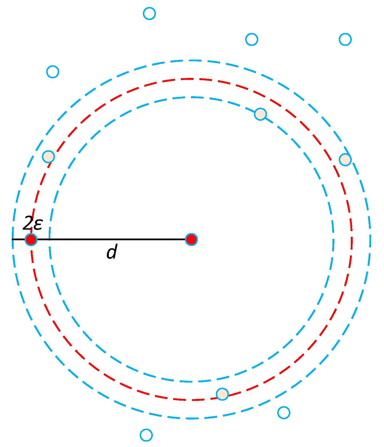
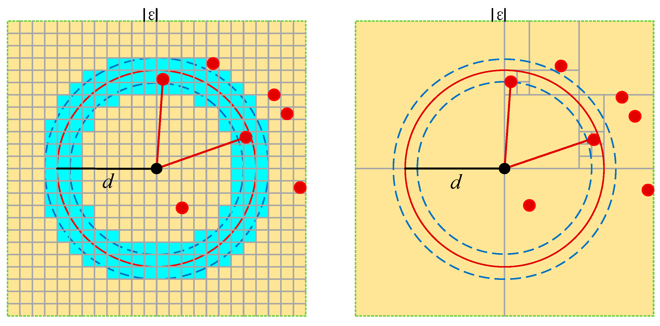
Let d denote the distance of one point-pair in a given 4-points base in the reference point cloud P, the 4PCS requires extracting all point-pairs with the same distance, which could be equivalent to a classical incidence problem between spheres and points in 3D, i.e., drawing a sphere with radius d centered at each point and then getting all points intersecting with it [13]. In the practical calculation, the range of the distance is relaxed to be approximately d with a given margin , i.e., , and the graph is shown as Figure 3. Through the above analysis, candidate point-pairs extraction could be achieved by efficient computation of incidences between spheres and point cloud, which could be finished by use of a rasterization approach [14]. Put the target point cloud into a 3D grid with cell size , in which the sphere with radius d is rasterized. All points falling in those cells (as well as their neighbors) encountered by the sphere are enumerated. Then, all candidate point-pairs could be extracted successfully, which are used to find all candidate 4-points congruent bases.
In Figure 4a, both and define a coplanar 4-points base under affine transformation, and corresponding and in Figure 4b could arbitrarily rotate around the intersection . It is obvious that and as well as and are both defined under affine transformation, but only the former is the right coplanar 4-points congruent base. Therefore, the candidate coplanar 4-points congruent base set is a super set, in which all noncoplanar 4-points congruent bases should be eliminated in order for more accurate results.
For the Super4PCS registration algorithm, the challenge is how to extract the accurate coplanar 4-points congruent base set by matching the corresponding angles between the given base in the reference point cloud P and the candidate base in target point cloud Q. This problem could be solved by use of a unit sphere rasterization approach according to the mapping relationship between angles and vector indices.
Suppose a given coplanar 4-points base is in the reference point cloud P, and let and . Let and be the corresponding affine invariant ratios. The steps of the coplanar 4-points congruent base set extraction with Super4PCS could be described as follows:
- Extract candidate point-pairs sets and from the target point cloud Q according to the distance constraint condition.
- Build a grid G with cell size .
- For vector and , traverse the candidate point-pairs set , calculate all possible intersections according to the affine invariant ratio , and, respectively, store the intersections in grid G and normalized vectors with the same orientation in the corresponding vector indices.
- For vector and , traverse the candidate point-pairs set , calculate all possible intersections according to the affine invariant ratio , and, respectively, store the intersections in grid G and normalized vectors with the same orientation in the corresponding vector indices.
- Let θ denote the angle between the two point-pairs in the given base , and extract all point-pairs according to the intersections stored in grid G and the corresponding vector indices, the angles of which are equal to θ.
3. Methodology
For 4PCS and Super4PCS algorithms, the coplanar 4-points congruent base sets are extracted under some condition constraints, including the same distance of point-pairs, the same affine invariant ratios and the same angles. In the strict sense, the coplanar 4-points congruent base is just a special congruent base, which means that both 4PCS and Super4PCS registration algorithms are only suitable for those point clouds with the same scale. Moreover, in the process of the 4-points congruent base set extraction, some local features associations of point clouds have not been considered, which may have some effect on the efficiency and precision. Therefore, a new Generalized Super 4-points Congruent Sets (G-Super4PCS) registration algorithm has been proposed in this paper. The new algorithm firstly introduces a key-scale rough estimation approach for SfM and TLS key point clouds.; Instead of the traditional 4-points congruent base, this algorithm defines a new generalized super 4-points congruent base which combines geometric relationship and local features including local roughness and normal vector of rock surface. Then scale adaptive optimization and candidate point-pairs extraction could be finished by combination of local roughness and distance constraint condition. The congruent base set could be further filtered with the local normal vector, which largely reduces times of rigid transformation verification, and improves the efficiency and precision of the registration algorithm. The flowchart of G-Super4PCS algorithm is shown as Figure 5.
3.1. Key-Scales Rough Estimation for SfM and TLS Key Point Clouds
Scale estimation is the key and precondition for registration of point clouds with different scales. The scale estimation methods could be divided into two groups [15]: the first one is to directly estimate the scale ratio of the two point clouds; and the second one is to estimate the scale for each point cloud. In this paper, a key-scale rough estimation approach based on spin images and cumulative contribution rate of PCA has been used for registration of SfM and TLS point clouds.
3.1.1. Spin Images
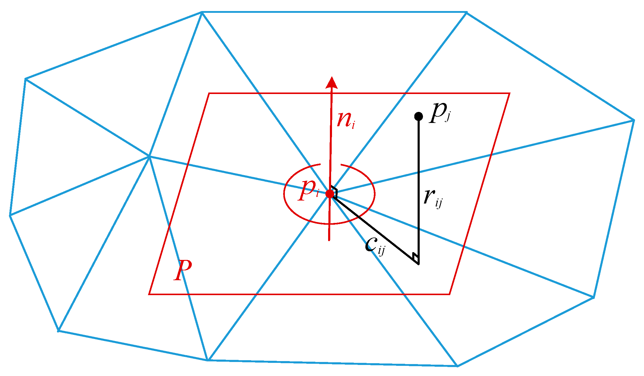
A spin image is a local feature descriptor for a 3D point, which describes local geometry by a 2D distance histogram about the 3D point and its neighbors. The generation of spin image is closely associated to point cloud normal vectors. An oriented-point is defined by a point in a point cloud P as well as its unit normal vector , which is used to be the central axis of cylindrical coordinates. For any other point near , and , respectively, denote distances along the unit normal vector and the tangent plane at , the graph of which is shown as Figure 6.
and could be calculated by Equation (4).
where , . Let w denote the spin image width, then and . Discretize distances into a grid and vote to a 2D distance histogram of bins, and then a spin image is generated.
Generally, the spin image width is related to the grid size () and its cell size. The grid size decides the spin image resolution, and the larger the grid size is, the higher the resolution is. However, the grid size should be set neither too large nor too small, which would not well describe the difference of spin images. For the experimental data in this paper, the grid size is set to . Therefore, the spin image width changes with the cell size. As the key-scales rough estimation method only needs to obtain the scale ratio between the two point clouds, the spin image width is actually represented by the cell width in this paper.
3.1.2. Relationship of Spin Image and Point Cloud Scale
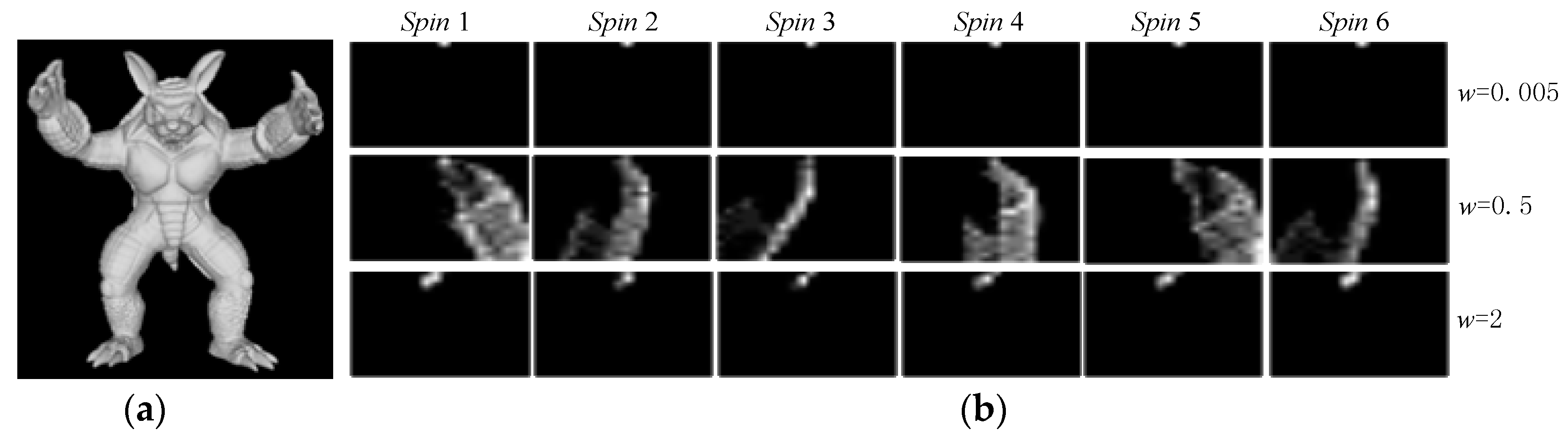
As a spin image is a feature descriptor which is not scale invariant, the image width has a large effect on local geometry description. Figure 7a shows an original point cloud, and Figure 7b shows the corresponding spin images (Spin 1, Spin 2, …, Spin 6) at different image widths.
When the image width is too small, as shown in the top row of Figure 7b, the local geometry cannot be expressed correctly with spin images, the reason of which is that for any object, its surface can be regarded as flat in an extremely small locality. In this case, all spin images look the same or very similar to each other, because they all describe a plane. Conversely, as shown in the bottom row of Figure 7b, the local geometry still cannot be described correctly with spin images when the image width is too large. In this case, all 3D points may fall in the same bin (or just in few bins) of a histogram for a spin image, which would make all spin images very similar to each other. Therefore, it can be concluded that the similarity between spin images has a minimum at a certain width. Moreover, spin images keep the most difference from each other at the minimum (as shown in the middle row of Figure 7b). That is to say, the real scale of point cloud could be estimated according to the optimal width of spin images.
3.1.3. Cumulative Contribution Rate of PCA Based on Spin Image
Principal Components Analysis (PCA) is a statistical procedure that uses an orthogonal transformation to convert a set of observations of possibly correlated variables into a set of values of linearly uncorrelated variables [16]. The similarity between spin images could be described by the cumulative contribution rate of PCA in special dimension as well as special space. The lower the cumulative contribution rate is, the more dissimilar spin images are. Let denote a spin image with bins, then it can be described with an m2-dimension vector . After performing PCA on a set of spin images , m2 eigenvectors with m2-dimension, , as well as corresponding real eigenvalues, , could be obtained. Let , then the cumulative contribution rate of the first d-dimension principal components, , could be defined as follows:
3.1.4. Key-Scale Estimation of Point Clouds
The idea of key-scale estimation is to determine the optimal spin image width when the value of cumulative contribution rate is minimum. It is difficult to show the dissimilarity between spin images if the spin image width w is too large or too small compared to the object itself.
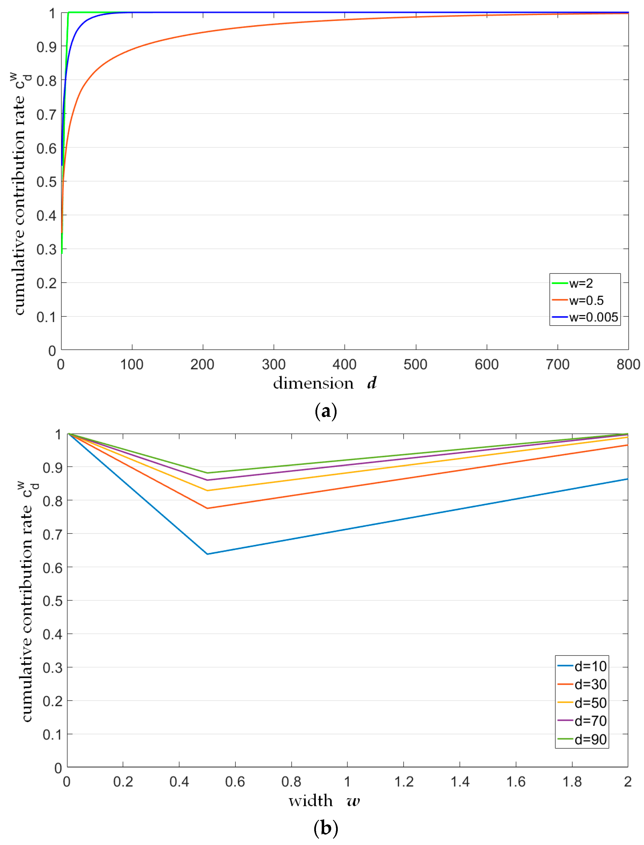
Figure 8 describes how the cumulative contribution rate changes with dimension d and spin image width w. In Figure 8a, it is obvious that the cumulative contribution rate increases monotonically with dimension d when spin image width w is fixed. Besides, the cumulative contribution rate curves quickly approach 1 when and , while the curve at increases more slowly, which means that spin images are very dissimilar with each other. In other words, when dimension d is fixed (such as d = 100), the figure visually shows that the value of the cumulative contribution rate at is lower than that at and . Figure 8b describes a group of cumulative contribution rate curves change with different spin image width w for fixed dimensions d (d = 10, 30, 50, 70 and 90), which shows the above results more clearly. In this figure, all contribution rate curves get the minimum at , where the corresponding spin images are most dissimilar. Therefore, corresponds to the key-scale of the point cloud. With the relationship between the key-scale and the spin image width, it is not difficult to conclude that the spin image width is a variable for the key-scale rough estimation, the optimal value range of which appears near the minimum of cumulative contribution rate.
With the scale rough estimation method mentioned above, the key-scales of the SfM and TLS key point clouds could be estimated; the results of which would be used for further registration process.
3.2. Definition for Generalized Super 4-Points Congruent Base Set
In order to extract generalized super 4-points congruent base set more accurately, this paper introduces local roughness of rock surface, which is defined as the distance between each point in point cloud and the plane fitted by all of its nearest points in the spherical neighborhood of radius r centered at . Suppose the radius r is changed with the scale of point cloud; then the local roughness of point is proportional to the scale. The above characteristic contributes to improving the precision of candidate point-pairs extraction.
Based on the coplanar 4-points congruent base, generalized super 4-points congruent base can be defined as follows: Let P and Q denote two point clouds with different scales under rigid transformation, and and denote corresponding surfaces. Figure 9 shows the graph of a pair of generalized super 4-points congruent base, and lines with arrow mean normal vectors of points.
Let and denote the key-scales of two point clouds estimated with the scale rough estimation method introduced in Section 3.1. For one given coplanar 4-points base in surface and another coplanar 4-points base in surface , if and are the generalized super 4-points congruent base, they have to satisfy the following fundamental conditions:
- The affine invariant ratios of and are equal to each other, i.e., and , where have been defined in Equation (2).
- The angles between the two point-pairs in and are equal to each other, i.e.,.
- The distance of corresponding point-pairs in and are proportional, i.e., and , where have been defined in Equation (3).
- The normal vector angles of corresponding points in and are equal to each other, which is shown as Equation (6).
- The local roughness and of corresponding points in and are proportional to each other in spherical neighborhoods of radius r and kr, which is shown as Equation (7).Let , then Equation (7) could be written as follows:
Figure 10 reflects the relationship of generalized super 4-points congruent base, local roughness and scales of point clouds. In the figure, denotes the given 4-points base in point cloud P, denotes the corresponding congruent base in point cloud Q, and denotes the base performed scale adjustment.
3.3. Scale Adaptive Optimization and Candidate Point-Pairs Extraction
The key-scale estimation method for point clouds determines the optimal width w by searching the minimum of cumulative contribution rate based on spin images. As the optimal width w may be valid in an extremely small range, it is difficult to get the exact value with this method. Therefore, this paper makes a further adaptive optimization process about the width w during the candidate point-pairs extraction.
Figure 11a shows a coplanar 4-points base in point cloud P, and Figure 11b shows the distance indexing sphere of the two corresponding point-pairs in point cloud Q. After rasterization for distance indexing sphere, the candidate point-pairs could be extracted. The 2D profile of the rasterized sphere is shown as Figure 12.
Suppose a refined scale ratio, where denotes a slack variable, which could be set according to the experimental data and the result of key-scales rough estimation. The scale adaptive optimization is to find the optimal in the range of . The errors of local roughness and distance are both closely related with the value of . The total error can be expressed as Equation (9).
where means the deviation of mean distance; means the deviation of normalized distance between the given point-pairs in point cloud P and the i-th candidate point-pairs in point cloud Q; and . The candidate point-pairs here are extracted at , which satisfy Condition 3 of generalized super 4-points congruent base definition. means the deviation of mean local roughness. Similarly, and mean the deviation of normalized local roughness between the given point-pairs in point cloud P and the i-th candidate point-pairs in point cloud Q, and .
The total error has the minimum at the optimal accurate scale, which can be calculated by parabola fitting. Correspondingly, the candidate point-pairs are the optimal ones for generalized super 4-points congruent base set extraction.
3.4. Extraction of Generalized Super 4-Points Congruent Base Set
In this paper, a two-step method has been proposed in order to extract generalized super 4-points congruent base set from two groups of candidate point-pairs and with high efficiency and high accuracy.
The first step filters candidate point-pairs according to the constraint condition that the angles of normal vectors between the point-pairs in the given base and the corresponding ones in the candidate point-pairs are equal to each other. Figure 13 plots a graph for the angles of normal vectors between point-pairs in given base and the corresponding ones in the candidate point-pairs sets. For a given base in point cloud P, normal vectors of each point are respectively denoted by , , and , where, denotes the angle of normal vectors and , and denotes the angle of normal vectors and . Similarly, for candidate point-pairs sets and in point cloud Q, denotes the angle of corresponding normal vectors and , and denotes the angle of corresponding normal vectors and . For point-pairs from the candidate point-pairs sets, if or , the point-pairs are preserved; otherwise, they are rejected.
In the second step, in combination of the affine invariant ratios of the given base and the two corresponding candidate point-pairs, two sets of possible intersections {} and in point cloud Q are obtained. Both intersections {} and as well as vectors of their corresponding point-pairs are, respectively, stored in a 3D grid G and vector indices. Then, with the unit sphere rasterization approach mentioned in Section 2.2, let each intersection in {} be the center of a unit sphere, and find the intersection from which fall in or on the edge of the rasterized unit sphere according to the mapping relationship between angles and vector indices. If is not empty, the point-pairs correspond to and in point cloud Q constitute a coplanar 4-points base which is congruent with the given base in point cloud P. With the above process, all generalized super 4-points congruent bases could be extracted successfully.
3.5. Algorithm Description of G-Super4PCS
Having stated the above, the procedures of G-Super4PCS could be described as follows:
- Build multi-dimension eigenvectors with spin images, and estimate key-scales of SfM and TLS key point clouds according to the relationship between the similarity of spin images and cumulative contribute rate curves of PCA.
- Extract candidate point-pairs from the target point cloud, the distances of which are proportional to the ones of the given base in the reference point cloud. Meanwhile, the accuracy of candidate point-pairs extraction has been improved greatly by the local roughness constraint as well as scale adaptive optimization.
- Extract all generalized super 4-points congruent bases from candidate point-pairs according to Constraint Conditions 1, 2 and 4 mentioned in Section 3.2, and then calculate the rigid transformation parameters.
- Select L groups of generalized super 4-points congruent bases with RANSAC to test, and find the optimal registration parameters with the LCP.
- Perform ICP algorithm on the SfM dense point cloud and TLS point cloud registered with the parameters calculated by Steps 1–4 in order to refine the registration results.
4. Experiment and Discussion
In this Section, the developed algorithm would be verified by use of the columnar basalt data acquired in Guabushan National Geopark in Jiangsu Province, China. The experiment data include digital images and TLS point cloud, which are, respectively, acquired by Fujifilm X-T10 digital camera (produced by Japan’s Fuji Photo Film) and FARO Focus3D X330 terrestrial laser scanner (produced by FARO company in Lake Mary, Florida), the resolution (point spacing on the object surface) and the ranging precision of which were, respectively, set to 0.006 m and 0.002 m. The dimensions of the measured geological research area are approximately , which is shown as Figure 14.
The experiment firstly takes the SfM key point cloud and the TLS key point cloud, respectively, extracted from digital images and the original TLS point cloud as data sources for rough registration, on the basis of which performs ICP algorithm on the SfM dense point cloud and the original TLS point cloud in order to refine the registration results. The SfM key point cloud (Figure 15a) and TLS key point cloud (Figure 15b) are shown as Figure 15. The SfM key point cloud, as the reference point cloud, has about 5194 points, and the TLS key point cloud, as the target point cloud, includes approximately 5326 points.
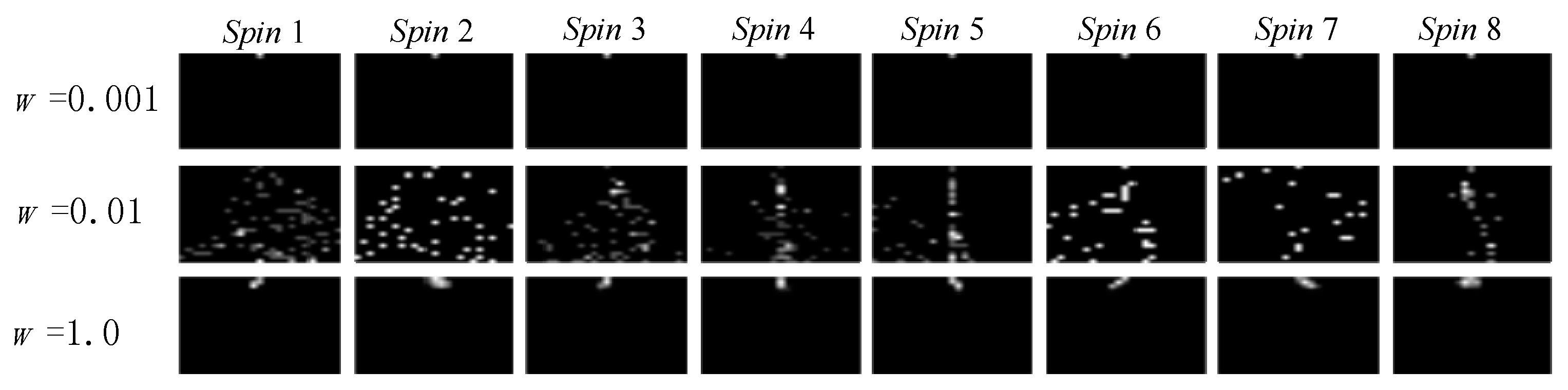
A scale rough estimation is performed on the two point clouds. The size of spin image is set to pixels. Figure 16 and Figure 17 show spin images (Spin 1, Spin 2, …, Spin 8) of some 3D points at different image width (w = 10−4, 0.005 and 0.5 for SfM key point cloud; w = 0.001, 0.01 and 1.0 for TLS key point cloud). In the figures, it can be seen that spin images of the two key point clouds change with the image width, and are rather dissimilar at w = 0.005 (for SfM key point cloud) and w = 0.01 (for TLS key point cloud), which possibly approach the real key-scales.
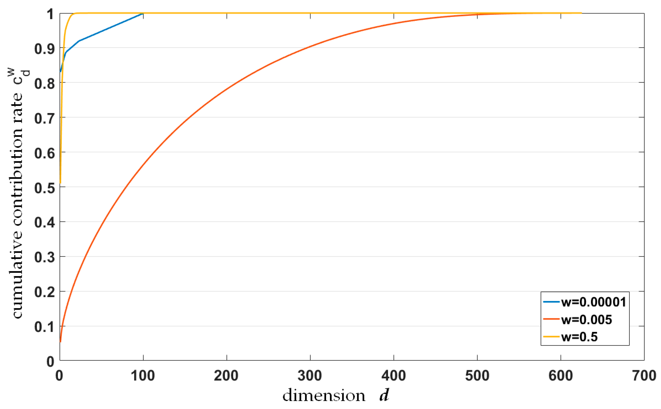
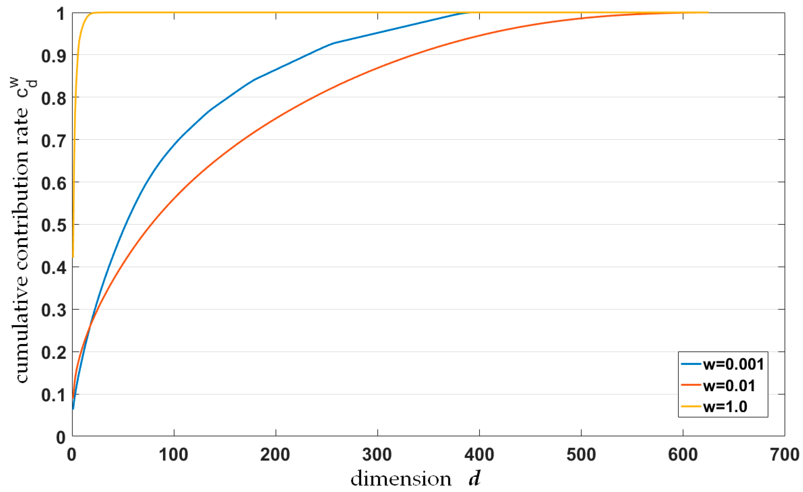
Each spin image generates a eigenvector. The cumulative contribution rate could be calculated by performing PCA on these eigenvectors, the curves of which are shown in Figure 18 (for SfM key point cloud) and Figure 19 (for TLS key point cloud). The curve charts depict the relationship between cumulative contribution rates and dimension d at different image width w. The cumulative contribute rate curves for SfM and TLS key point cloud show a slowly rising trend at w = 0.005 and w = 0.01, respectively. Moreover, for the same dimension, the cumulative contribute rate is lower than that at other image widths. That is to say, the optimal key-scales of the two point clouds correspond to w = 0.005 and w = 0.01. The key-scale ratio is approximately 1/2.
The line graphs in Figure 20 and Figure 21 depict the relationship between cumulative contribution rate and image width at different dimensions. Each broken line in the figure corresponds to a special dimension. The dimension value d is in the range of with an interval of 5. Obviously, the cumulative contribution rate has the minimum at w = 0.005 (for SfM key point cloud) and w = 0.01 (for TLS key point cloud), i.e., the key-scale ratio of SfM and TLS key point cloud is about 1/2. Therefore, the results of the scale ratio estimated with the two different groups of line charts are consistent.
The SfM and TLS key point clouds are unified in the same scale, as shown in Figure 22. The red one represents the original SfM key point cloud, and the blue one represents the TLS key point cloud after scale adjustment.
The SfM key point cloud is taken as the reference point cloud, and the TLS key point cloud is taken as the target point cloud. In this experiment, the overlap between the two key point clouds is set to 0.8, and the threshold of registration precision is set to 0.1. The whole registration process is performed iteratively. The registration results of key point clouds are shown as Table 1, where LCP responses the accuracy of registration.
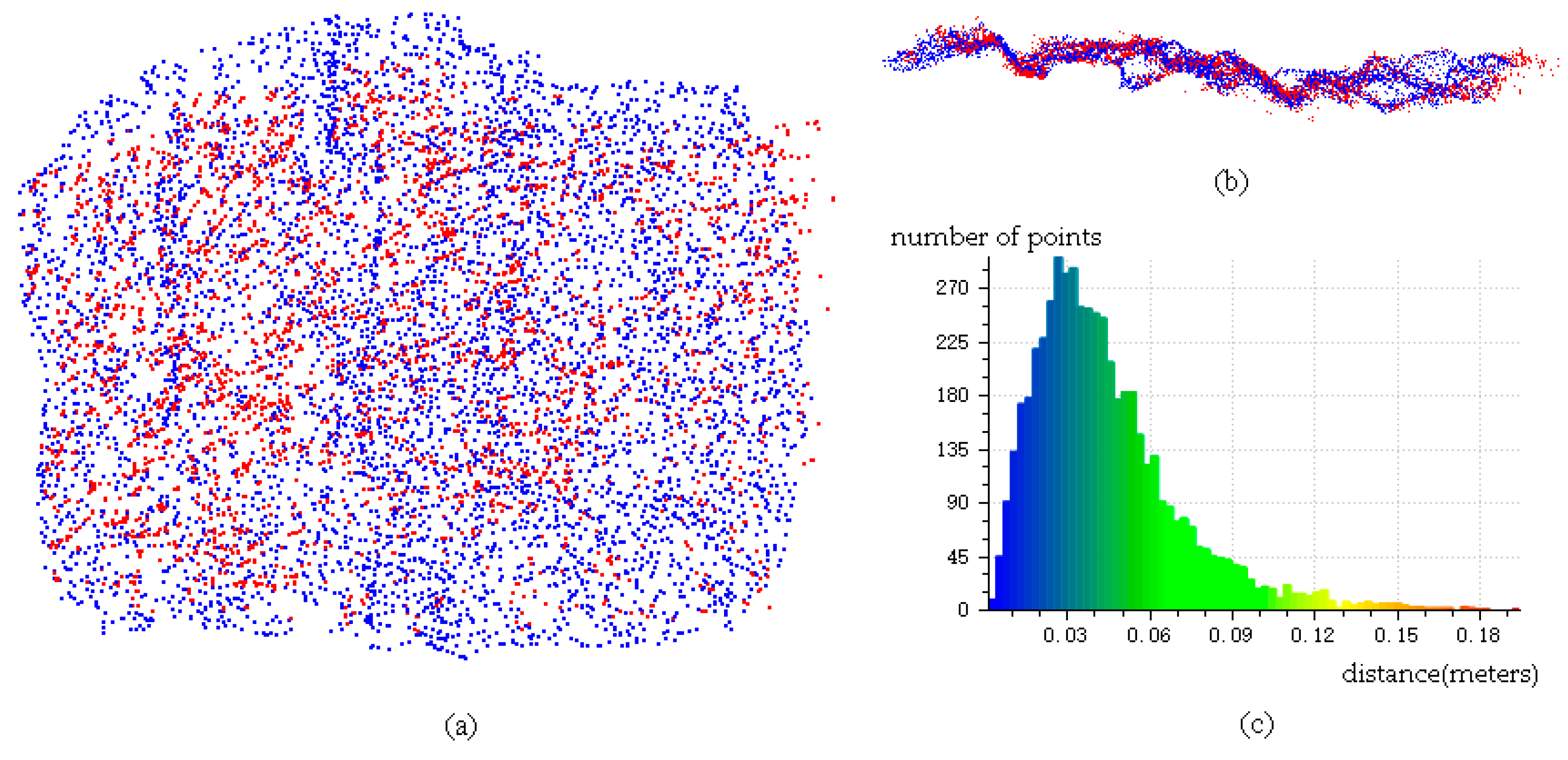
The registration results of SfM and TLS key point clouds are shown as Figure 23. Figure 23a,b, respectively, shows the front and the bottom view of the point clouds after registration. Figure 23c shows the distance distribution histogram about 5326 points in registered TLS key point cloud as well as their nearest neighbor points in SfM key point cloud. The histogram is composed of 72 bins, and the mean value and standard deviation are 0.044 m and 0.027 m, respectively.
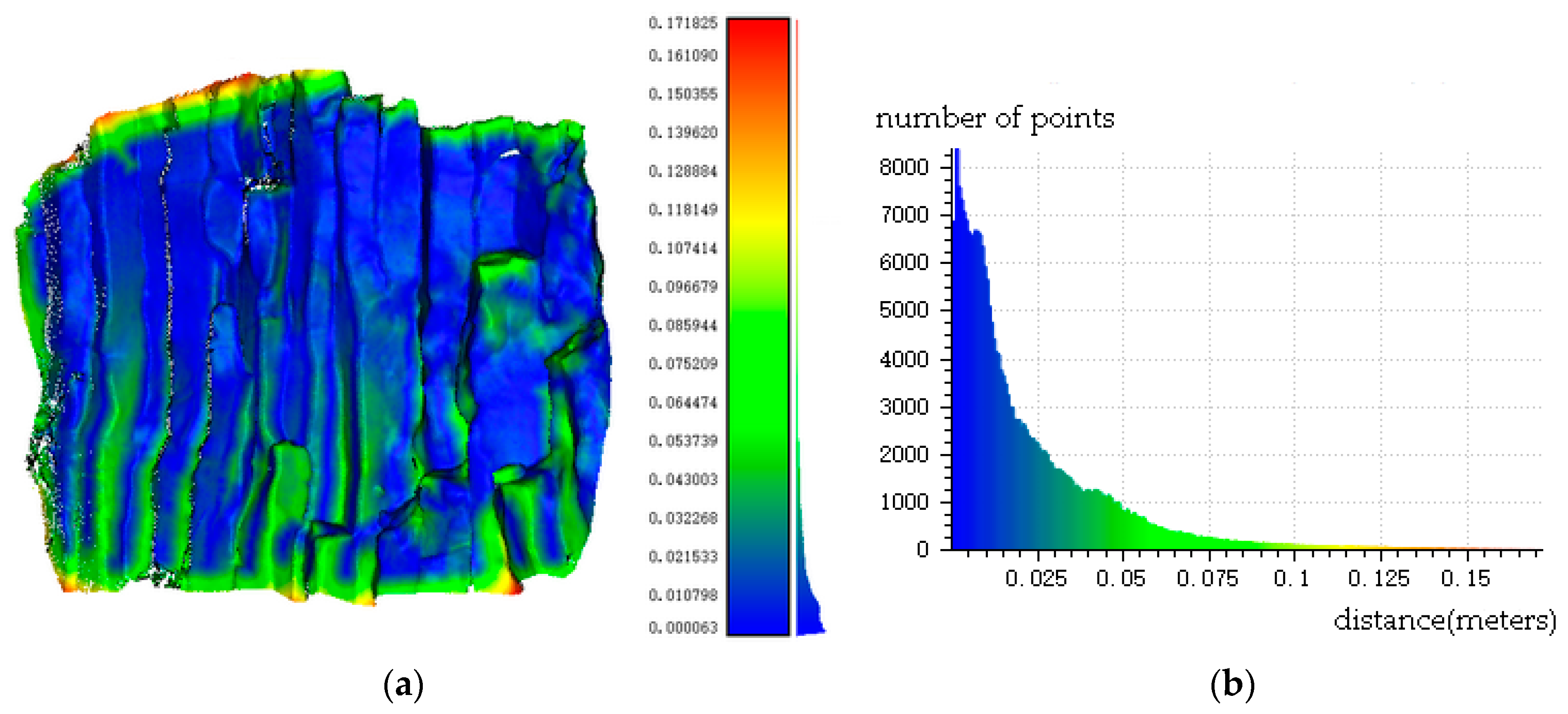
In order to improve the registration precision, taking the registration parameters of key point clouds as inputs, ICP algorithm is performed on the SfM dense point cloud and the original TLS point cloud for further registration optimization. An overlapping display for the SfM dense point cloud as well as the transformed TLS point cloud is shown as Figure 24. A hierarchical display of distances about the two registered point clouds is shown as Figure 25a, and the corresponding distance histogram is shown as Figure 25b. The mean value and standard deviation of the distance statistic results about the SfM dense point cloud and the transformed TLS point cloud are 0.022 m and 0.023 m. It can be concluded that the distances between the points and their nearest neighbor points in the overlapping part of the two point clouds are all less than 2 cm.
After fine registration with ICP algorithm, the results of registration parameters are listed in Table 2. The overlapping display of the SfM dense point cloud and the original TLS point cloud after fine registration with ICP is shown in Figure 26.
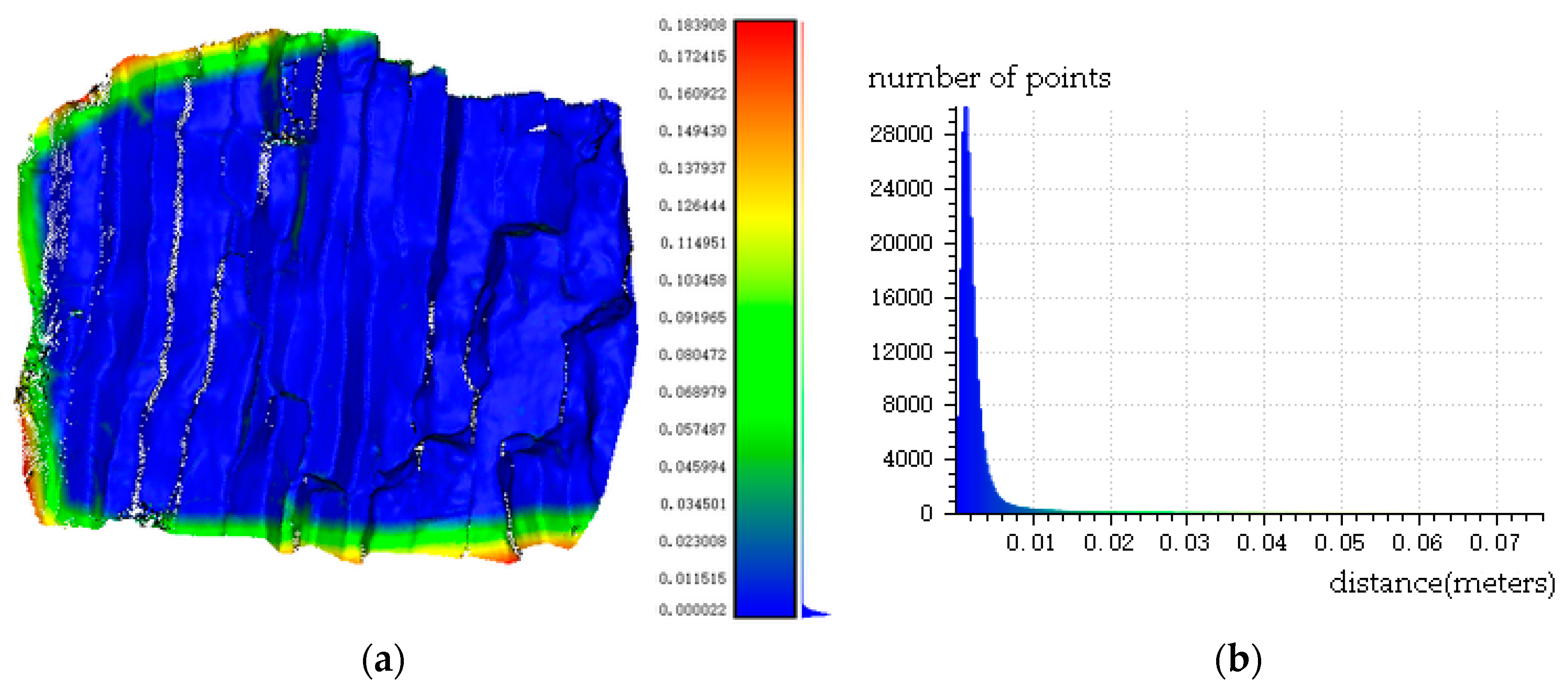
The corresponding distance hierarchical display result and the distance distribution histogram are shown as Figure 27. The mean value and standard deviation are 0.003 m and 0.005 m, respectively. According to the statistic results of the distance histogram, there are approximately 95.86% point-pairs whose distances are less than 0.01 m, which demonstrates the registration precision has been improved greatly.
With the registration result, the corresponding 3D point-pairs between the SfM dense point cloud generated from the digital images and the TLS point cloud could be obtained. Moreover, as there is a one-to-one correspondence between pixels in the digital images and 3D points in the SfM dense point cloud, the mapping relationship between the digital images and the TLS point cloud could be built, and the 2D visualization result of which is shown in Figure 28. The green rectangles represent the locations of pixels in different digital images corresponding to the same 3D point in TLS point cloud.
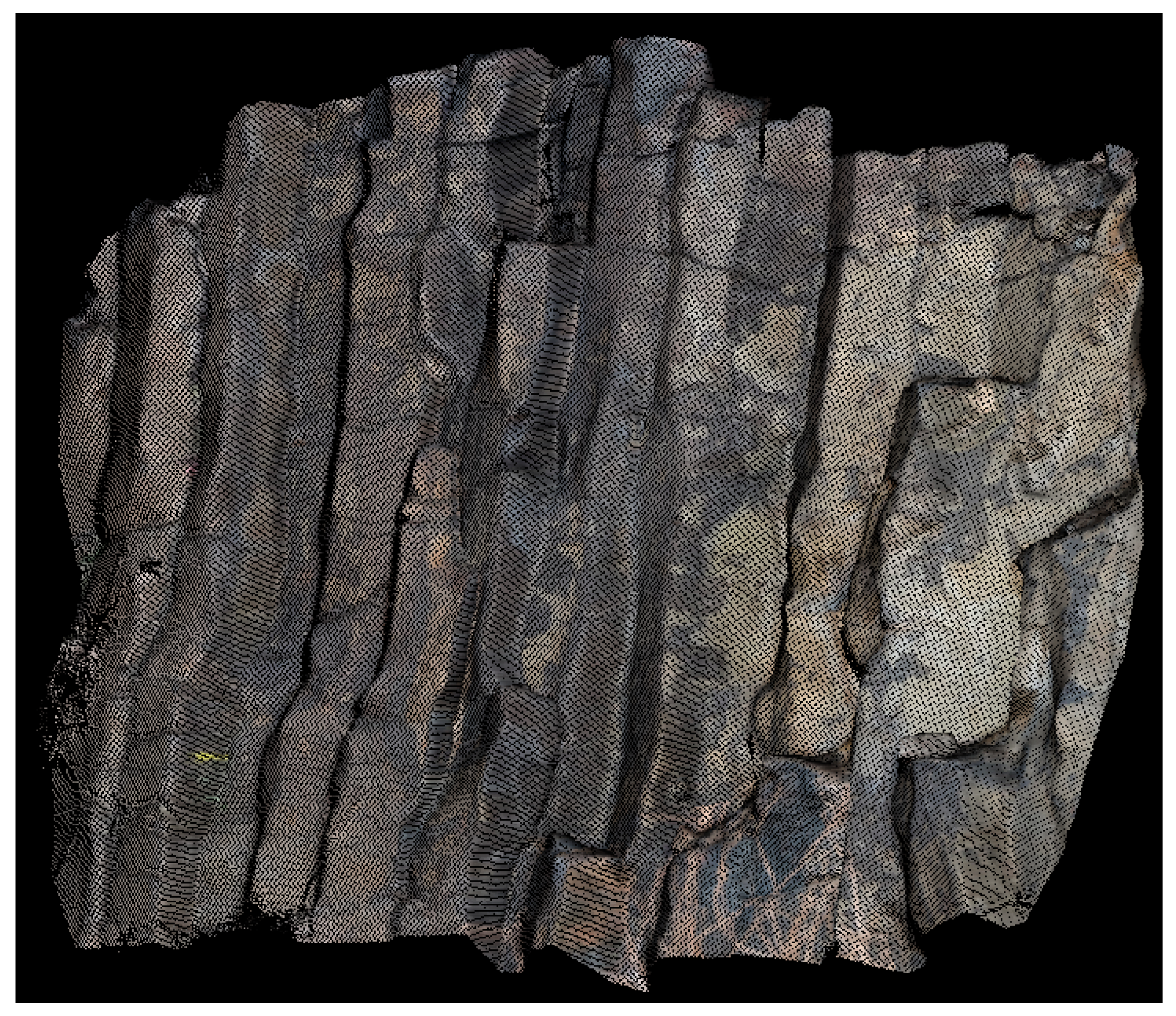
Figure 29 projects the texture information of seven digital images into the TLS point cloud according to the mapping relationship between pixels in the digital images and 3D points in the TLS point cloud. The final 3D visualization result by the fusion of spatial information of TLS point cloud and texture information of digital images is shown in Figure 30.
All of the above experimental results demonstrate that the G-Super4PCS registration algorithm could achieve fine registration between digital images and TLS point cloud without any manual interactions, and the result of which provides a crucial data basis for further integration research.
5. Conclusions
Some traditional methods usually select more than three pairs of corresponding feature points as registration primitives, and calculate the registration transformation parameters. However, such registration methods are not appropriate for some special application fields, especially for geological objects with the characteristics of complicated and irregular distribution. In recent years, 4PCS and Super4PCS algorithms have been applied more broadly, which register two point clouds that are not dependent on corresponding feature points, but on 4-points base sets satisfying the 3D affine invariant transformation. While the above algorithms are limited for those point clouds from different sensors and with various scales, this paper proposed a new registration algorithm, G-Super4PCS, for digital images and TLS point cloud in geology. This algorithm combines spin images with cumulative contribute rate for key-scale rough estimation, defines a new generalized super 4-point congruent base, and introduces the rock surface feature constraints for the scale adaptive optimization as well as high efficient extraction of the bases. The feasibility of the algorithm was validated by use of the columnar basalt data acquired in Guabushan National Geopark in Jiangsu Province, China. The results indicate that it is unnecessary for the proposed method to depend on any regular feature information of the research object itself. Moreover, although the digital images and TLS point cloud data are acquired by different sensors and with different scales, they can be registered automatically with the proposed algorithm in high efficiency and high precision. The registration results would be used for further research on rock surface extraction integrating spatial and optical information. For geological objects, the whole algorithm only involves the local orientation and roughness of point clouds, which could be calculated by point clouds normal vectors and neighbor relationship. Therefore, for point clouds data acquired by other techniques, the algorithm would be appropriate if point clouds normal vectors are provided. Besides geological objects, the registration method proposed in this paper may be valuable for some other potential application fields.
Acknowledgments
The research is supported by National Natural Science Foundation of China (No. 41471276) and Open Research Fund Program of Engineering Research Center for Rock-Soil Drilling & Excavation and Protection, Ministry of Education (No. 201508). We would like to thank all the anonymous reviewers who provided useful comments, which were incorporated into this manuscript.
Author Contributions
All the authors contributed to the development of proposed registration method and this manuscript. Rongchun Zhang and Hao Li proposed the methodology. Rongchun Zhang and Lanfa Liu performed the experiments and analyzed the results. Mingfei Wu was responsible for data acquisition. Rongchun Zhang wrote the draft of the manuscript. Hao Li guided the research and revised the manuscript.
Conflicts of Interest
The authors declare no conflict of interest.
References
- Zhang, R.; Schneider, D.; Strauß, B. Generation and Comparison of TLS and SfM Based 3D Models of Solid Shapes in Hydromechanic Research. In Proceedings of the ISPRS-International Archives of the Photogrammetry, Remote Sensing and Spatial Information Sciences, Prague, Czech Republic, 12–19 July 2016. [Google Scholar]
- Eltner, A.; Schneider, D. Analysis of different methods for 3D reconstruction of natural surfaces from Parallel-Axes UAV images. Photogramm. Rec. 2015, 30, 279–299. [Google Scholar] [CrossRef]
- Stöcker, C.; Eltner, A.; Karrasch, P. Measuring gullies by synergetic application of UAV and close range photogrammetry-A case study from Andalusia, Spain. Catena 2015, 132, 1–11. [Google Scholar] [CrossRef]
- Reiter, A.; Leonard, S.; Sinha, A.; Ishii, M.; Taylor, R.H.; Hager, G.D. Endoscopic-CT: Learning-Based Photometric Reconstruction for Endoscopic Sinus Surgery. In Proceedings of the SPIE Optics and Photonics 2016, San Diego, CA, USA, 28 August–1 September 2016. [Google Scholar]
- Opitz, R.S.; Johnson, T.D. Interpretation at the controller’s edge: Designing graphical user interfaces for the digital publication of the excavations at Gabii (Italy). Open Archaeol. 2016, 2, 1–17. [Google Scholar] [CrossRef]
- Muñumer, E.; Lerma, J.L. Fusion of 3D Data from Different Image-Based and Range-Based Sources for Efficient Heritage Recording. In Proceedings of the Digital Heritage 2015, Granada, Spain, 28 September–2 October 2015. [Google Scholar]
- Armistead, C.C. Applications of ‘Structure from Motion’ Photogrammetry to River Channel Change Studies. Doctor’s Thesis, Boston College, College of Arts and Sciences, Boston, MA, USA, 2013. [Google Scholar]
- Snavely, N.; Seitz, S.M.; Szeliski, R. Modeling the world from internet photo collections. Int. J. Comput. Vis. 2008, 80, 189–210. [Google Scholar] [CrossRef]
- Westoby, M.J.; Brasington, J.; Glasser, N.F.; Hambrey, M.J.; Reynolds, J.M. ‘Structure from Motion’ photogrammetry: A low-cost, effective tool for geoscience applications. Geomorphology 2012, 179, 300–314. [Google Scholar] [CrossRef]
- Aiger, D.; Mitra, N.J.; Cohen-Or, D. 4-points congruent sets for robust pairwise surface registration. ACM Trans. Graph. 2008, 27, 85. [Google Scholar] [CrossRef]
- Fischler, M.A.; Bolles, R.C. Random sample consensus: A paradigm for model fitting with applications to image analysis and automated cartography. Commun. ACM 1981, 24, 381–395. [Google Scholar] [CrossRef]
- Mellado, N.; Aiger, D.; Mitra, N.J. Super 4pcs fast global pointcloud registration via smart indexing. Comput. Graph. Forum 2014, 33, 205–215. [Google Scholar] [CrossRef]
- Pach, J.; Sharir, M. Geometric incidences. Contemp. Math. 2004, 342, 185–224. [Google Scholar]
- Gavrilov, M.; Indyk, P.; Motwani, R.; Venkatasubramanian, S. Combinatorial and experimental methods for approximate point pattern matching. Algorithmica 2004, 38, 59–90. [Google Scholar] [CrossRef]
- Lin, B.; Tamaki, T.; Zhao, F.; Raytchev, B.; Kaneda, K.; Ichii, K. Scale alignment of 3D point clouds with different scales. Mach. Vis. Appl. 2014, 25, 1989–2002. [Google Scholar] [CrossRef]
- Hotelling, H. Analysis of a complex of statistical variables into principal components. J. Educ. Psychol. 1933, 24, 417. [Google Scholar] [CrossRef]
Figure 1.
The flowchart of the 4-Points Congruent Sets (4PCS) algorithm.
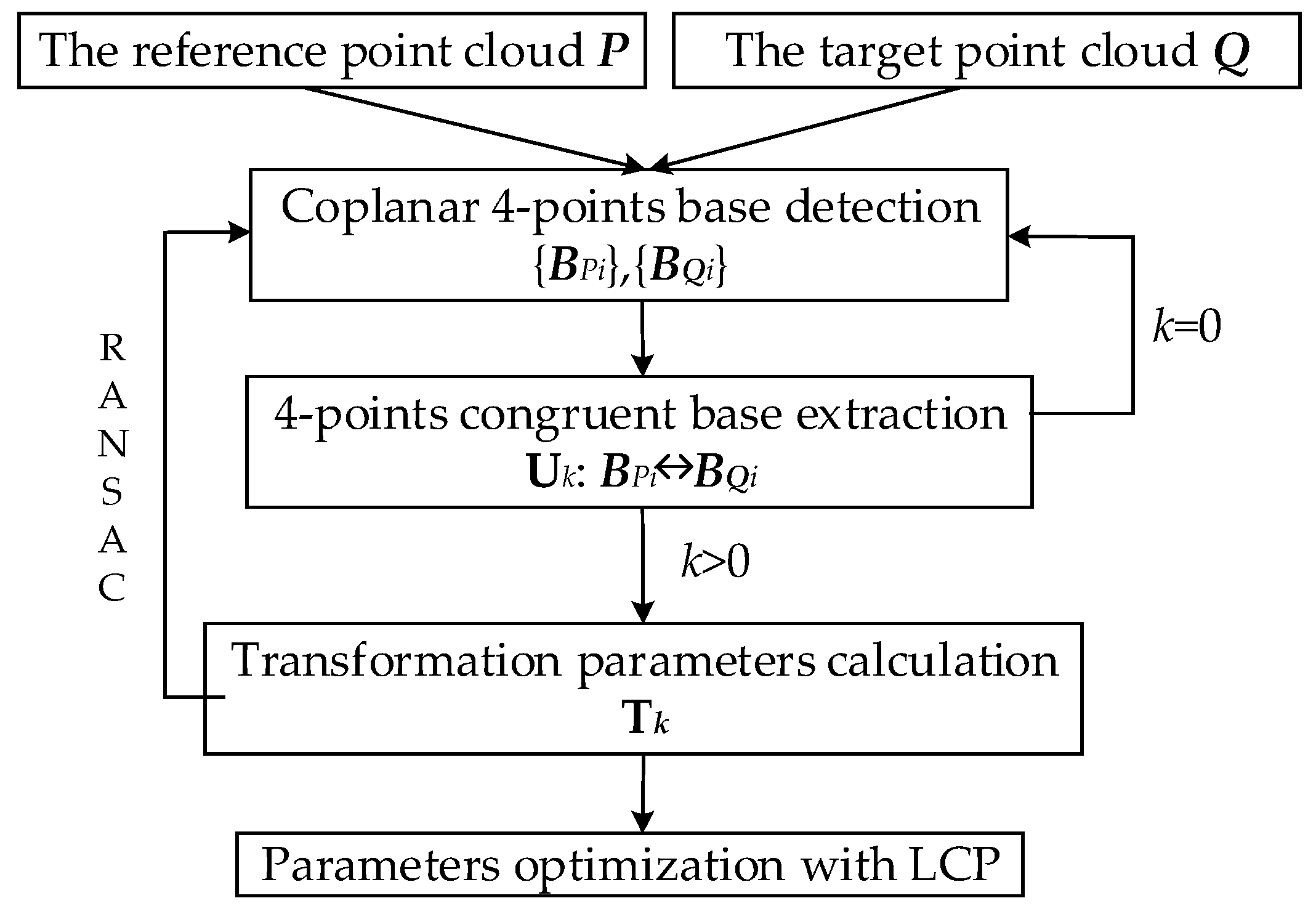
Figure 2.
A coplanar 4-points congruent base: (a) one coplanar base in surface ; and (b) the congruent coplanar base in surface .
Figure 2.
A coplanar 4-points congruent base: (a) one coplanar base in surface ; and (b) the congruent coplanar base in surface .
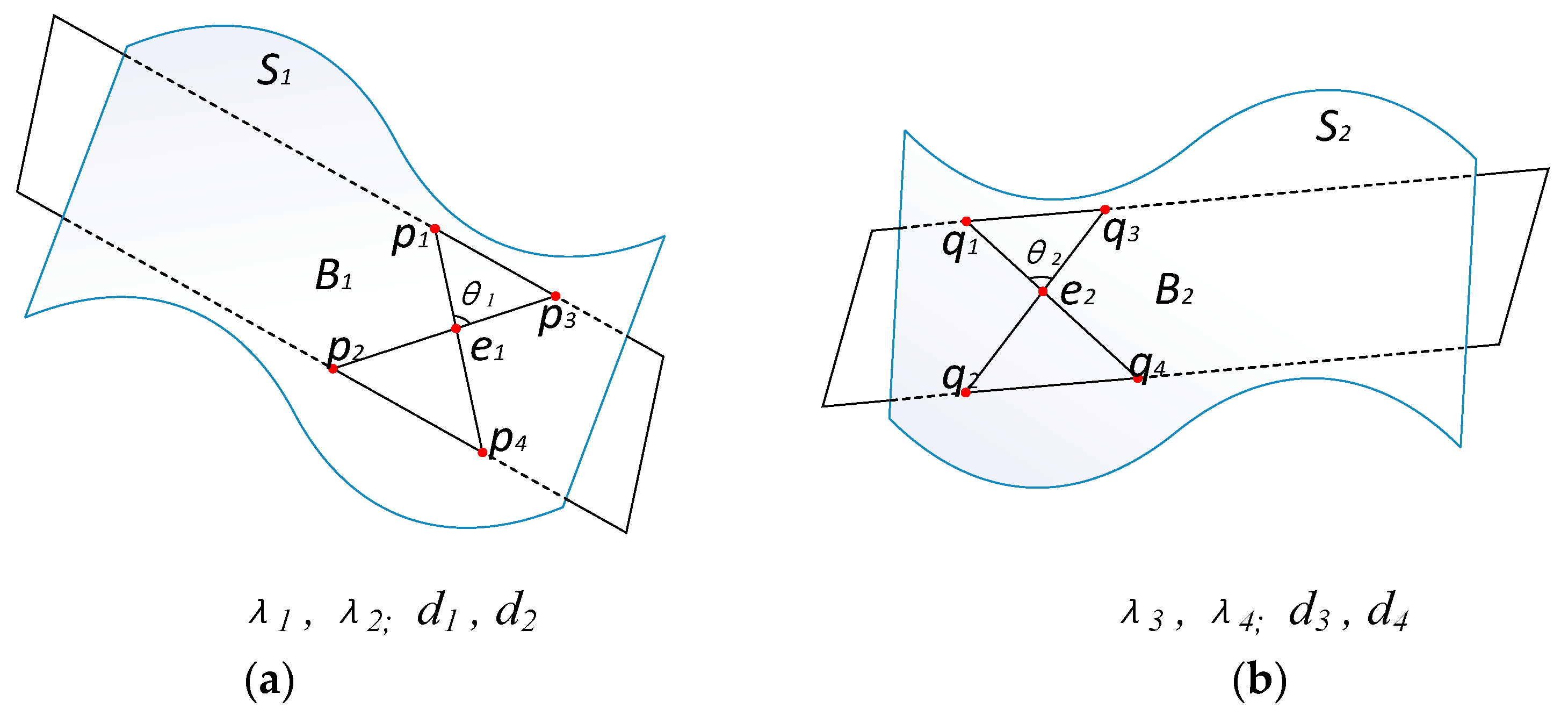
Figure 3.
The graph of incidences between the sphere and 3D points.

Figure 4.
Non-uniqueness of coplanar 4-points base under affine transformation: (a) a given coplanar 4-points base in reference point cloud P; and (b) the possible corresponding coplanar 4-points bases in target point cloud Q.
Figure 4.
Non-uniqueness of coplanar 4-points base under affine transformation: (a) a given coplanar 4-points base in reference point cloud P; and (b) the possible corresponding coplanar 4-points bases in target point cloud Q.

Figure 5.
The flowchart of Generalized Super 4-points Congruent Sets (G-Super4PCS) algorithm.

Figure 6.
The graph of and .

Figure 7.
(a) A point cloud of a monster; and (b) the corresponding spin images (Spin 1, Spin 2, …, Spin 6) for some points at different image widths (w = 0.005, 0.5 and 2).
Figure 7.
(a) A point cloud of a monster; and (b) the corresponding spin images (Spin 1, Spin 2, …, Spin 6) for some points at different image widths (w = 0.005, 0.5 and 2).

Figure 8.
Two examples of cumulative contribution rate curves: (a) different dimensions d for fixed spin image widths w; and (b) different spin image widths w for fixed dimensions d.
Figure 8.
Two examples of cumulative contribution rate curves: (a) different dimensions d for fixed spin image widths w; and (b) different spin image widths w for fixed dimensions d.

Figure 9.
The generalized super 4-points congruent base.

Figure 10.
The label (I) refers to the given base in point cloud P as well as its original congruent base in point cloud Q; the label (II) refers to the given base in point cloud P as well as the base in point cloud Q; and the label (III) refers to the base before scale adjustment as well as the base after scale adjustment for point cloud Q.
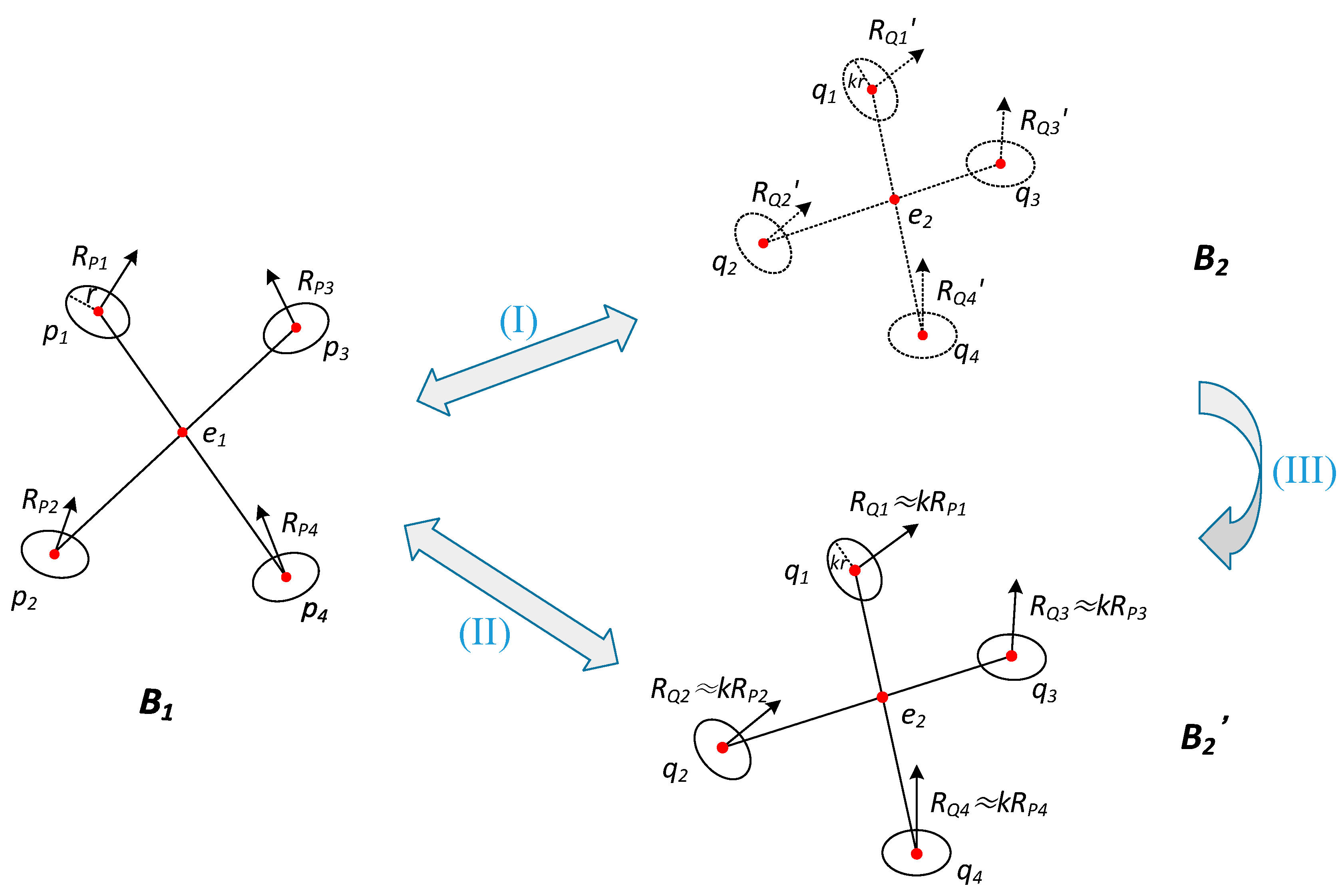
Figure 11.
(a) A coplanar 4-points base in point cloud P; and (b) the distance indexing sphere of the two corresponding point-pairs in point cloud Q.
Figure 11.
(a) A coplanar 4-points base in point cloud P; and (b) the distance indexing sphere of the two corresponding point-pairs in point cloud Q.

Figure 12.
The 2D profile of the rasterized indexing sphere.

Figure 13.
The graph for the angles of normal vectors between point-pairs in given base and the corresponding ones in candidate point-pairs sets.
Figure 13.
The graph for the angles of normal vectors between point-pairs in given base and the corresponding ones in candidate point-pairs sets.

Figure 14.
The image of the geological research area.
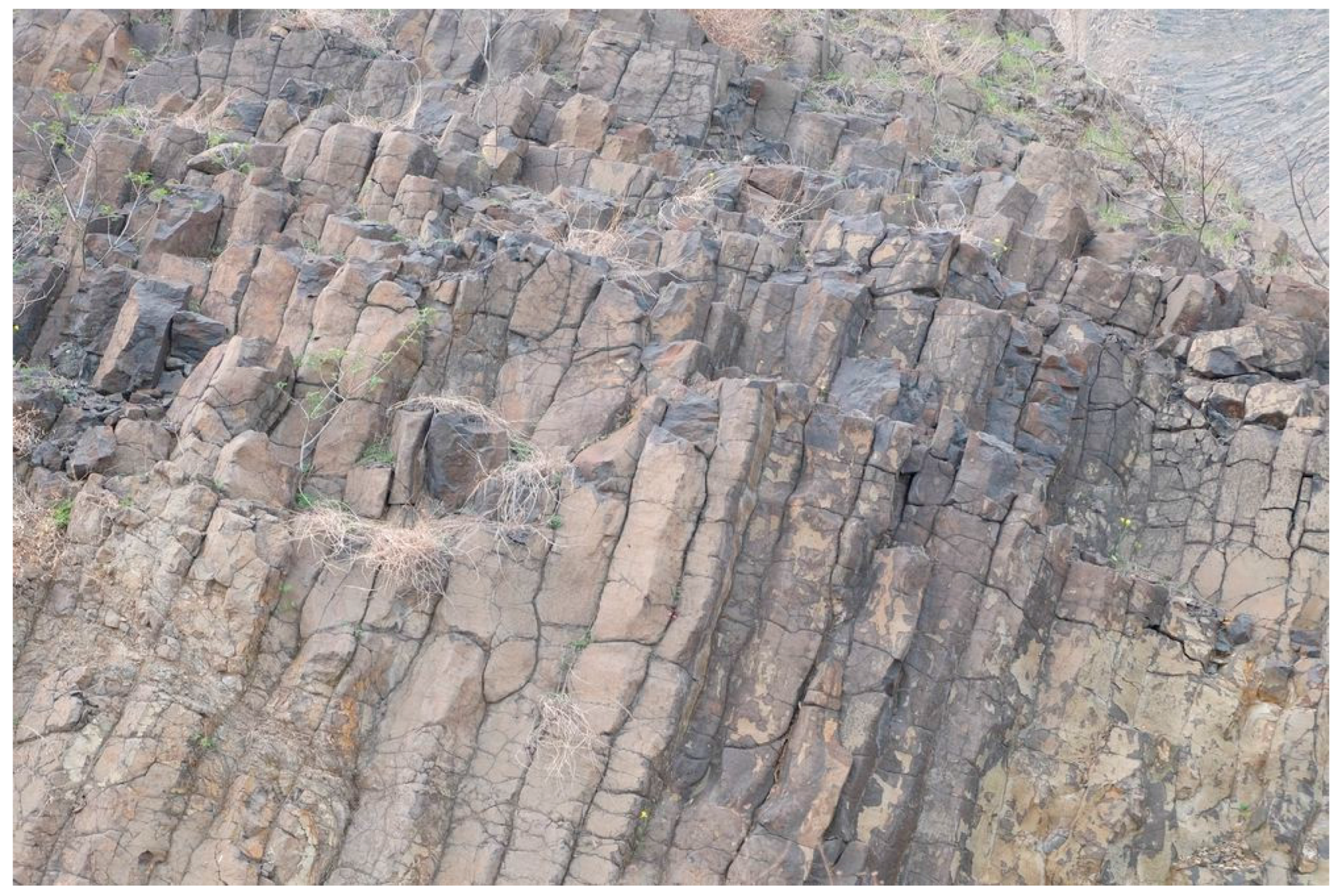
Figure 15.
(a) The SfM key point cloud; and (b) the TLS key point cloud.

Figure 16.
Spin images (Spin 1, Spin 2, …, Spin 8) of some SfM 3D points at different image width (w = 10−4, 0.005 and 0.5).
Figure 16.
Spin images (Spin 1, Spin 2, …, Spin 8) of some SfM 3D points at different image width (w = 10−4, 0.005 and 0.5).
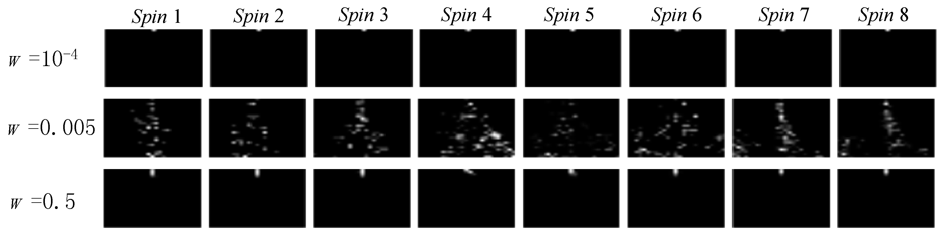
Figure 17.
Spin images (Spin 1, Spin 2, …, Spin 8) of some TLS 3D points at different image width (w = 0.001, 0.01 and 1.0).
Figure 17.
Spin images (Spin 1, Spin 2, …, Spin 8) of some TLS 3D points at different image width (w = 0.001, 0.01 and 1.0).

Figure 18.
The relationship between cumulative contribution rates and dimension d at w = 0.00001, 0.005 and 0.5 (the SfM key point cloud).
Figure 18.
The relationship between cumulative contribution rates and dimension d at w = 0.00001, 0.005 and 0.5 (the SfM key point cloud).

Figure 19.
The relationship between cumulative contribution rates and dimension d at w = 0.001, 0.01 and 1.0 (the TLS key point cloud).
Figure 19.
The relationship between cumulative contribution rates and dimension d at w = 0.001, 0.01 and 1.0 (the TLS key point cloud).

Figure 20.
The relationship between cumulative contribution rate and image width at different dimensions (SfM key point cloud).
Figure 20.
The relationship between cumulative contribution rate and image width at different dimensions (SfM key point cloud).

Figure 21.
The relationship between cumulative contribution rate and image width at different dimensions (TLS key point cloud).
Figure 21.
The relationship between cumulative contribution rate and image width at different dimensions (TLS key point cloud).
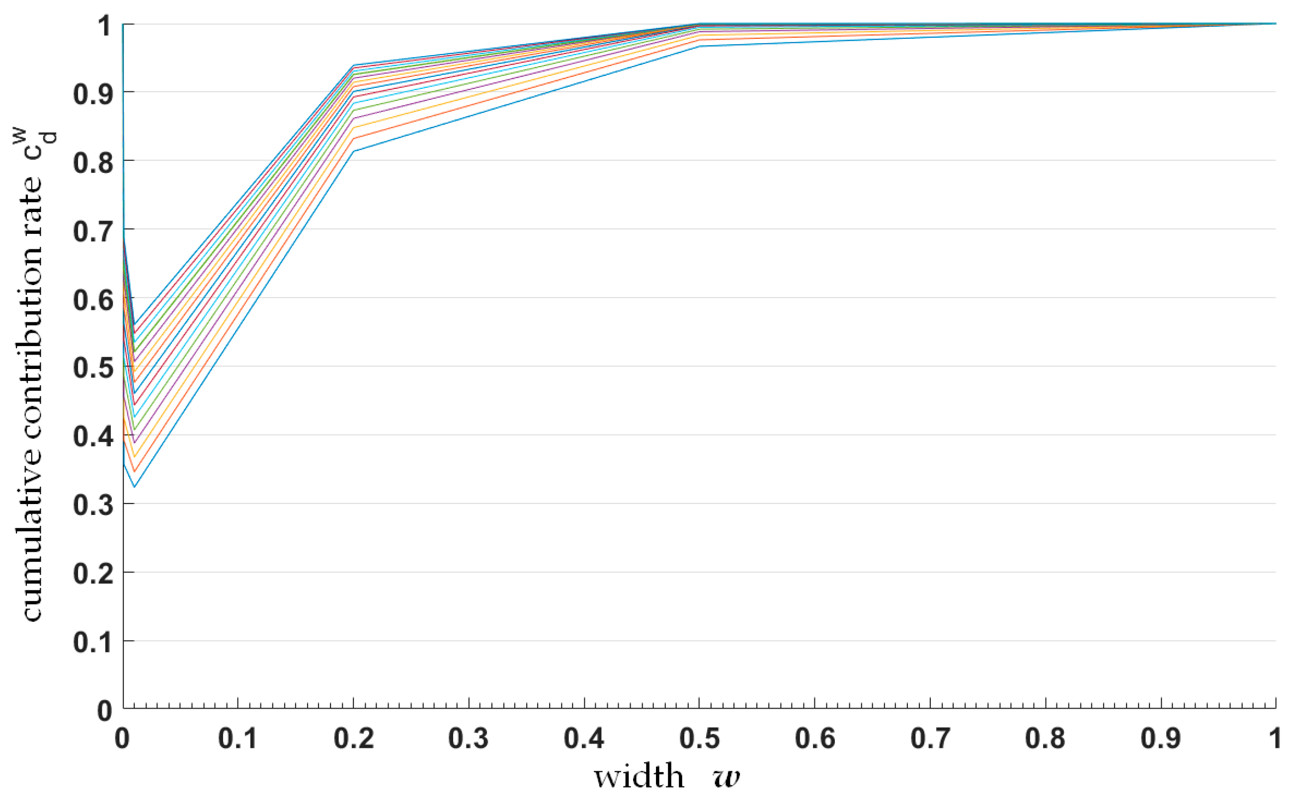
Figure 22.
SfM (a) and TLS (b) key point cloud with the same scale.

Figure 23.
(a) The front view of the two registered point clouds; (b) the bottom view of the two registered point clouds; and (c) the distance distribution histogram of the registered two point clouds.
Figure 23.
(a) The front view of the two registered point clouds; (b) the bottom view of the two registered point clouds; and (c) the distance distribution histogram of the registered two point clouds.

Figure 24.
The initial registration result of SfM dense point cloud and original TLS point cloud.

Figure 25.
(a) A hierarchical display of distances about the two registered point clouds; and (b) the corresponding distance distribution histogram.
Figure 25.
(a) A hierarchical display of distances about the two registered point clouds; and (b) the corresponding distance distribution histogram.

Figure 26.
The fine registration result with ICP.

Figure 27.
(a) A hierarchical display of distances about the two fine registered point clouds with ICP; and (b) the corresponding distance distribution histogram.
Figure 27.
(a) A hierarchical display of distances about the two fine registered point clouds with ICP; and (b) the corresponding distance distribution histogram.

Figure 28.
Pixel locations in the four images (a–d) corresponding to the same 3D point in TLS point cloud.
Figure 28.
Pixel locations in the four images (a–d) corresponding to the same 3D point in TLS point cloud.

Figure 29.
The regions with texture in (a–g) respectively shows the 3D visualization of the correspondences between different images and TLS point cloud.
Figure 29.
The regions with texture in (a–g) respectively shows the 3D visualization of the correspondences between different images and TLS point cloud.
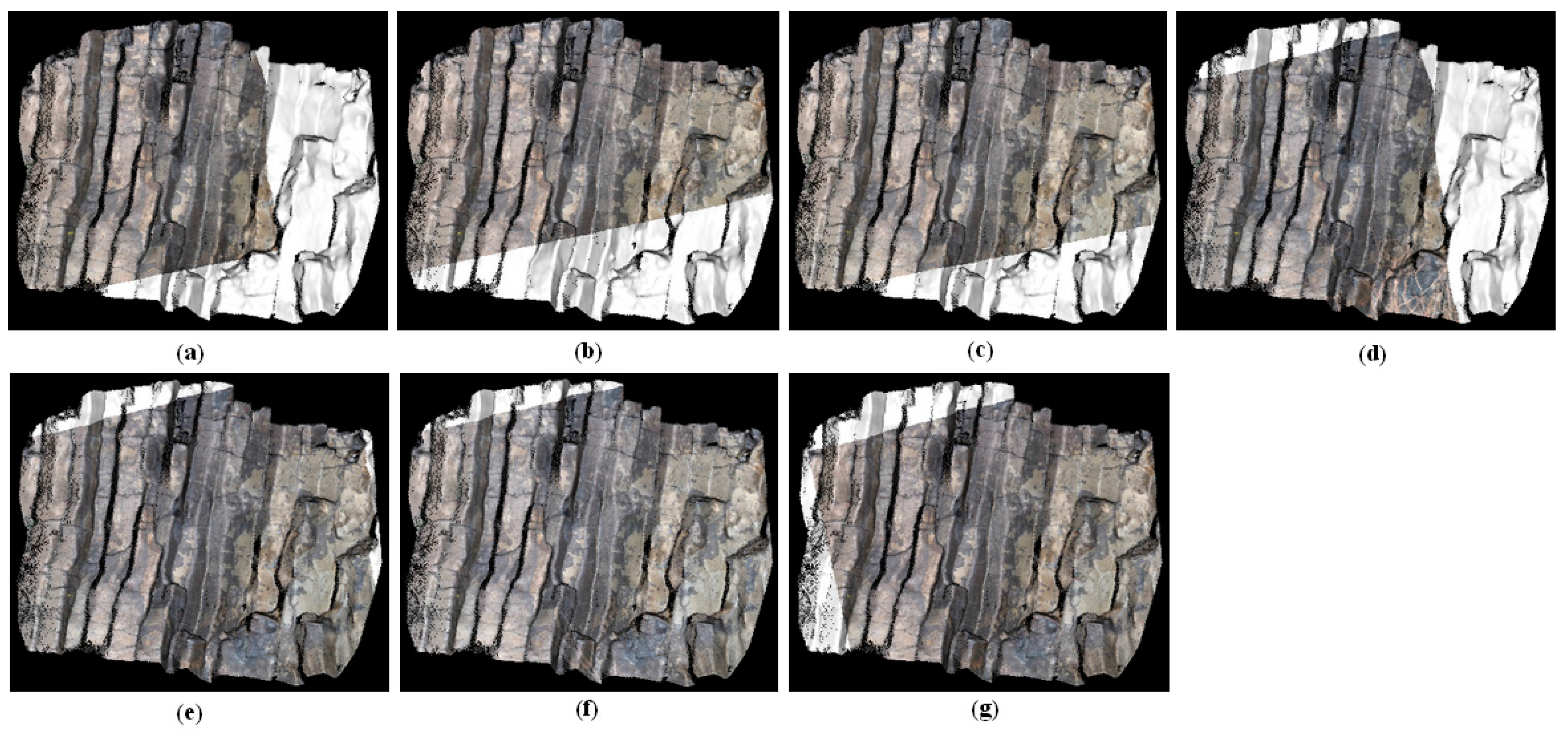
Figure 30.
3D visualization for the fusion of spatial information of TLS point cloud and texture information of digital images.
Figure 30.
3D visualization for the fusion of spatial information of TLS point cloud and texture information of digital images.

Table 1.
The results of registration parameters before ICP optimization.
| Rotation Matrix (R) | Translation (T) | Scale Ratio | LCP | ||||
|---|---|---|---|---|---|---|---|
| Before Optimization | After Optimization | The First Iteration | The Optimal Iteration | ||||
| 0.930 | 0.361 | −0.063 | −44.712 | 0.50 | 0.65 | 13.77% | 93.48% |
| 0.103 | −0.093 | 0.990 | −54.862 | ||||
| 0.352 | −0.928 | −0.124 | −46.877 | ||||
Table 2.
The results of registration parameters after ICP optimization.
| Rotation Matrix (R) | Translation (T) | RMS (meters) | ||
|---|---|---|---|---|
| 0.992 | 0.065 | −0.018 | −0.125 | 0.005 |
| −0.064 | 0.991 | 0.047 | 0.410 | |
| 0.021 | −0.046 | 0.993 | −0.081 | |
© 2017 by the authors. Licensee MDPI, Basel, Switzerland. This article is an open access article distributed under the terms and conditions of the Creative Commons Attribution (CC BY) license (http://creativecommons.org/licenses/by/4.0/).
Share and Cite
MDPI and ACS Style
Zhang, R.; Li, H.; Liu, L.; Wu, M. A G-Super4PCS Registration Method for Photogrammetric and TLS Data in Geology. ISPRS Int. J. Geo-Inf. 2017, 6, 129. https://0-doi-org.brum.beds.ac.uk/10.3390/ijgi6050129
AMA Style
Zhang R, Li H, Liu L, Wu M. A G-Super4PCS Registration Method for Photogrammetric and TLS Data in Geology. ISPRS International Journal of Geo-Information. 2017; 6(5):129. https://0-doi-org.brum.beds.ac.uk/10.3390/ijgi6050129
Chicago/Turabian StyleZhang, Rongchun, Hao Li, Lanfa Liu, and Mingfei Wu. 2017. "A G-Super4PCS Registration Method for Photogrammetric and TLS Data in Geology" ISPRS International Journal of Geo-Information 6, no. 5: 129. https://0-doi-org.brum.beds.ac.uk/10.3390/ijgi6050129
Note that from the first issue of 2016, this journal uses article numbers instead of page numbers. See further details here.