
Statistical Evaluation of No-Reference Image Quality Assessment Metrics for Remote Sensing Images

1
International School of Software, Wuhan University, Wuhan 430079, China
2
State Key Laboratory of Resources and Environmental Information System, Institute of Geographic Sciences and Natural Resources Research, Chinese Academy of Sciences, Beijing 100101, China
*
Author to whom correspondence should be addressed.
ISPRS Int. J. Geo-Inf. 2017, 6(5), 133; https://0-doi-org.brum.beds.ac.uk/10.3390/ijgi6050133
Submission received: 19 January 2017
/
Revised: 17 April 2017
/
Accepted: 25 April 2017
/
Published: 28 April 2017
Abstract
:Image quality assessment plays an important role in image processing applications. In many image applications, e.g., image denoising, deblurring, and fusion, a reference image is rarely available for comparison with the enhanced image. Thus, the quality of enhanced images must be evaluated blindly without references. In recent years, many no-reference image quality metrics (IQMs) have been proposed for assessing digital image quality. In this paper, we first review 21 commonly employed no-reference IQMs. Second, we apply these measures to Quickbird images with three different types of general content (urban, rural, and harbor) subjected to three types of degradation (average filtering, Gaussian white noise, and linear motion degradation), each with 40 degradation levels. We evaluate the robustness of the IQMs based on the criteria of prediction accuracy, prediction monotonicity, and prediction consistency. Then, we perform factor analysis on those IQMs deemed robust, and cluster them into several components. We then select the IQM with the highest loading coefficient as the representative IQM for that component. Experimental results suggest that different measures perform differently for images with different contents and subjected to different types of degradation. Generally, the degradation method has a stronger effect than the image content on the evaluation results of an IQM. The same IQM can provide opposite dependences on the level of degradation for different degradation types, and an IQM that performed well with one type of degradation may not perform well with another type. The training-based measures are not appropriate for remote sensing images because the results are highly dependent on the samples employed for training. Only seven of the 21 IQMs were found to fulfill the requirements of robustness. Edge intensity (EI) and just noticeable distortion (JND) are suggested for evaluating the quality of images subjected to average filter degradation. EI, blind image quality assessment through anisotropy (BIQAA), and mean metric (MM) are suggested for evaluating the quality of images subjected to Gaussian white noise degradation. Laplacian derivative (LD), JND, and standard deviation (SD) are suggested for evaluating the quality of images subjected to linear motion. Finally, EI is suggested for evaluating the quality of an image subjected to an unknown type of degradation.
1. Introduction
The quality of digital images can be degraded during acquisition, transmission, storage, and reconstruction by various sources of degradation, such as distortion of the spatial resolution, motion blur, and transmission noise [1]. Identifying the distortion and quantifying its impact on image quality is essential for various applications such as for monitoring image quality in quality control systems and for optimizing the output of image processing algorithms [2]. The development of effective image quality assessment is therefore necessary for these purposes [3,4].
Because human beings are generally the end user in most image processing applications, the most reliable means of assessing image quality is by subjective evaluation. A subjective image quality metric (IQM) can be computed by preparing test images, selecting an appropriate number of human observers, and obtaining their opinion based on specified criteria and conditions. Widely used subjective IQMs are mean opinion score (MOS) and difference MOS (DMOS) [5]. However, subjective IQMs require the services of multiple human observers, and are thus expensive, time-consuming, and impractical for real-time implementation. Moreover, the subjective test results depend on a number of factors that are difficult to quantify, such as the background and motivation of observers [6,7]. As a result, the development of objective IQMs is presently receiving increasing attention. The goal is to design objective IQMs that quantify the image quality automatically and yield reliable results that are well correlated with subjective assessments [8]. In general, objective IQMs can be classified into three categories according to the extent to which a reference image is required: full-reference (FR), reduced-reference (RR), and no-reference (NR). In an objective FR IQM, a reference image is required to assess the quality of the test image by comparing the extent of similarity or difference between the test image and the reference image. Objective FR IQM include the classical mean squared error (MSE), peak signal to noise ratio (PSNR), and the recently introduced structural similarity (SSIM) [9]. In an objective RR IQM, some extracted features of a reference image are required to assess the quality of a test image. Objective RR IQM include a number of IQMs such as reference reduced image quality assessment (RRIQA) [10] and C4 [11]. In an objective NR IQM, the statistical metric is calculated from the distorted image itself. Objective NR IQM include a number of IQMs such as entropy, gradient, and standard deviation [12]. In contrast to FR or RR IQM, an NR IQM to some extent calculates the quality of the test image directly according to particular criteria, rather than assessing its fidelity or similarity to the reference image. Moreover, in many image applications, e.g., image denoising, deblurring, and fusion, a reference image is rarely available for comparison with the enhanced image. Thus, the image quality must be evaluated in the absence of a reference image [13,14,15,16].
Although a number of new objective IQMs have been developed in the past few decades, the majority of these require the original undistorted image as a reference [17]. The development of objective NR IQMs is a relatively new topic in the field of image processing, and, in more recent years, a large number of NR metrics have been proposed for evaluating image quality. However, most NR metrics have been designed for gray or color images, and whether they are suitable for multi-spectral remote sensing images is still unknown. In this paper, we first review 21 commonly employed objective NR metrics. Then, we apply these measures to Quickbird images with three different contents (urban, rural, and harbor) using three types of degradation (average filtering, Gaussian white noise, and linear motion degradation), each with 40 degradation levels. We then investigate the robustness of the individual IQMs based on the criteria of prediction accuracy, prediction monotonicity, and prediction consistency. Finally, we analyze those NR metrics deemed robust, and determine representative NR metrics suitable for evaluating remote sensing images with different types of degradation.
2. Commonly Employed No-Reference Image Quality Metrics: An Overview
This section presents an overview of commonly employed objective NR IQMs proposed in recent years. These include several categories, i.e., distortion specific metrics, training-based metrics, and metrics based on natural scene statistics.
- Auto correlation (AC): Derived from the auto-correlation function. The AC metric uses the difference between auto-correlation values at two different distances along the horizontal and vertical directions, respectively. If an image is blurred or the edges are smoothed, the correlation between neighboring pixels becomes high.
- Average gradient (AG): Reflects the contrast and the clarity of the image. It can be used to measure the spatial resolution of a test image, where a larger AG indicates better spatial resolution [18].
- Blind image quality index (BIQI): A two-step framework based on natural scene statistics. Once trained, the framework requires no knowledge of the distortion process, and the framework is modular, in that it can be extended to any number of distortions [19].
- Blind image quality assessment through anisotropy (BIQAA): Measures the averaged anisotropy of an image by means of a pixel-wise directional entropy. A pixel-wise directional entropy is obtained by measuring the variance of the expected Rényi entropy and the normalized pseudo-Wigner distribution of the image for a set of predefined directions. BIQAA is capable of distinguishing the presence of noise in images [20].
- Blind image integrity notator using discrete cosine transform (DCT) statistics (BLIINDS-II): Relies on Bayesian model to predicate image quality scores given certain extracted features. The features are based on natural scene statistics model of the image DCT coefficients [21].
- Blur metric (BM): Based on the discrimination between different levels of blur perceptible on the same image [22].
- Blind/referenceless image spatial quality evaluator (BRISQE): A distortion-generic blind image quality assessment model based on natural scene statistics, which operates in the spatial domain. Scene statistics of locally normalized luminance coefficients are employed to quantify possible losses of naturalness in the image due to the presence of distortions, thereby leading to a holistic measure of quality [23].
- Cumulative probability of blur detection (CPBD): Based on the cumulative probability of blur detection, which is used to classify the visual quality of images into a finite number of quality classes [24].
- Distortion measure (DM): Computes the deviation of frequency distortion from an allpass response of unity gain, and then the deviation is weighted by a model of the frequency response of the human visual system and integrated over the visible frequencies [25].
- Edge intensity (EI): Calculated by the gradient of the Sobel filtered edge image.
- Entropy metric (EM): Measures the information content of an image. If the probability of occurrence of each gray level is low, the entropy is high, and vice versa [26].
- Block-based fast image sharpness (FISH): Computed by taking the root mean square of the 1% largest values of the local sharpness indices. FISH is based on wavelet transforms for estimating both global and local image sharpness [27].
- Just noticeable blur metric (JNBM): Integrates the concept of just noticeable blur into a probability summation model that is able to predict the relative amount of blurriness in images with different contents [3].
- Laplacian derivative (LD): Includes the first-order (gradient) and second-order (Laplacian) derivative metrics. These metrics act as a high-pass filter in the frequency domain. Image sharpness increases with increasing LD.
- Mean metric (MM): Calculated as the mean pixel value of the image, which indicates its average brightness level. For equivalent scenery, image brightness increases with increasing MM.
- Naturalness image quality evaluator (NIQE): A quality-aware collection of statistical features based on a simple and successful space domain natural scene statistic model. These features are derived from a corpus of natural, undistorted images [32].
- Quality aware clustering (QAC): Distorted images are partitioned into overlapping patches, and a percentile pooling strategy is used to estimate the local quality of each patch. Then, a centroid for each quality level is learned by quality aware clustering. These centroids are then used as a codebook to infer the quality of each patch in a given image, and a perceptual quality score can be obtained subsequently for the entire image [33].
- Standard deviation (SD): Calculated as the square root of the image variance. SD reflects the contrast of the image, where the image contrast increases with increasing SD.
- Skewness metric (SM): Skewness is a statistical measure of the direction and extent to which a dataset deviates from a distribution. For a standard normal distribution, high skewness indicates asymmetry of the data. In this case, the data contains a greater amount of information.
3. Test Images and Degradation Methods
This section describes the initial testing images and the degradation methods used to apply a particular level of image degradation for evaluating the performance of the objective NR IQMs presented in Section 2.
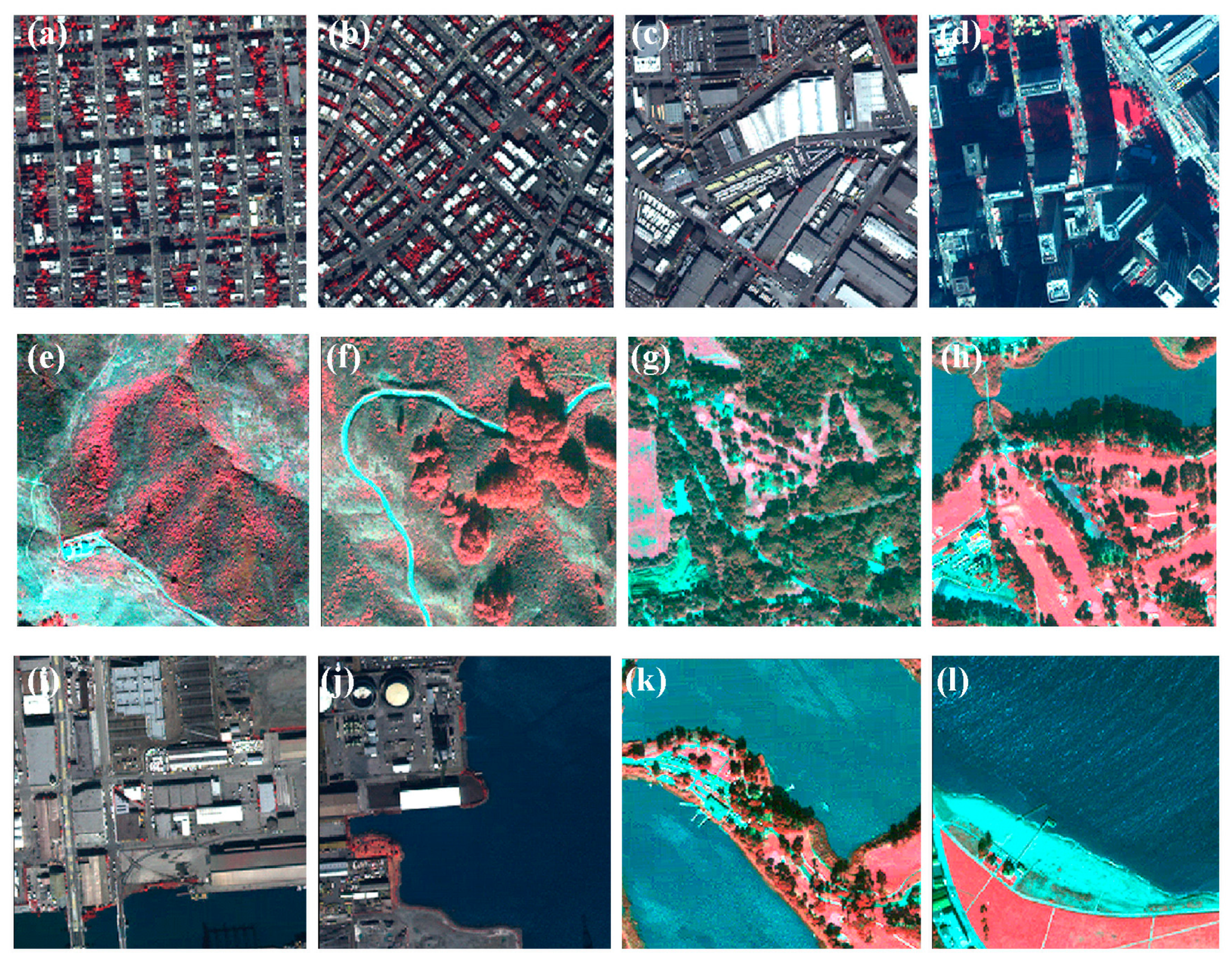
3.1. Test Images
A Quickbird image was obtained from IGARSS 2012. The image was acquired on 11 November 2007, and covers the city of San Francisco, CA, USA. The spatial resolution of the multi-spectral image is 2.4 m. We selected the 12 subset images shown in Figure 1a–l with uniform sizes of 256 × 256 pixels. The test images can be classified into three categories: Figure 1a–d urban areas; Figure 1e–g rural areas; and Figure 1h–l harbor areas.
3.2. Degradation Methods
The methods employed to simulate the distortion of the test images are introduced as follows.
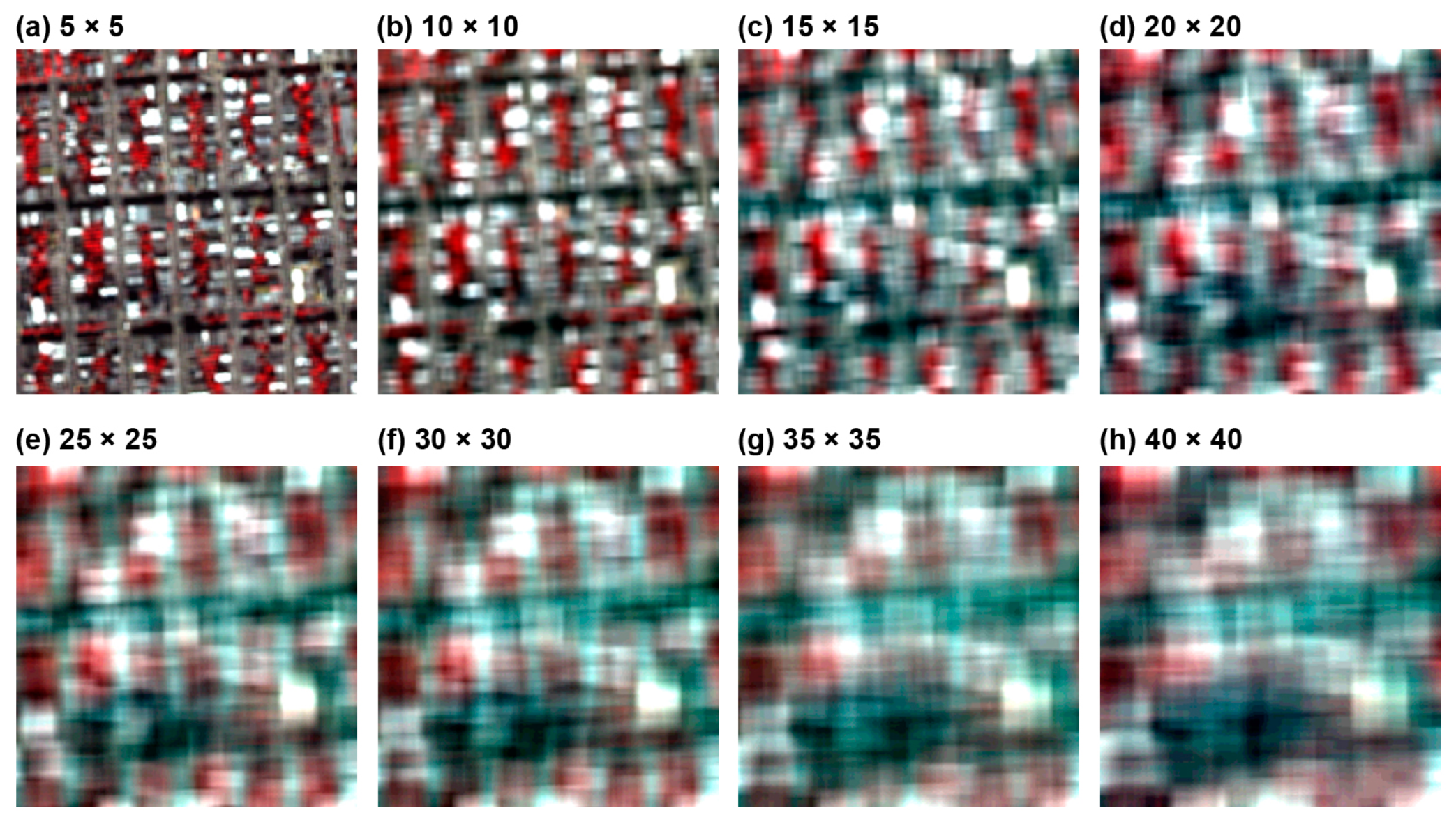
(a) Average filter degradation
Average filtering replaces each pixel value in an image with the average value of its neighbors and itself. Average filtering is a kind of convolution filter. Like other convolution filters, it is based on a kernel, which represents the shape and size of the neighborhood to be sampled when calculating the average. In this paper, the kernel is a square matrix with an edge dimension ranging from 1 to 40 pixels in increments of 1. Average filtering provides image distortion that is representative of spatial resolution degradation.
To allow for a visual interpretation of the relative effects on image quality obtained after the application of average filter degradation in terms of monotonicity, we present Figure 1a subjected to average filter degradation for kernels with an edge dimension ranging from 5 to 40 pixels in increments of 5, as shown in Figure 2.
We note from Figure 2 that the image quality obviously decreased with increasing kernel size. Visually, the differences in the image degradation between level 5 and level 20 are much greater than between level 25 and level 40, where the latter levels present only relatively slight differences. These images show that the average filter degradation has a decreasing effect on image quality with an increasing coarseness of spatial resolution.
(b) Gaussian white noise degradation
Gaussian white noise with a probability density function satisfying a normal distribution was added into images. Here, the mean value of the noise was set to 0 and the variance ranged from 0.0005 to 0.02 in increments of 0.0005.
We present Figure 1a subjected to Gaussian white noise degradation with variance ranging from 0.0025 to 0.02 in increments of 0.0025, as shown in Figure 3.
We note from Figure 3 that the image quality obviously decreased with increasing variance of Gaussian white noise. The street in Figure 1a is heavily blurred by the noise with variance larger than 0.005. The building and trees are mixed when the variance of the noise reaches 0.0125. These images show that the Gaussian white noise has a decreasing effect on image quality with an increasing variance of noise.
(c) Linear motion degradation
The images were convolved with a filter that simulates the linear motion of a camera moving by m pixels at an angle of n degrees counterclockwise from the horizontal direction to the right. In this paper, n is set to 45° and m ranges from 1 to 40 pixels in increments of 1.
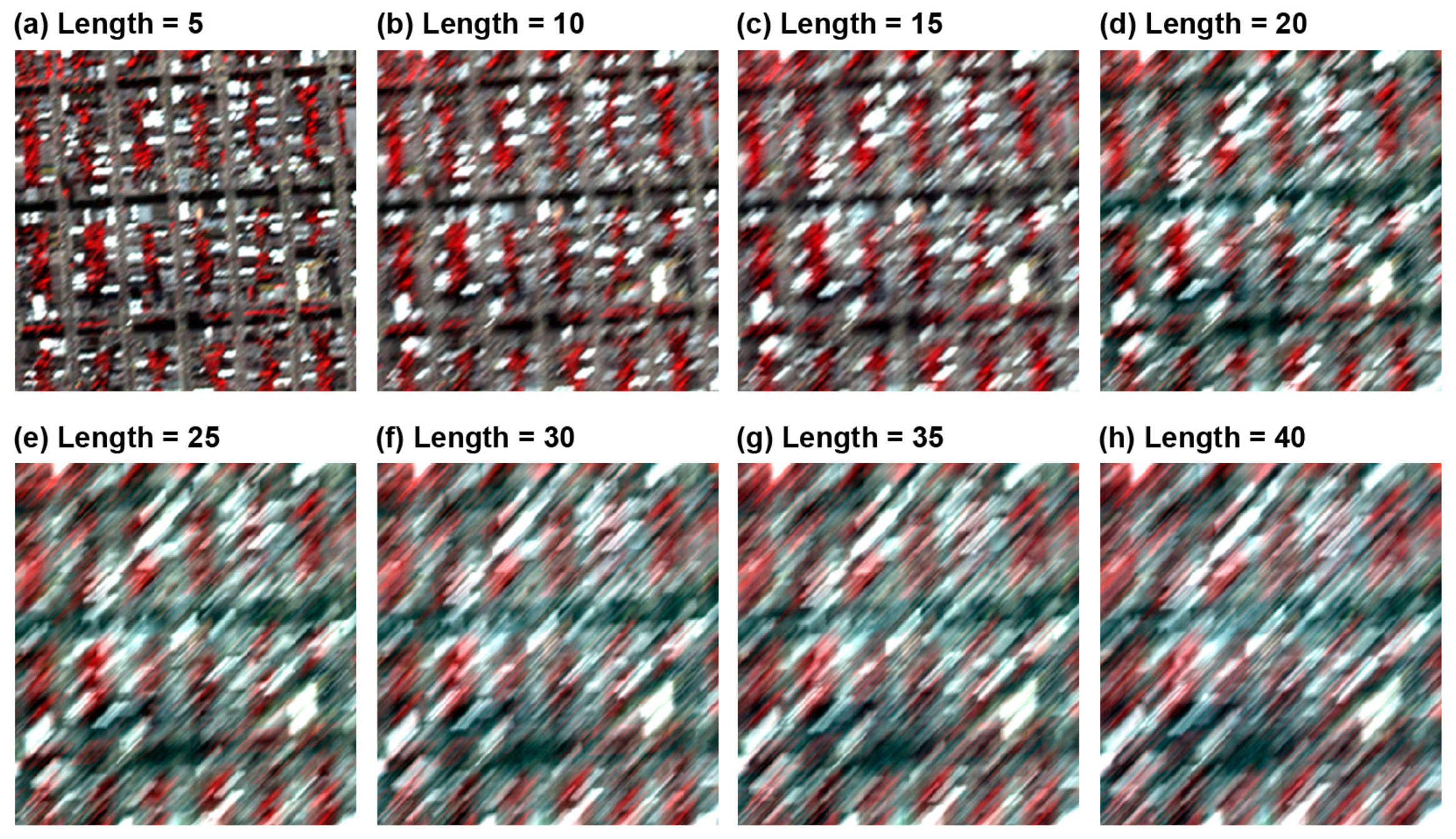
We present Figure 1a subjected to linear motion degradation with pixels at an angle of 45° ranging from 5 to 40 in increments of 5, as shown in Figure 4.
We note from the Figure 4 that the image quality obviously decreased with increasing length size. It is difficult to distinguish land covers when pixel length reaches length size of 25. Similar to the results of average filter degradation, the differences in the image degradation between length size of 5 and 20 are much greater than between length size of 25 and 40, where the latter length sizes present only relatively slight differences.
4. Statistical Analysis of Evaluation Results
Owing to the 40 levels for each of the three classes of distortion investigated, 120 degraded images are obtained for each original image. Therefore, a total of 1440 (12 × 120) images were employed as samples for evaluation. As discussed in a past study [6], a good IQM must provide good prediction accuracy, prediction monotonicity, and prediction consistency. The prediction accuracy was determined by one-way analysis of variance (ANOVA) test, the prediction monotonicity was determined by the scatter plot of the degradation level and the IQM values, and the prediction consistency was determined by the Pearson linear correlation coefficient. The IQMs passed the three tests were determined to be robust. As the redundancy may exists, the robust IQMs were then classified into various components (or clusters) using factor analysis (FA), and the IQM with the highest loading coefficient was selected as the representative metric for each component.
4.1. Robustness of No-Reference Image Quality Metrics for Remote Sensing Images
4.1.1. Prediction Accuracy
An objective IQM that provides good prediction accuracy is unaffected by image content. As such, the evaluation results of an IQM should be similar for equivalent degradation levels, regardless of the image content. One-way ANOVA was employed to evaluate the prediction accuracy. One-way ANOVA weighs a hypothesis that each sample is drawn from the same underlying probability distribution against an alternative hypothesis that underlying probability distributions are not the same for all samples. The hypotheses for the comparison of independent groups are
where H0 denotes that the mean values of all groups are equal, and H1 denotes that the mean values of two or more groups are not equal. The null hypothesis indicates that no significant difference exists between the sample means. A high value for the F test indicates that the null hypothesis is rejected. Thus, any test results with an F test value larger than critical value would be significant, and the null hypothesis is rejected. This is used to determine whether the variation in the scores of IQMs arises predominantly from image degradation or from the image content. The metrics that are sensitive to image content are not suitable for objective image quality assessment.
4.1.2. Prediction Monotonicity
To be consistent with visual inspection, an IQM should demonstrate a monotonic dependence on the level of degradation of an image and exhibit small variations for different images with equivalent levels of degradation [34]. A scatter plot is used to test the prediction monotonicity.
4.1.3. Prediction Consistency
The evaluation results of an IQM are judged according to how well the results correlate with the degradation level. The Pearson linear correlation coefficient (PLCC) is employed to quantitatively measure the correlation between image degradation levels and the results of NR metrics. The PLCC is defined as
where Level(i) is the degradation level of the ith image, Levelavg is the average degradation level of all images, NR(i) is the evaluation results of an NR metric for the ith image, and NRavg is the average evaluation results of an NR metric for all images.
4.2. Cluster Analysis of Robust Image Quality Metrics
As there may exist redundancy in robust IQMs, factor analysis (FA) based on principal component analysis (PCA) was employed to group similar IQMs into fewer factors. To verify the appropriateness of FA for this study, the Kaiser–Meyer–Olkin (KMO) measurement of sample adequacy and Bartlett’s test of sphericity were performed on the correlation matrix of IQMs. When the KMO was greater than 0.5, the sample was considered adequate for FA [35,36]. Bartlett’s test of sphericity tests the null hypothesis that the correlation matrix is an identity matrix. When this null hypothesis is rejected, the FA is appropriate for clustering robust IQMs. Each IQM is assumed to depend on a linear combination of the common factors, and the coefficients are known as loadings. Rotation was used to reorient the factor loadings so that the factors were more interpretable. The simplest case of rotation was an orthogonal rotation (varimax) in which the angle between the reference axes of factors was maintained at 90°. This type of rotation was used with PCA. We performed FA on the metrics deemed robust for the different types of image degradation considered.
5. Results and Discussion
5.1. Results of Robustness Analysis
5.1.1. Prediction Accuracy
The results of one-way ANOVA testing for 21 IQMs based on 40 degradation levels for each type of degradation applied to the 12 sample images are listed in Table 1. The abbreviations used in Table 1 are defined in Section 2.
The critical value of the F test for each IQM in Table 1 is 1.427. The values in grey in Table 1 therefore do not reject the null hypothesis, and, thus, the corresponding IQMs were affected by image content more than by the image degradation level. For average filter degradation, all of the IQMs were robust for different image contents. For Gaussian noise degradation, the results of EM were affected by image content. For linear motion degradation, the results of BIQAA, BLIINDS-II, EM, and KM were affected by image content. The metrics that are sensitive to image content are not suitable for image quality assessment.
5.1.2. Prediction Monotonicity
The scatter plot results for the 21 IQMs based on 40 degradation levels for each type of degradation applied to the 12 sample images are presented and discussed in this subsection.
(a) Average filter degradation
The scatter plots for the 21 IQMs based on the 40 levels of average filter degradation applied to the 12 sample images are presented in Figure 5.
The IQMs were classified into four groups according to their degree of monotonicity, as Decreasing, Increasing, Fluctuating, and Unchanging. The four groups are given as follows:
For the Decreasing group, the evaluation results sharply decreased over the first 10 degradation levels, and changed little for the remaining 30 degradation levels, which are consistent with a visual inspection of Figure 2. For the Increasing group, the evaluation results were negatively correlated with the degradation levels. For the Fluctuating group, BIQI, BLIINDS-II, BRISEQ, CPBD, JNBM, and QAC were trained for a specific digital image dataset, which produced fluctuating evaluation results for different image contents. Therefore, it can be concluded that the results of the training-based IQMs are highly dependent on the training samples employed, and cannot be directly applied for the image quality evaluation of remote sensing images. For the other IQMs in this group, BM was proposed based on subjective tests and psychophysics functions and was limited to the specific images. KM measures the depth of focus, while Quickbird images are obtained with a uniform depth of focus. SM measures the asymmetry of the data, which is not a suitable metric for remote sensing images. The Unchanging group provided equivalent evaluations for all images regardless of the degradation level. DM was designed to measure the effect of frequency distortion, and is therefore not sensitive to average filter degradation. MM measures the mean pixel value of the image, which is unaffected by average filter operations, such that the results of MM remained unchanged with increasing degradation.
(b) Gaussian white noise degradation
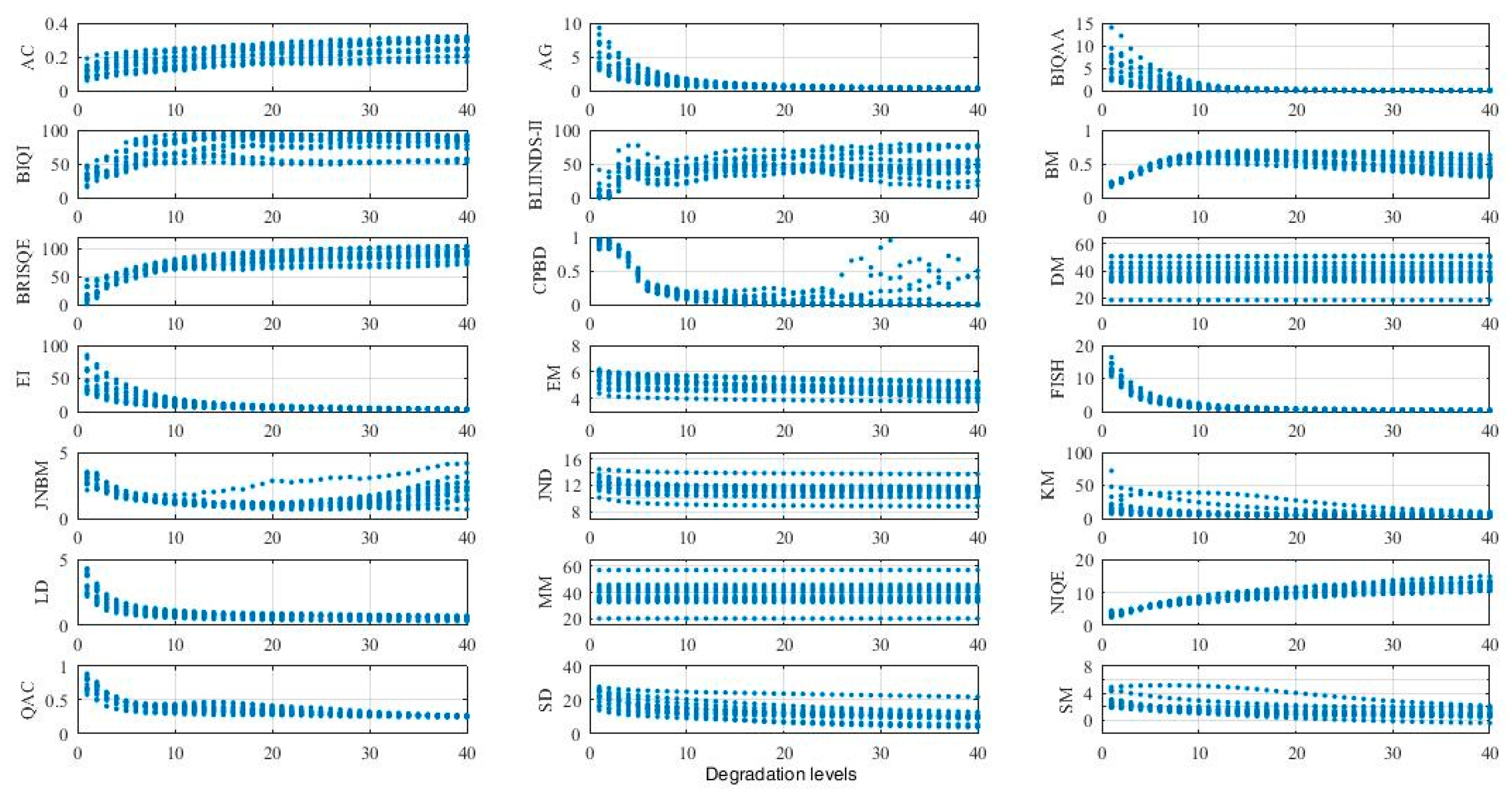
The scatter plots for the 21 IQMs based on the 40 levels of Gaussian white noise degradation applied to the 12 sample images are presented in Figure 6.
The IQMs were classified into three groups according to their degree of monotonicity, as Decreasing, Increasing, and Fluctuating. The three groups are given as follows:
For the Decreasing group, the evaluation results of AC, BM, KM, and SM demonstrate a decreasing trend with increasing degradation, while, with respect to the level of average filter degradation, the results of AC demonstrated an increasing trend and the results of BM, KM, and SM fluctuated. The evaluation results of the Increasing group demonstrate an increasing trend with increasing degradation. Meanwhile, the results of AG, EI, FISH, JND, LD, and SD demonstrated a decreasing trend with increasing average filter degradation, the results of BIQI fluctuated with respect to the level of average filter degradation, and the results of DM and MM were unchanging with respect to the level of average filter degradation. The members of the Fluctuating group here largely coincide with those of the Fluctuating group obtained for average filter degradation. For those members not in the same group, EM demonstrated unchanging results and the results of NIQE fluctuated with respect to the level of average filter degradation.
(c) Linear motion degradation
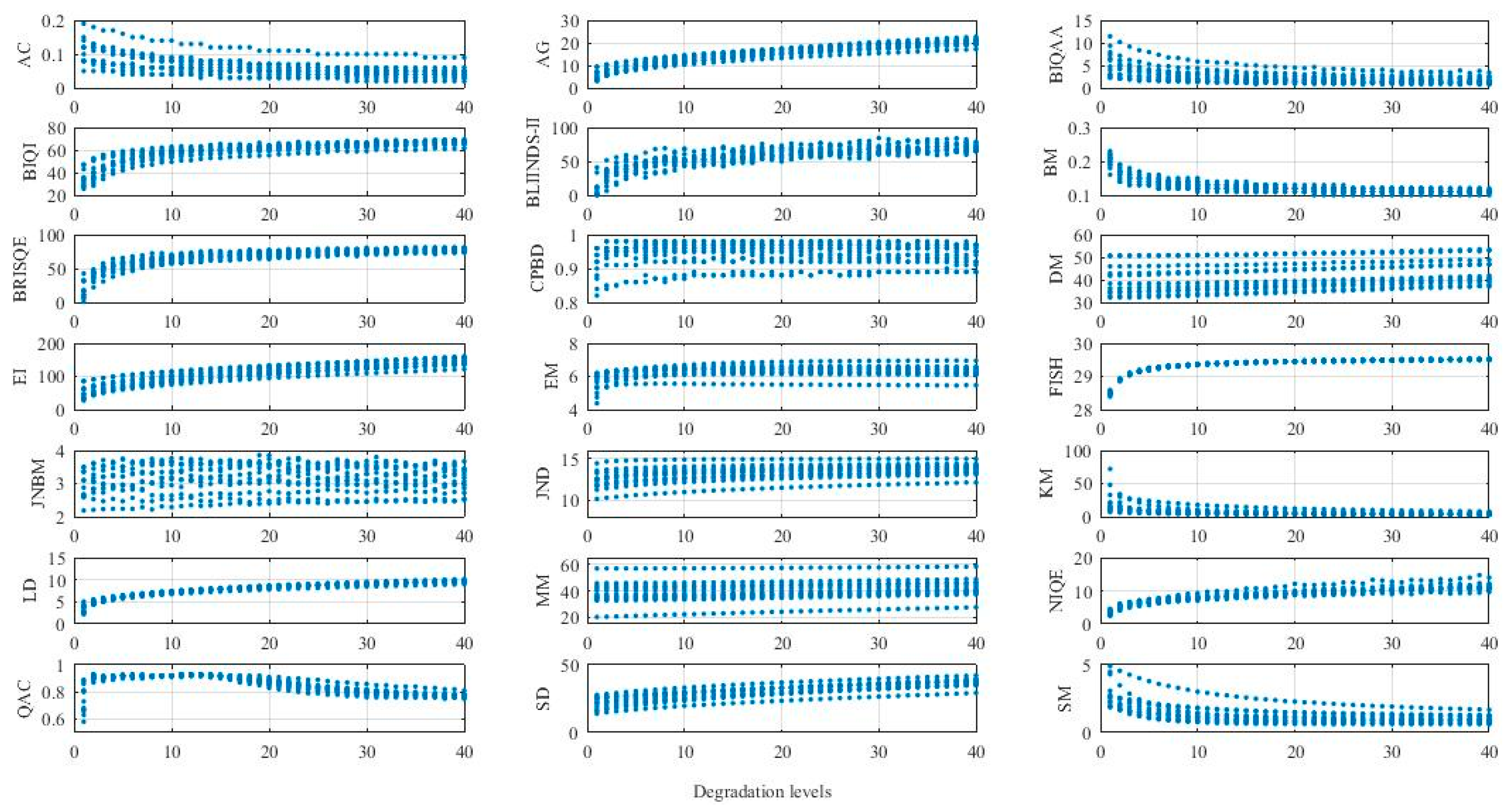
The scatter plots for the 21 IQMs based on the 40 levels of linear motion degradation applied to the 12 sample images are presented in Figure 7.
The IQMs were classified into four groups according to their degree of monotonicity. The four groups are given as follows:
The results of linear motion degradation were very similar to the results obtained for average filter degradation. We note that the results of BIQAA and NIQE demonstrate a fluctuating trend with respect to the level of linear motion degradation while having, respectively, demonstrated decreasing and increasing trends with respect to the level of average filter degradation. The results of BM demonstrate an increasing trend with increasing linear motion degradation while having demonstrated a fluctuating trend with respect to the level of average filter degradation.
5.1.3. Prediction Consistency
The PLCC values between degradation levels for the three types of degradation and the IQM evaluation results for the 12 sample images are listed in Table 2. The results marked in gray in the table reside below the 0.05 confidence level, therefore indicating that the IQM fails to fulfill the requirements of prediction consistency.
5.1.4. Summary of the Robustness of Image Quality Metrics
We summarized the evaluation results for the 21 IQMs based on their fulfillment of the requirements of prediction accuracy, prediction monotonicity, and prediction consistency in Table 3.
The IQMs fulfilling the requirements of prediction accuracy, prediction monotonicity, and prediction consistency for the three types of degradation are summarized in Table 4.
5.2. Factor Analysis of Robust Image Quality Metrics
The robust IQMs listed in Table 4 were subjected to FA to determine the representative IQM for each type of degradation. The KMO and Bartlett’s test results are listed in Table 5. From Table 5, we note that FA is appropriate for the intended study.
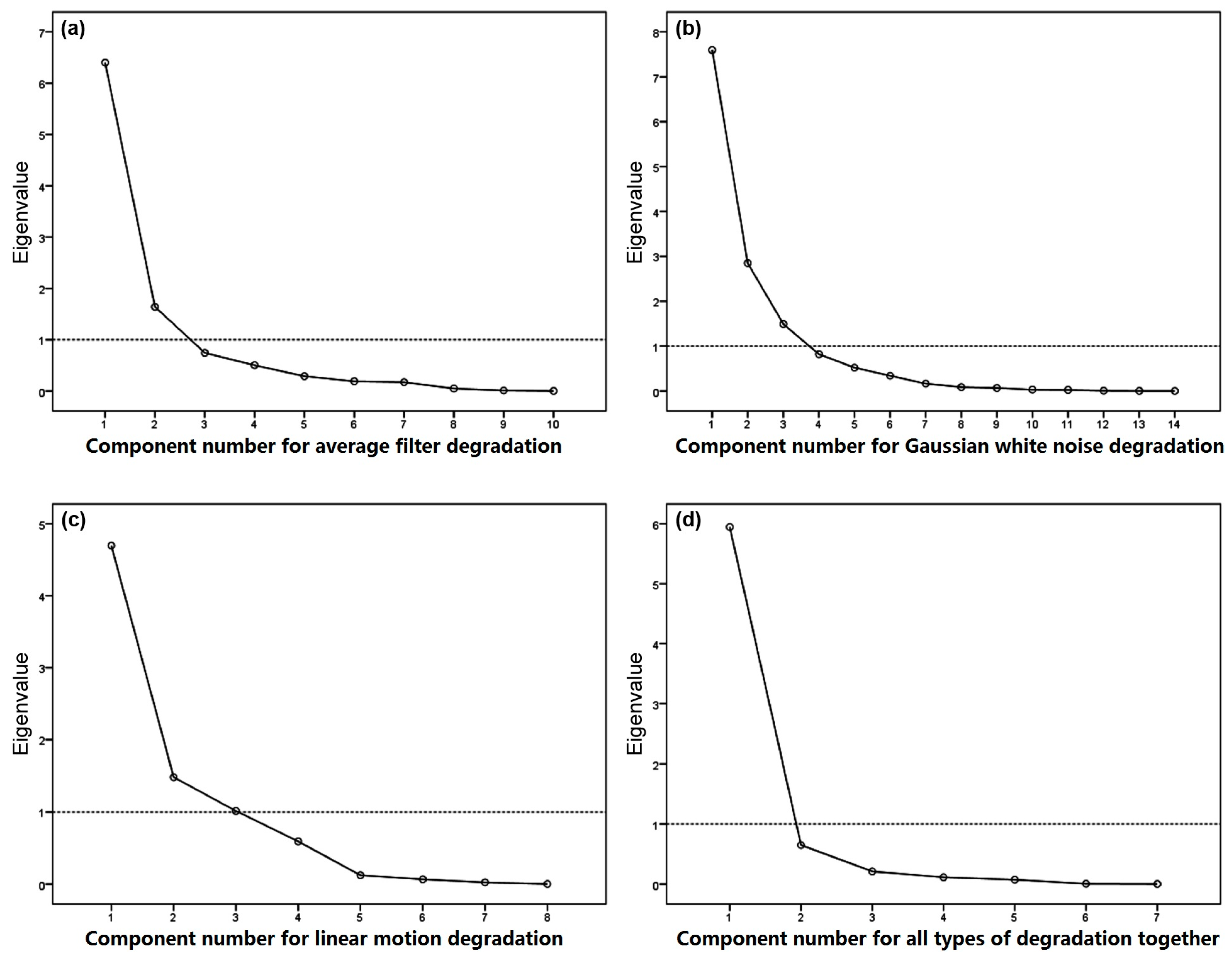
The eigenvalues of the robust IQMs (i.e., components) listed in Table 4 are plotted in Figure 8 for all types of degradation. The eigenvalue provides a measure of the significance of the component. Eigenvalues greater than or equal to 1.0 are considered significant [37]. The number of components equal to the number of IQMs. From Figure 8, we note that two components are retained for average filter degradation, three for Gaussian white noise degradation, three for linear motion degradation, and one for all types of degradation together.
Table 6, Table 7, Table 8 and Table 9 present the component loading matrix for each type of degradation after conducting orthogonal rotation. The loading value was the correlation coefficient between IQMs and retained components. For each IQM, the level of importance of an IQM on a component increases with increasing loading value.
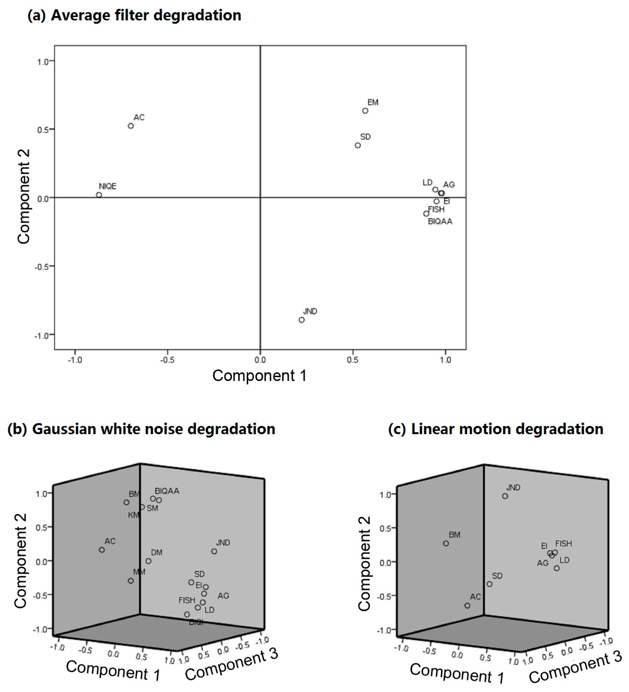
The IQMs clustered in two-dimensional and three-dimensional component space are shown in Figure 9. The IQM with the highest loading value on a component was selected as the representative IQM for a given type of degradation. The results are summarized as follows:
- Average filter degradationComponent 1: EI, AG, FISH, LD, BIQAA, NIQE, AC, SD.Component 2: JND, EM.
From the perspective of the spatial resolution of an image, the results suggest EI and JND for evaluating the quality of an image:
- Gaussian white noise degradationComponent 1: EI, AG, LD, SD, AC.Component 2: BIQAA, SM, BM, BIQI, KM, FISH.Component 3: MM, JND, DM.
The results suggest EI, BIQAA, and MM for evaluating the quality of an image:
- Linear motion degradationComponent 1: LD, AG, FISH, EI, BM.Component 2: JND, AC.Component 3: SD.
The results suggest LD, JND, and SD for evaluating the quality of an image:
- All degradation typesComponent 1: EI, LD, AG, FISH, SD, AC, JND.
EI is suggested for evaluating the quality of an image when the type of degradation is unknown.
6. Conclusions
In this paper, 21 objective NR IQMs were reviewed and evaluated for Quickbird images with urban, rural, and harbor contents subjected to 40 different levels of average filter, Gaussian white noise, and linear motion degradation. The experimental results provide a number of suggestions. (1) Different IQMs performed differently for different image contents and different types of image degradation. Generally, the effect of the degradation type was stronger than that of the image content on the evaluation results. (2) The same IQM can provide opposite dependences on the level of degradation for different degradation types, e.g., the evaluation results of AC demonstrated a decreasing trend with increasing Gaussian white noise degradation and an increasing trend with increasing average filter degradation, and the evaluation results of AG, EI, FISH, JND, LD, and SD demonstrated increasing trends with increasing Gaussian white noise degradation and decreasing trends with increasing average filter degradation. (3) An IQM that performed well with one type of degradation may not perform well with another type, e.g., the evaluation results of BIQAA fluctuated with respect to the level of linear motion degradation and demonstrated a decreasing trend with increasing average filter degradation, the evaluation results of BM demonstrated an increasing trend with increasing linear motion degradation and fluctuated with respect to the level of average filter degradation, and the evaluation results of NIQE fluctuated with respect to the level of linear motion degradation and increased with increasing average filter degradation. (4) The general results of clustering provided suggestions for representative IQMs most appropriate for the different types of degradation. For average filter degradation, EI and JND for evaluating the quality of an image. For Gaussian white noise degradation, EI, BIQAA, and MM for evaluating the quality of an image. For linear motion degradation, LD, JND, and SD for evaluating the quality of an image. (5) For image quality assessment without knowledge of the degradation type, EI was suggested for evaluating the quality of an image.
Acknowledgments
This work was supported by a grant from 973 project in China (Grant #2012CB719901).
Author Contributions
Shuang Li conceived and designed the experiments; Zewei Yang performed the experiments; Shuang Li and Hongsheng Li analyzed the data; and Shuang Li wrote the paper.
Conflicts of Interest
The authors declare no conflict of interest.
References
- Cohen, E.; Yitzhaky, Y. No-reference assessment of blur and noise impacts on image quality. Signal Image Video Process. 2010, 4, 289–302. [Google Scholar] [CrossRef]
- Wang, Z.; Bovik, A.C. Modern image quality assessment. Synth. Lect. Image Video Multimed. Process. 2006, 2, 1–156. [Google Scholar] [CrossRef]
- Ferzli, R.; Karam, L.J. A no-reference objective image sharpness metric based on the notion of just noticeable blur (JNB). IEEE Trans. Image Process. 2009, 18, 717–728. [Google Scholar] [CrossRef] [PubMed]
- Chandler, D.M. Seven challenges in image quality assessment: Past, present, and future research. ISRN Signal Process. 2013, 2013, 905685. [Google Scholar] [CrossRef]
- Wang, Z.; Bovik, A.C. Mean squared error: Love it or leave it? A new look at signal fidelity measures. IEEE Signal Process. Mag. 2009, 26, 98–117. [Google Scholar] [CrossRef]
- Ismail, A.; Bulent, S.; Sayood, K. Statistical evaluation of image quality measures. J. Electron. Imaging 2002, 11, 206–223. [Google Scholar]
- Ong, E.; Lin, W.; Lu, Z.; Yao, S.; Yang, X.; Jiang, L. No-reference JPEG-2000 image quality metric. In Proceedings of the International Conference on Multimedia and Expo, Baltimore, MD, USA, 6–9 July 2003; pp. 545–548. [Google Scholar]
- Cohen, E.; Yitzhaky, Y. Blind image quality assessment considering blur, noise, and JPEG compression distortions. In Proceedings of the Applications of Digital Image Processing XXX, San Diego, CA, USA, 26 August 2007. [Google Scholar]
- Wang, Z.; Bovik, A.C.; Sheikh, H.R.; Simoncelli, E.P. Image quality assessment: From error visibility to structural similarity. IEEE Trans. Image Process. 2004, 13, 600–612. [Google Scholar] [CrossRef] [PubMed]
- Wang, Z.; Simoncelli, E.P. Reduced-reference image quality assessment using a wavelet-domain natural image statistic model. In Proceedings of the Society of Photo-optical Instrumentation Engineers, Human Vision and Electronic Imaging, San Jose, CA, USA, 17–20 January 2005; pp. 149–159. [Google Scholar]
- Carnec, M.; Le Callet, P.; Barba, D. Objective quality assessment of color images based on a generic perceptual reduced reference. Signal Process. Image Commun. 2008, 23, 239–256. [Google Scholar] [CrossRef]
- Eskicioglu, A.M.; Fisher, P.S. Image quality measures and their performance. IEEE Trans. Commun. 1995, 43, 2959–2965. [Google Scholar] [CrossRef]
- Chen, M.J.; Bovik, A.C. No-reference image blur assessment using multiscale gradient. EURASIP J. Image Video Process. 2011. [Google Scholar] [CrossRef]
- Ciancio, A.; da Costa, A.T.; da Silva, E.A.; Said, A.; Samadani, R.; Obrador, P. No-reference blur assessment of digital pictures based on multifeature classifiers. IEEE Trans. Image Process. 2011, 20, 64–75. [Google Scholar] [CrossRef] [PubMed]
- Shen, H.; Zhao, W.; Yuan, Q.; Zhang, L. Blind Restoration of Remote Sensing Images by a Combination of Automatic Knife-Edge Detection and Alternating Minimization. Remote Sens. 2014, 6, 7491–7521. [Google Scholar] [CrossRef]
- Rodger, J.A. Toward reducing failure risk in an integrated vehicle health maintenance system: A fuzzy multi-sensor data fusion Kalman filter approach for IVHMS. Expert Syst. Appl. 2012, 3, 9821–9836. [Google Scholar] [CrossRef]
- Sazzad, Z.P.; Kawayoke, Y.; Horita, Y. No reference image quality assessment for JPEG2000 based on spatial features. Signal Process. Image Commun. 2008, 23, 257–268. [Google Scholar] [CrossRef]
- Yang, X.H.; Jing, Z.L.; Liu, G.; Hua, L.Z.; Ma, D.W. Fusion of multi-spectral and panchromatic images using fuzzy rule. Commun. Nonlinear Sci. Numer. Simul. 2007, 12, 1334–1350. [Google Scholar] [CrossRef]
- Moorthy, A.K.; Bovik, A.C. A two-step framework for constructing blind image quality indices. IEEE Signal Process. Lett. 2010, 17, 513–516. [Google Scholar] [CrossRef]
- Gabarda, S.; Cristóbal, G. Blind image quality assessment through anisotropy. JOSA A 2007, 24, B42–B51. [Google Scholar] [CrossRef] [PubMed]
- Saad, M.A.; Bovik, A.C.; Charrier, C. A DCT statistics-based blind image quality index. IEEE Signal Process. Lett. 2010, 17, 583–586. [Google Scholar] [CrossRef]
- Crete, F.; Dolmiere, T.; Ladret, P.; Nicolas, M. The blur effect: Perception and estimation with a new no-reference perceptual blur metric. In Proceedings of the Human Vision and Electronic Imaging XII, San Jose, CA, USA, 28 January 2007. [Google Scholar]
- Mittal, A.; Moorthy, A.; Bovik, A. No-reference image quality assessment in the spatial domain. IEEE Trans. Image Process. 2012, 21, 4695–4708. [Google Scholar] [CrossRef] [PubMed]
- Narvekar, N.D.; Karam, L.J. A no-reference image blur metric based on the cumulative probability of blur detection (CPBD). IEEE Trans. Image Process. 2011, 20, 2678–2683. [Google Scholar] [CrossRef] [PubMed]
- Damera-Venkata, N.; Kite, T.D.; Geisler, W.S.; Evans, B.L.; Bovik, A.C. Image quality assessment based on a degradation model. IEEE Trans. Image Process. 2000, 9, 636–650. [Google Scholar] [CrossRef] [PubMed]
- Karathanassi, V.; Kolokousis, P.; Ioannidou, S. A comparison study on fusion methods using evaluation indicators. Int. J. Remote Sens. 2007, 28, 2309–2341. [Google Scholar] [CrossRef]
- Vu, P.V.; Chandler, D.M. A fast wavelet-based algorithm for global and local image sharpness estimation. IEEE Signal Process. Lett. 2012, 19, 423–426. [Google Scholar] [CrossRef]
- Yang, X.; Ling, W.; Lu, Z.; Ong, E.P.; Yao, S. Just noticeable distortion model and its applications in video coding. Signal Process. Image Commun. 2005, 20, 662–680. [Google Scholar] [CrossRef]
- Wei, Z.; Ngan, K.N. Spatio-temporal just noticeable distortion profile for grey scale image/video in DCT domain. IEEE Trans. Circuits Syst. Video Technol. 2009, 19, 337–346. [Google Scholar]
- Caviedes, J.; Oberti, F. A new sharpness metric based on local kurtosis, edge and energy information. Signal Process. Image Commun. 2004, 19, 147–161. [Google Scholar] [CrossRef]
- Zhang, J.; Ong, S.H.; Le, T.M. Kurtosis-based no-reference quality assessment of JPEG2000 images. Signal Process. Image Commun. 2011, 26, 13–23. [Google Scholar] [CrossRef]
- Mittal, A.; Soundararajan, R.; Bovik, A.C. Making a “Completely Blind” Image Quality Analyzer. IEEE Signal Process. Lett. 2013, 20, 209–212. [Google Scholar] [CrossRef]
- Xue, W.; Zhang, L.; Mou, X. Learning without Human Scores for Blind Image Quality Assessment. In Proceedings of the 2013 IEEE Conference on Computer Vision and Pattern Recognition (CVPR), Portland, OR, USA, 23–28 June 2013. [Google Scholar]
- Feichtenhofer, C.; Fassold, H.; Schallauer, P. A Perceptual Image Sharpness Metric Based on Local Edge Gradient Analysis. IEEE Signal Process. Lett. 2013, 20, 379–382. [Google Scholar] [CrossRef]
- Li, S.; Li, Z.; Gong, J. Multivariate statistical analysis of measures for assessing the quality of image fusion. Int. J. Image Data Fusion 2010, 1, 47–66. [Google Scholar] [CrossRef]
- MacCallum, R. A comparison of factor analysis programs in SPSS, BMDP, and SAS. Psychometrika 1983, 48, 223–231. [Google Scholar] [CrossRef]
- Kim, J.O.; Mueller, C.W. Introduction to Factor Analysis: What It Is and How to Do It; Sage: Thousand Oaks, CA, USA, 1978. [Google Scholar]
Figure 1.
Test Quickbird images: (a–d) urban areas; (e–g) rural areas; (h–l) harbor areas.

Figure 2.
Average filter degradation for the image in Figure 1a.
Figure 2.
Average filter degradation for the image in Figure 1a.

Figure 3.
Gaussian white noise degradation for the image in Figure 1a.
Figure 3.
Gaussian white noise degradation for the image in Figure 1a.
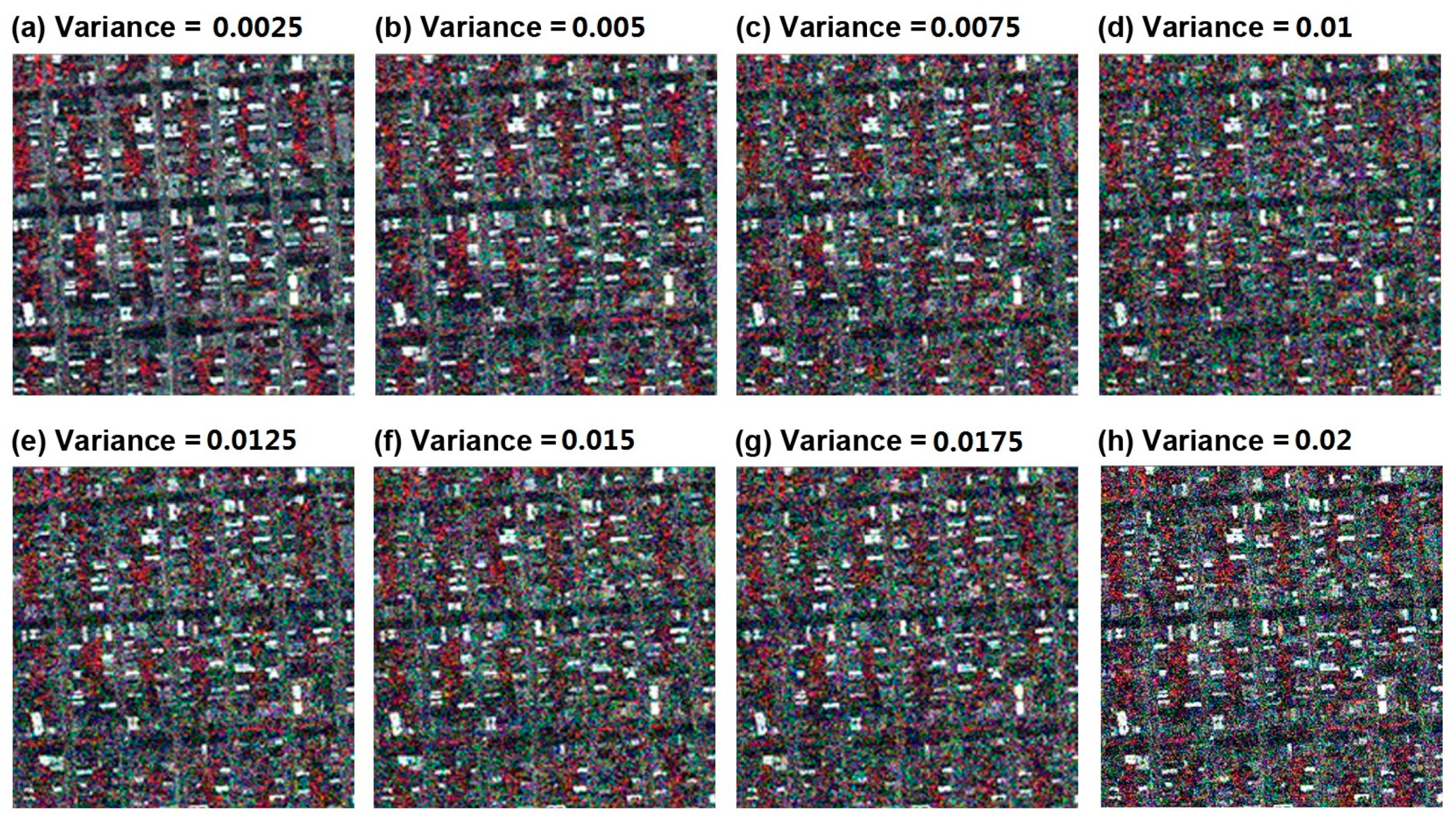
Figure 4.
Linear motion degradation for the image in Figure 1a.
Figure 4.
Linear motion degradation for the image in Figure 1a.

Figure 5.
Scatter plot of evaluation results for average filter degradation.

Figure 6.
Scatter plots of evaluation results for Gaussian white noise degradation.

Figure 7.
Scatter plots of evaluation results for linear motion degradation.
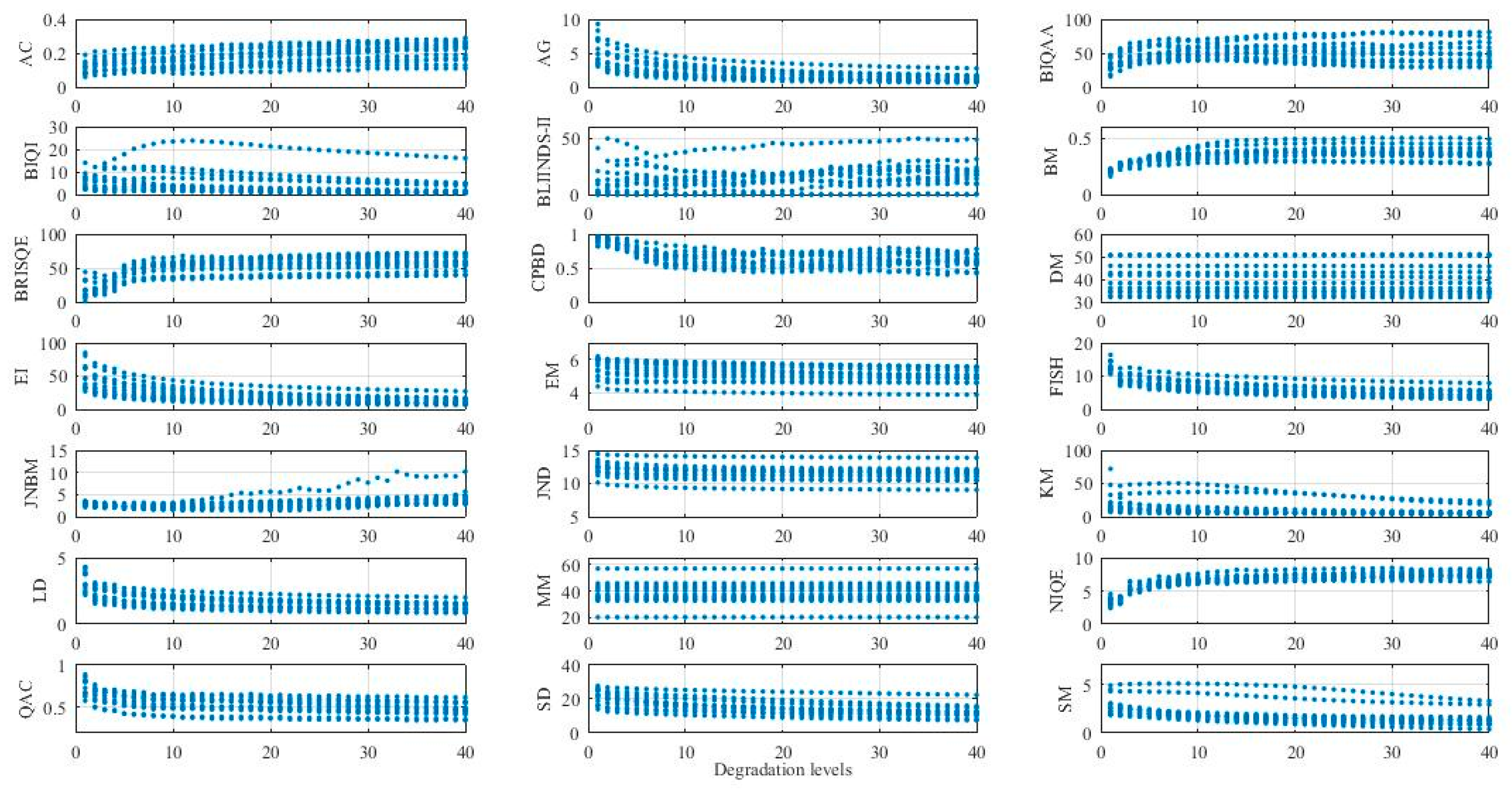
Figure 8.
Scatter plots of the eigenvalues for all components with respect to each degradation type.
Figure 8.
Scatter plots of the eigenvalues for all components with respect to each degradation type.

Figure 9.
Clustering of image quality metrics in two-dimensional and three-dimensional space.


Table 1.
One-way ANOVA test results for different types of degradation.
| Average | Gaussian | Motion | |
|---|---|---|---|
| AC | 36.37 | 38.2 | 36.67 |
| AG | 36.47 | 89.2 | 13.46 |
| BIQAA | 24.82 | 7.13 | 0.5 |
| BIQI | 13.34 | 112.48 | 3.54 |
| BLIINDS-II | 7.62 | 47.11 | 0.6 |
| BM | 32.8 | 37.53 | 34.63 |
| BRISQE | 63.34 | 123.48 | 14.42 |
| CPBD | 36.78 | 28.42 | 31.03 |
| DM | 3.7 | 5.41 | 3.68 |
| EI | 40.37 | 66.11 | 11.15 |
| EM | 2.49 | 0.59 | 1.21 |
| FISH | 1246.83 | 517.63 | 26.63 |
| JNBM | 16.11 | 6.6 | 4.78 |
| JND | 4.85 | 13.48 | 5.01 |
| KM | 3.17 | 7.67 | 1.14 |
| LD | 33.9 | 63.29 | 33.9 |
| MM | 3.84 | 5.47 | 3.84 |
| NIQE | 57.37 | 42.77 | 18.21 |
| QAC | 35.04 | 29.49 | 32.21 |
| SD | 5.65 | 31.38 | 5.14 |
| SM | 8.66 | 16.59 | 5.59 |
Table 2.
PLCC values between degradation levels and image qualities.
| Average | Gaussian | Motion | |
|---|---|---|---|
| AC | 0.670 | −0.744 | 0.463 |
| AG | −0.664 | 0.917 | −0.594 |
| BIQAA | −0.595 | −0.473 | −0.193 |
| BIQI | 0.445 | 0.778 | 0.083 |
| BLIINDS-II | 0.374 | 0.755 | 0.181 |
| BM | 0.056 | 0.169 | 0.402 |
| BRISQE | 0.763 | 0.767 | 0.510 |
| CPBD | −0.536 | 0.045 | −0.435 |
| DM | −0.004 | 0.910 | 0 |
| EI | −0.690 | 0.351 | −0.596 |
| EM | −0.425 | 0.192 | −0.232 |
| FISH | −0.704 | 0.736 | −0.776 |
| JNBM | −0.011 | 0.018 | 0.440 |
| JND | −0.193 | −0.701 | −0.166 |
| KM | −0.420 | −0.481 | −0.279 |
| LD | −0.617 | −0.538 | −0.553 |
| MM | 0.001 | 0.159 | 0 |
| NIQE | 0.886 | 0.865 | 0.686 |
| QAC | −0.759 | 0.873 | −0.425 |
| SD | −0.519 | 0.774 | −0.481 |
| SM | −0.467 | −0.485 | −0.341 |
Table 3.
Summary of test results, where PA denotes prediction accuracy, PM denotes prediction monotonicity, and PC denotes prediction consistency. Meanwhile, the symbol √ indicates that an IQM fulfills the requirements for a given criterion, and the symbol × indicates that it does not.
Table 3.
Summary of test results, where PA denotes prediction accuracy, PM denotes prediction monotonicity, and PC denotes prediction consistency. Meanwhile, the symbol √ indicates that an IQM fulfills the requirements for a given criterion, and the symbol × indicates that it does not.
| Average | Gaussian | Motion | |||||||
|---|---|---|---|---|---|---|---|---|---|
| PA | PM | PC | PA | PM | PC | PA | PM | PC | |
| AC | √ | √ | √ | √ | √ | √ | √ | √ | √ |
| AG | √ | √ | √ | √ | √ | √ | √ | √ | √ |
| BIQAA | √ | √ | √ | √ | √ | √ | × | × | √ |
| BIQI | √ | × | √ | √ | √ | √ | √ | × | × |
| BLIINDS-II | √ | × | √ | √ | × | √ | × | × | √ |
| BM | √ | × | × | √ | √ | √ | √ | √ | √ |
| BRISQE | √ | × | √ | √ | × | √ | √ | × | √ |
| CPBD | √ | × | √ | √ | × | × | √ | × | √ |
| DM | √ | × | × | √ | √ | √ | √ | × | × |
| EI | √ | √ | √ | √ | √ | √ | √ | √ | √ |
| EM | √ | √ | √ | × | × | √ | × | √ | √ |
| FISH | √ | √ | √ | √ | √ | √ | √ | √ | √ |
| JNBM | √ | × | × | √ | × | × | √ | × | √ |
| JND | √ | √ | √ | √ | √ | √ | √ | √ | √ |
| KM | √ | × | √ | √ | √ | √ | × | × | √ |
| LD | √ | √ | √ | √ | √ | √ | √ | √ | √ |
| MM | √ | × | × | √ | √ | √ | √ | × | × |
| NIQE | √ | √ | √ | √ | × | √ | √ | × | √ |
| QAC | √ | × | √ | √ | × | √ | √ | × | √ |
| SD | √ | √ | √ | √ | √ | √ | √ | √ | √ |
| SM | √ | × | √ | √ | √ | √ | √ | × | √ |
Table 4.
Robust IQMs for different degradations.
| Degradation | Robust IQMs |
|---|---|
| Average | AC, AG, BIQAA, EI, EM, FISH, JND, LD, NIQE, SD. |
| Gaussian | AC, AG, BIQAA, BIQI, BM, DM, EI, FISH, JND, KM, LD, MM, SD, SM. |
| Motion | AC, AG, BM, EI, FISH, JND, LD, SD. |
| Unknown | AC, AG, EI, FISH, JND, LD, SD. |
Table 5.
Results of KMO and Bartlett’s test.
| Average | Gaussian | Motion | All | ||
|---|---|---|---|---|---|
| KMO | 0.699 | 0.727 | 0.689 | 0.742 | |
| Bartlett’s test | Approximate chi squared | 8556.255 | 14,746.642 | 6576.038 | 25,101.243 |
| Freedom | 45 | 91 | 28 | 21 | |
| Significance | 0.000 | 0.000 | 0.000 | 0.000 | |
Table 6.
Rotated component matrix for average filter degradation.
| Component | ||
|---|---|---|
| 1 | 2 | |
| EI | 0.980 | 0.032 |
| AG | 0.975 | 0.032 |
| FISH | 0.951 | −0.028 |
| LD | 0.944 | 0.058 |
| BIQAA | 0.895 | −0.118 |
| NIQE | −0.871 | 0.019 |
| AC | −0.699 | 0.523 |
| SD | 0.526 | 0.382 |
| JND | 0.223 | −0.894 |
| EM | 0.566 | 0.634 |
Table 7.
Rotated component matrix for Gaussian white noise degradation.
| Component | |||
|---|---|---|---|
| 1 | 2 | 3 | |
| EI | 0.921 | −0.328 | 0.113 |
| AG | 0.880 | −0.431 | 0.101 |
| LD | 0.805 | −0.579 | 0.026 |
| SD | 0.787 | −0.245 | 0.293 |
| AC | −0.700 | 0.105 | 0.449 |
| BIQAA | −0.001 | 0.843 | −0.008 |
| SM | −0.251 | 0.813 | −0.212 |
| BM | −0.408 | 0.806 | 0.238 |
| BIQI | 0.518 | −0.787 | 0.018 |
| KM | −0.365 | 0.693 | −0.095 |
| FISH | 0.631 | −0.691 | −0.098 |
| MM | 0.169 | −0.190 | 0.952 |
| JND | 0.351 | −0.007 | −0.914 |
| DM | 0.401 | 0.107 | 0.834 |
Table 8.
Rotated component matrix for linear motion degradation.
| Component | |||
|---|---|---|---|
| 1 | 2 | 3 | |
| LD | 0.978 | −0.044 | 0.018 |
| AG | 0.967 | 0.157 | 0.126 |
| FISH | 0.960 | 0.190 | 0.037 |
| EI | 0.953 | 0.195 | 0.150 |
| BM | −0.595 | 0.246 | 0.593 |
| JND | −0.002 | 0.909 | −0.065 |
| AC | −0.588 | −0.748 | 0.059 |
| SD | 0.337 | −0.227 | 0.815 |
Table 9.
Rotated component matrix for all degradation types together.
| Component | |
|---|---|
| 1 | |
| EI | 0.984 |
| LD | 0.983 |
| AG | 0.980 |
| FISH | 0.964 |
| SD | 0.898 |
| AC | −0.888 |
| JND | 0.726 |
© 2017 by the authors. Licensee MDPI, Basel, Switzerland. This article is an open access article distributed under the terms and conditions of the Creative Commons Attribution (CC BY) license (http://creativecommons.org/licenses/by/4.0/).
Share and Cite
MDPI and ACS Style
Li, S.; Yang, Z.; Li, H. Statistical Evaluation of No-Reference Image Quality Assessment Metrics for Remote Sensing Images. ISPRS Int. J. Geo-Inf. 2017, 6, 133. https://0-doi-org.brum.beds.ac.uk/10.3390/ijgi6050133
AMA Style
Li S, Yang Z, Li H. Statistical Evaluation of No-Reference Image Quality Assessment Metrics for Remote Sensing Images. ISPRS International Journal of Geo-Information. 2017; 6(5):133. https://0-doi-org.brum.beds.ac.uk/10.3390/ijgi6050133
Chicago/Turabian StyleLi, Shuang, Zewei Yang, and Hongsheng Li. 2017. "Statistical Evaluation of No-Reference Image Quality Assessment Metrics for Remote Sensing Images" ISPRS International Journal of Geo-Information 6, no. 5: 133. https://0-doi-org.brum.beds.ac.uk/10.3390/ijgi6050133
Note that from the first issue of 2016, this journal uses article numbers instead of page numbers. See further details here.