Ranking the City: The Role of Location-Based Social Media Check-Ins in Collective Human Mobility Prediction

Abstract

Technological advances have led to an increasing development of data sources. Since the introduction of social networks, numerous studies on the relationships between users and their behaviors have been conducted. In this context, trip behavior is an interesting topic that can be explored via Location-Based Social Networks (LBSN). Due to the wide availability of various spatial data sources, the long-standing field of collective human mobility prediction has been revived and new models have been introduced. Recently, a parameterized model of predicting human mobility in cities, known as rank-based model, has been introduced. The model predicts the flow from an origin toward a destination using “rank” concept. However, the notion of rank has not yet been well explored. In this study, we investigate the potential of LBSN data alongside the rank concept in predicting human mobility patterns in Manhattan, New York City. For this purpose, we propose three scenarios, including: rank-distance, the number of venues between origin and destination, and a check-in weighted venue schema to compute the ranks. When trip distribution patterns are considered as a whole, applying a check-in weighting schema results in patterns that are approximately 10 percent more similar to the ground truth data. From the accuracy perspective, as the predicted numbers of trips are closer to real number of trips, the trip distribution is also enhanced by about 50 percent.

1. Introduction

Development of new data acquisition techniques has facilitated the study of human mobility patterns. Taking advantages of Global Positioning System (GPS) devices embedded in smartphones, location-based social networks (LBSN) have provided the possibility of studying the relationships between users and places. A LBSN is a special type of social network allowing the users to share their personal location. Researchers can, then, benefit from this data source. These kind of data have opened the doors onto novel research about activities within the cities [1].

Up until now, numerous models of predicting collective human mobility have been developed. Interdisciplinary in nature, human mobility prediction has a broad range of applications, from epidemic control [2,3], spatial economy [4,5], energy management [6] and urban planning [7,8], to location-based services [9] and toursim management [10,11]. There are two major, but different, assumptions in modeling the collective human mobility patterns. Some models (e.g., the gravity model) assume that a trip is directly related to the distance between an origin and a destination. In other words, the greater the distance between an origin and a destination, the lower the probability of traveling from the origin to that destination will be [12]. Equation (1) presents the doubly-constrained gravity model of spatial interaction.

$${\mathrm{T}}_{\mathrm{ij}}={\mathrm{A}}_{\mathrm{i}}{\mathrm{T}}_{\mathrm{i}}{\mathrm{B}}_{\mathrm{j}}{\mathrm{T}}_{\mathrm{j}}\mathrm{f}\left({\mathrm{r}}_{\mathrm{ij}}\right)$$

(1)

where ${\mathrm{T}}_{\mathrm{i}}$ and ${\mathrm{T}}_{\mathrm{j}}$ are the number of trips departing from i and ending in j respectively. $\mathrm{f}\left({\mathrm{r}}_{\mathrm{ij}}\right)$, a termed deterrence function, is a function in terms of the cost of making the trip; usually the distance between the two locations. It is commonly considered as a power law or exponential function of the distance. ${\mathrm{A}}_{\mathrm{i}}$ and ${\mathrm{B}}_{\mathrm{j}}$ are balancing factors and their values are determined through an iterative process.

In contrast to the gravity framework, some models explain human mobility using an “opportunities” concept. These models assume that trips are not directly related to the distance, but induced by opportunities provided at the destination. The most known model that employs opportunities concept is the Intervening Opportunities (I.O.) model. Equation (2) describes how trips distribute over an area according to the I.O. model [13].

$${\mathrm{T}}_{\mathrm{ij}}={\mathrm{T}}_{\mathrm{i}}\frac{{\mathrm{e}}^{-\mathsf{\alpha }\left({\mathrm{S}}_{\mathrm{ij}}-{\mathrm{m}}_{\mathrm{j}}\right)}-{\mathrm{e}}^{-{\mathsf{\alpha }\mathrm{S}}_{\mathrm{ij}}}}{1-{\mathrm{e}}^{-\mathsf{\alpha }\mathrm{M}}}$$

(2)

where ${\mathrm{S}}_{\mathrm{ij}}$ is the number of opportunities located between an origin and a destination, ${\mathrm{m}}_{\mathrm{j}}$ is the population of the destination j, and M is the total population of the study area. The parameter $\mathsf{\alpha }$ is adjustable and its value should be determined through a calibration procedure. The I.O. model assumes that opportunities have a specific effect on the probability of making a trip toward a region.

Some reserachers have taken the advantages of LBSN data in context of human mobililty prediction. Liu and his colleagues have used social media check-ins to study the inter-urban trip patterns at a collective level. They have employed the gravity model to study the collective movements in China [14]. Yuan and Medel have also studied international travel behaviour using geotagged photos from Flickr. They constructed a gravity model and investigated how the popularity of a given destination affects the travel choice [15]. Due to the advent of novel positioning technologies, researchers have developed various models based on the above assumptions. Among them is the Rank-based model [16] that is a probabilistic model of human mobility prediction. It uses a rank concept to predict the probability of going from an origin toward a destination. In fact, each destination has a rank, with respect to the origin, that expresses the probability of going from a region to another. However, the question that “how the rank should be computed?” has not been answered well, so far. In this paper, we consider different versions of rank concept and evaluate each method to see which version yields more accurate results. First, we use the common approach, that is, ranks are computed using the distance between origins and destinations. Second, we propose a venue-based method in which the number of venues located within a circle between origin and destination is used. Finally, we apply a check-in weighting schema to the venues of the second scenario.

Similar to the research conducted by Noulas and his colleagues [16], who have also presented the rank-based model, Yan et al. [17] employed the rank-based model to compare its results with that of their own proposed model, called the Population Weighted Opportunities (PWO) model. They have used the rank-distance between origins and destinations to compute the model. On the other hand, the leading parameter of the PWO model, as its name implies, is the population between origin and destination. Since the population is, to some extent, more dynamic than pure physical distance, the comparison of results obtained from the PWO model and rank-based model does not seem to be fair.

Liang and his colleagues [18] have overcome the above issue in a sense, by using the population located inside a circle, centered at the origin, with a radius equal to the travel distance. Moreover, they have presented an alternative version of a rank-based model in which the adjustable parameter has been eliminated. Although there should be a relatively large number of locations across the area for their model to be formed, this is not necessarily the case, particularly in intra-urban scenarios.

Chen et al. [19] have utilized the rank-based model to investigate the urban mobility patterns and understand the impact of spatial distribution of places of interest on them. In fact, they have simulated the urban mobility in some synthetic cities by rank-based model. Their approach of using Places Of Interest (POIs) to compute the rank is replicated here, and the results are compared with that of our proposed method.

Relating the human mobility to places of interest also has the advantage of conducting analyses on land parcels within the city. Lu et al. [20], for instance, have developed a framework to characterize the life cycle of POIs in Manhattan using human mobility patterns. A thorough understanding of the POI life cycle may help in urban planning [21,22], site selection procedure [23], and real estate evaluation [24].

Making use of the relationships between human mobility and activity records such as check-in data extracted from social media, Long et al. [25], have proposed a methodology to evaluate the effectiveness of urban growth in Beijing.

The structure of this paper is as follows: Section 2 explains the mechanism of a rank-based model and the way it is calibrated and balanced. Section 3 introduces the study area and the datasets used. Section 4 provides the methods of evaluating the model and presents the results. Finally, Section 5 concludes the key remarks of the study.

2. Methodology

According to the rank-based model, given a set of zones $\mathrm{u}\in \mathrm{U}$ in a city, the probability of moving from zone $\mathrm{u}\in \mathrm{U}$ to a zone $\mathrm{v}\in \mathrm{U}$ is defined as [16]

$$\mathrm{P}\left[\mathrm{u}\to \mathrm{v}\right]\propto \frac{1}{{\mathrm{rank}}_{\mathrm{u}}{\left(\mathrm{v}\right)}^{\mathsf{\gamma }}}$$

(3)

where ${\mathrm{rank}}_{\mathrm{u}}\left(\mathrm{v}\right)$ is the rank of zone v relative to zone u and γ is an adjustable parameter. Assuming that the total number of trips generated in each zone ${\mathrm{T}}_{\mathrm{u}}$ is known, the trip distribution matrix, ${\mathrm{T}}_{\mathrm{uv}}$ can be computed as [17]

$${\mathrm{T}}_{\mathrm{uv}}={\mathrm{T}}_{\mathrm{u}}\frac{{\mathrm{rank}}_{\mathrm{u}}{\left(\mathrm{v}\right)}^{-\mathsf{\gamma }}}{{{\displaystyle \sum }}_{\mathrm{k}\ne \mathrm{u}}^{\mathrm{N}}{\mathrm{rank}}_{\mathrm{u}}{\left(\mathrm{v}\right)}^{-\mathsf{\gamma }}}$$

(4)

where N is the total number of zones in the city.

A rank-based model is more similar to the well-known gravity framework than an Intervening Opportunities model, as they commonly use distance to compute the rank. However, in contrast to the gravity model, the cost variable is considered as rank-distance rather than spatial distance. Since people and their behaviour, as dynamic components in mobility, are neglected in this approach (i.e., using distance alone to rank the zones), the resulting mobility patterns always remain unchanged. To tackle this issue, our paper proposes three methods to compute the ranks in the city using rank-distance and LBSN data. These methods are as follows:

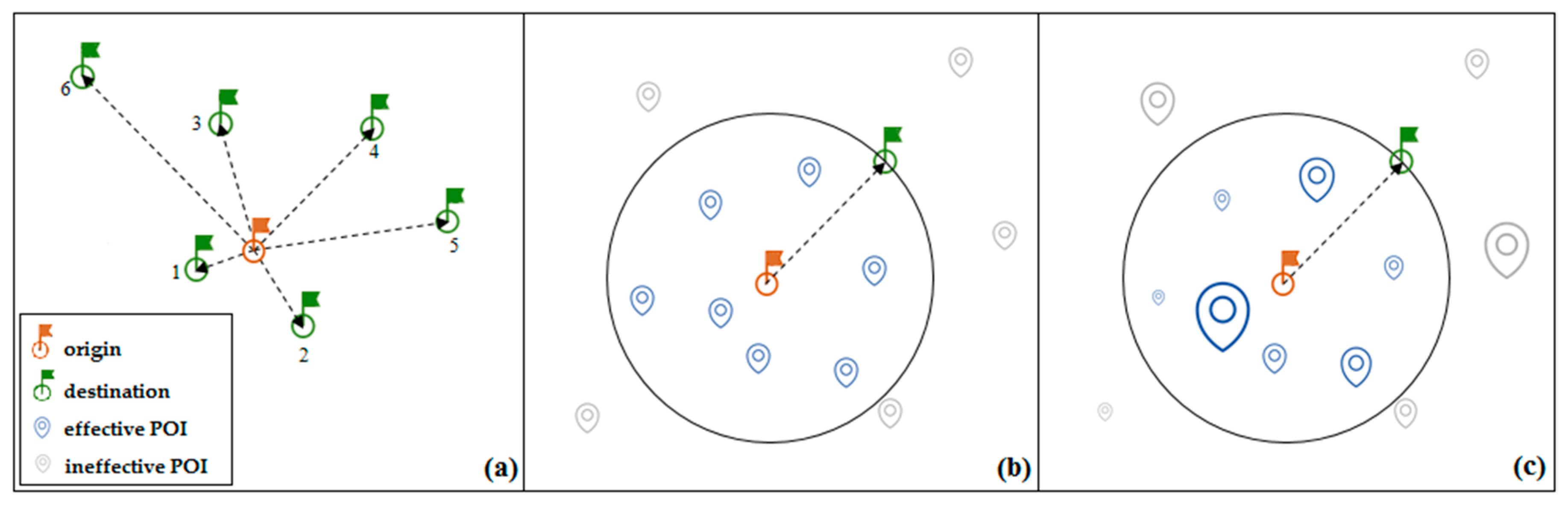
• First, we implemented the model using the common method of rank computation (i.e., computing the rank as rank-distance). This is more or less similar to the assumptions made in the gravity model. In this approach, the resultant distribution is not subject to change, because the distances between regions are constant. Figure 1a represents the schematic illustration of this scenario.
• Second, we employed the number of venues located in a circle centered at the origin with a radius equal to the distance between the origin and destination to compute the ranks. This way of computing the ranks is similar to that of an intervening opportunities model. With such an approach, resulting patterns are more dynamic. This is because new venues are created, some venues may shut down, or may be transferred to other regions. This scenario can be seen in Figure 1b.
• The third approach is to use check-in data for weighting the venues. Thus, humans have participated in the modeling, because venues are not the same in terms of mobility. For instance, cinemas attract much more people, in a certain period of time, than hotels. Therefore, since the amount of importance of venues, in terms of mobility are not the same, the relative importance should be taken into account. Therefore, we weighted each venue using check-ins occurred at that venue, so that more dynamicity can be reflected in the resultant patterns. The schematic view of this scenario is shown in Figure 1c.

Since the rank-based model is parameterized, a calibration procedure is needed to determine the adjustable parameter. This parameter serves, for geographers and planners, as a context and explanatory power in the model, so that different conditions of a study area can be taken into account. In this paper, due to its higher efficiency and simple implementation, the method introduced by Hyman was employed to determine the parameter [26]. The Hyman method tries to minimize the difference between the real average travel distance and modeled average travel distance in a repetitive manner [27]. In fact, the following equation should be minimized.

$$\mathrm{E}\left(\mathsf{\gamma }\right)=\left|\overline{\mathrm{r}}\left(\mathsf{\gamma }\right)-\overline{\mathrm{r}}\right|=\left|\frac{{{\displaystyle \sum }}_{\mathrm{i}}{{\displaystyle \sum }}_{\mathrm{j}}{\mathrm{T}}_{\mathrm{i}\mathrm{j}}\left(\mathsf{\gamma }\right){\mathrm{r}}_{\mathrm{i}\mathrm{j}}}{{{\displaystyle \sum }}_{\mathrm{i}}{{\displaystyle \sum }}_{\mathrm{j}}{\mathrm{T}}_{\mathrm{i}\mathrm{j}}\left(\mathsf{\gamma }\right)}-\frac{{{\displaystyle \sum }}_{\mathrm{i}}{{\displaystyle \sum }}_{\mathrm{j}}{\mathrm{T}}_{\mathrm{i}\mathrm{j}}{\mathrm{r}}_{\mathrm{i}\mathrm{j}}}{{{\displaystyle \sum }}_{\mathrm{i}}{{\displaystyle \sum }}_{\mathrm{j}}{\mathrm{T}}_{\mathrm{i}\mathrm{j}}}\right|$$

(5)

where $\overline{\mathrm{r}}$ is the average distance of observed trips and $\overline{\mathrm{r}}\left(\mathsf{\gamma }\right)$ is the average distance of predicted trips using the parameter $\mathrm{\gamma }$. Since obtaining a closed-form solution for Equation (5) is not straighforward, it should be minimized in a repititive manner. One way of solving the above equation is to use the Secant method. Algorithm 1 provides the pseudocode of the Secant method for solving the above equation.

Algorithm 1 Hyman method: pseudocode

1: Let ${\mathsf{\gamma }}_0$ (the initial value of the parameter) equal to $1/\overline{\mathrm{r}}$.

2: Compute the trip distribution matrix using ${\mathsf{\gamma }}_0$.

3: Calculate the average distance of predicted trips.

4: Consider the next approximation for the parameter as ${\mathsf{\gamma }}_1={\mathsf{\gamma }}_0\overline{\mathrm{r}}\left({\mathsf{\gamma }}_0\right)/\overline{\mathrm{r}}$.

5: while $true$ do:

6: Compute the trip distribution matrix using ${\gamma }_i$.

7: Calculate the average distance of predicted trips.

8: if $\left|\overline{\hat{\mathrm{r}}}\left({\mathsf{\gamma }}_{\mathrm{i}}\right)-\overline{\mathrm{r}}\right|<\mathsf{\epsilon }$ :

9: break while loop

10: else:

11: ${\mathsf{\gamma }}_{\mathrm{i}+1}=\frac{\left(\overline{\mathrm{r}}-\overline{\mathrm{r}}\left({\mathsf{\gamma }}_{\mathrm{i}-1}\right)\right){\mathsf{\beta }}_{\mathrm{i}}-\left(\overline{\mathrm{r}}-\overline{\mathrm{r}}\left({\mathsf{\gamma }}_{\mathrm{i}}\right)\right){\mathsf{\gamma }}_{\mathrm{i}-1}}{\overline{\mathrm{r}}\left({\mathsf{\gamma }}_{\mathrm{i}}\right)-\overline{\mathrm{r}}\left({\mathsf{\gamma }}_{\mathrm{i}-1}\right)}$

12: end if

13: end while

In addition, since the rank-based model presented in Equation (4) does not guarantee the equality of the real and predicted number of attracted trips, a balancing procedure called Furness is applied on the matrix. Algorithm 2 shows the pseudocode of the Furness algorithm that aims at minimizing the difference between the total number of real and predicted trips.

Algorithm 2 Furness method: pseudocode

1: Compute the trip distribution matrix.

2: Let ${\mathrm{T}}_{\mathrm{i}}^{\text{'}}$ and ${\mathrm{T}}_{\mathrm{j}}^{\text{'}}$ be sum of elements in row i and column j, respectively.

3: while $\left|{\mathrm{T}}_{\mathrm{i}}-{\mathrm{T}}_{\mathrm{i}}^{\text{'}}\right|>\mathsf{\epsilon }$ and $\left|{\mathrm{T}}_{\mathrm{j}}-{\mathrm{T}}_{\mathrm{j}}^{\text{'}}\right|>\mathsf{\epsilon }$ do:

4: Multiply each column by ${\mathrm{N}}_{\mathrm{j}}={\mathrm{T}}_{\mathrm{j}}/{\mathrm{T}}_{\mathrm{j}}^{\text{'}}$.

5: if $\left|{\mathrm{T}}_{\mathrm{j}}-{\mathrm{T}}_{\mathrm{j}}^{\text{'}}\right|<\mathsf{\epsilon }$ and $\left|{\mathrm{T}}_{\mathrm{i}}-{\mathrm{T}}_{\mathrm{i}}^{\text{'}}\right|<\mathsf{\epsilon }$:

6: break while loop

7: end if

8: Multiply each row by ${\mathrm{N}}_{\mathrm{i}}={\mathrm{T}}_{\mathrm{i}}/{\mathrm{T}}_{\mathrm{i}}^{\text{'}}$.

9: if $\left|{\mathrm{T}}_{\mathrm{j}}-{\mathrm{T}}_{\mathrm{j}}^{\text{'}}\right|<\mathsf{\epsilon }$ and $\left|{\mathrm{T}}_{\mathrm{i}}-{\mathrm{T}}_{\mathrm{i}}^{\text{'}}\right|<\mathsf{\epsilon }$:

10: break while loop

11: end if

12: end while

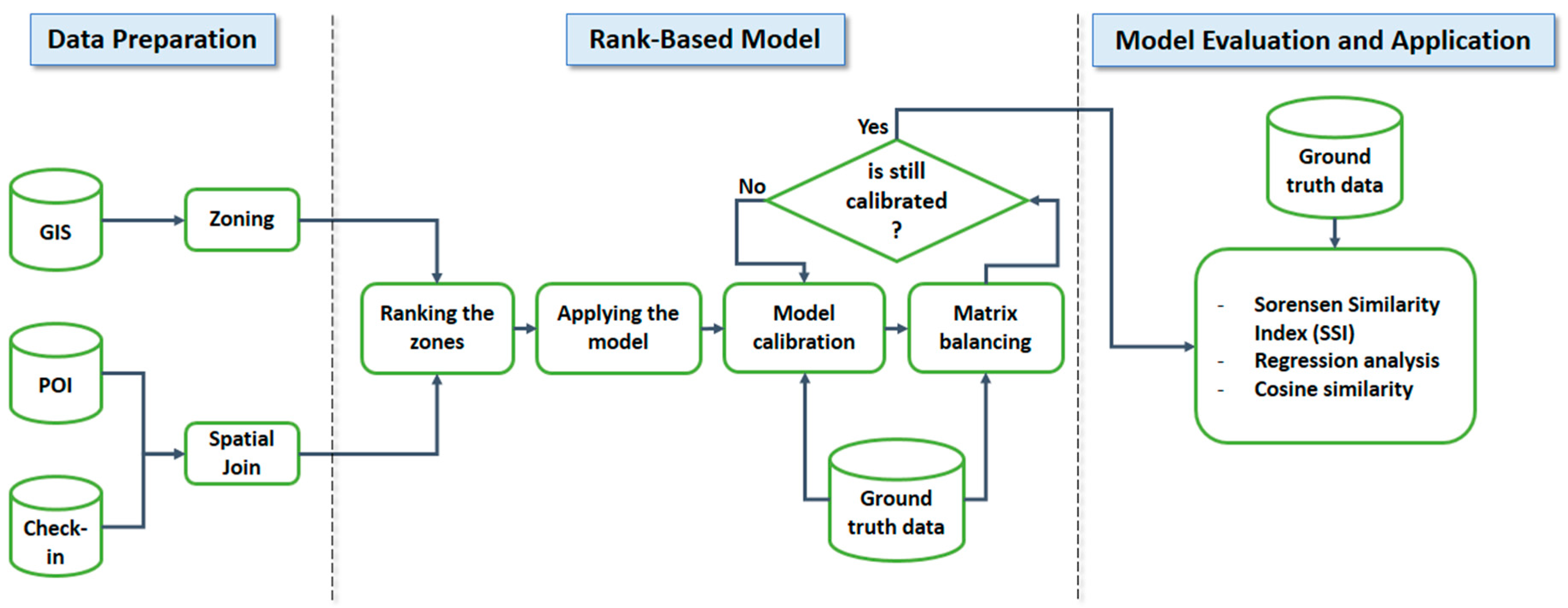
Figure 2 illustrates the steps required to apply the model. First, it is required for the study area to be partitioned into smaller parts, called zones. In addition, in order to compute the proposed ranking schema, information about location of venues and check-ins are required. Using these information, the zones are ranked. Then, the raw trip distribution matrix is obtained according to Equation (4). To find the best value of the adjustable parameter, the Hyman method is applied on the matrix. Also, the Furness method is applied on the matrix to balance it. Finally, the model is evaluated based on various criteria. If the results of evaluation are acceptable, the model along with the determined parameter can be employed to compute the distribution of mobility flow within the study area.

3. Study Area and Datasets Used

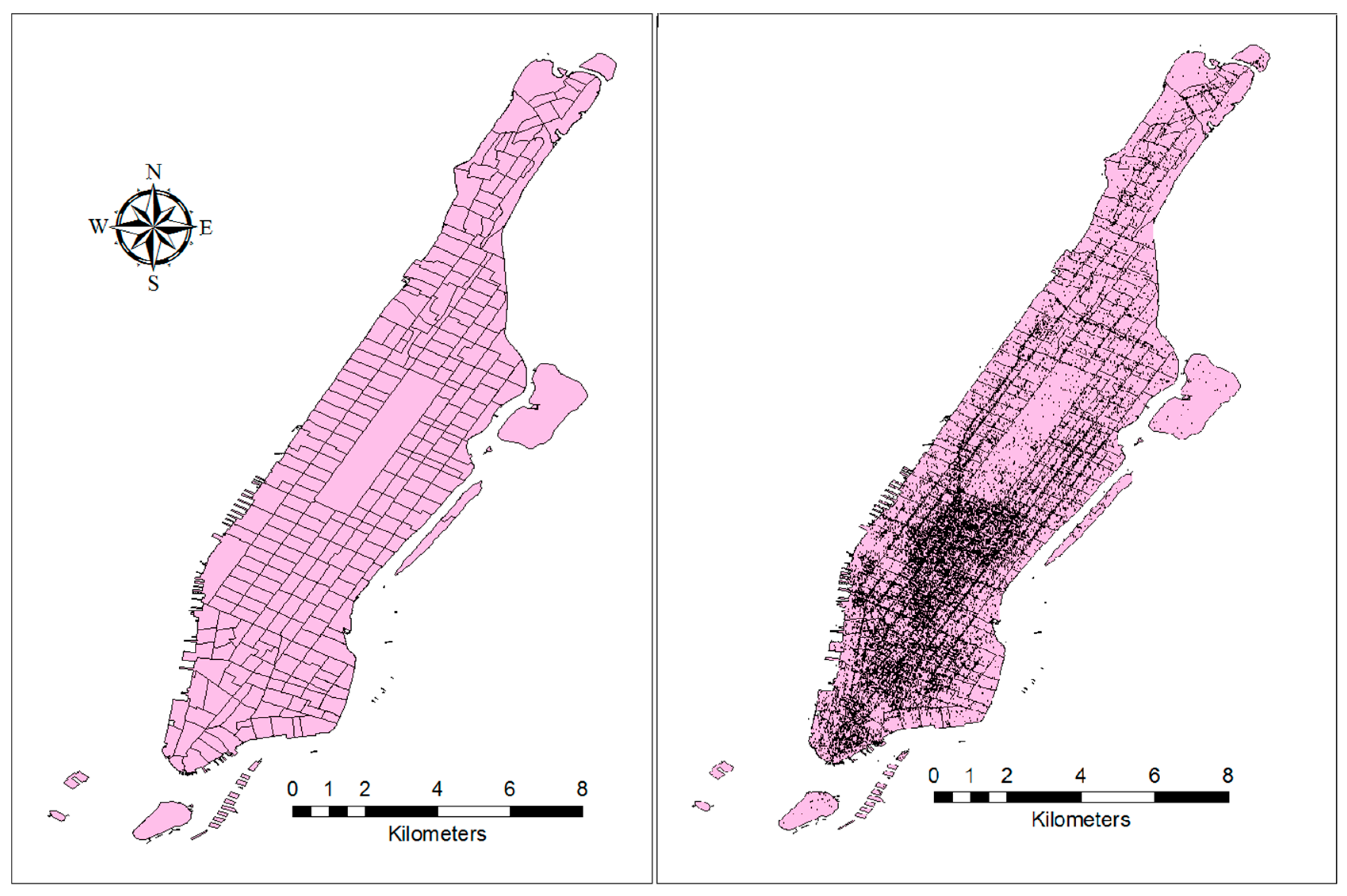
In this paper, we considered a census tract reference map of Manhattan as trip production and attraction zones. Manhattan is one of the most densely populated areas in the United States and the rate of mobility is, then, very high. Being one of the world’s major commercial and financial centers, Manhattan encounters a significant number of daily travels toward itself. In addition, thanks to the networks of tunnels, bridges, railroad lines, and subways that link Manhattan to the surroundings, there is an enormous influx of daily commuters from neighboring boroughs, including The Bronx, Brooklyn, Queens, and Staten Island, and even from New Jersey, Connecticut, and NYC suburbs such as White Plains and Long Island who are surely making various trips within Manhattan throughout the day [28]. Thus, modeling the mobility pattern within intra-urban areas such as Manhattan is among the challenges that the spatial interaction models are facing [8,29]. There are 288 zones in the 2010 census tract reference map of Manhattan. In addition to the GIS map of the study area, we used a dataset which includes long-term (about 18 months from April 2012 to September 2013) global-scale check-in data collected from Foursquare through its Twitter Application Programming Interface [30]. It contains about 33 million check-ins on about three million venues worldwide. The location of each venue within Manhattan was extracted from this dataset and mapped on the reference map. The distribution of venues over census tracts are shown in Figure 3.

In order to evaluate the results obtained from models and to compare the rank concepts, GPS traces of taxi vehicles over Manhattan were used. The datasets were collected and provided to the New York City (NYC) Taxi and Limousine Commission (TLC) under the Taxicab and Livery Passenger Enhancement Programs (TPEP/LPEP) (refer to Taxi and Limousine Commission website at http://www.nyc.gov/tlc). The yellow and green taxi trip records include fields capturing pick-up and drop-off dates/times, pick-up and drop-off locations, trip distances, passenger counts, and some other information about payment and rate types. Although taxi data are not representative of the whole mobility within a city, they can present it to some extent [17]. Usually, finer resolution datasets such as taxi data suffer from having many zero-counts. In order to improve the completeness of evaluation data, we combined yellow and green taxi traces. Since taxis are allowed to pick up passengers from other boroughs of NYC, only trips originating from (and ending in) Manhattan were considered. 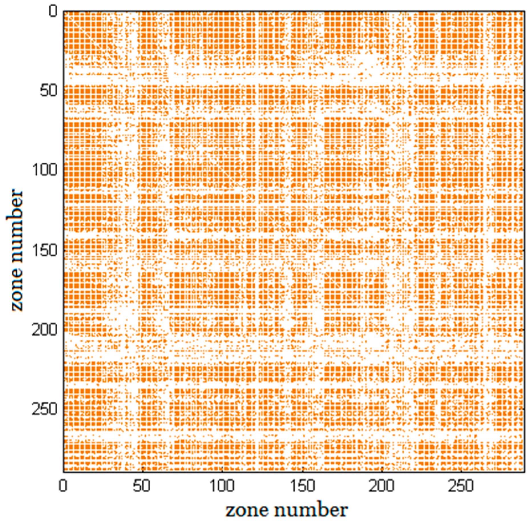Figure 4 visualizes the sparsity pattern of the ground truth matrix of the trip distribution.

4. Results and Discussion

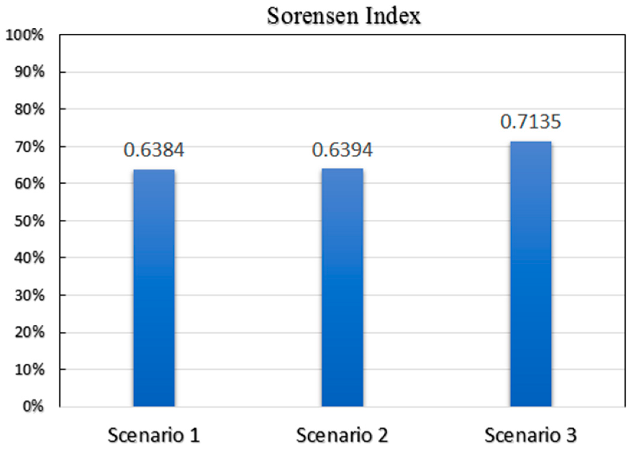
Following the research conducted by [31], the Sorensen Similarity Index (SSI), also known as Sorensen-Dice Index, was used as a measure of similarity between real and predicted trip distribution matrices. This index ranges from 0 to 1, where numbers closer to one indicate more similarity between two matrices. Figure 5 presents a comparison among the performances of different rank concepts in the model based on SSI. The Sorensen Similarity Index is shown in the following equation:

$$\mathrm{SSI}=\frac{2{{\displaystyle \sum }}_{\mathrm{i}}^{\mathrm{N}}{{\displaystyle \sum }}_{\mathrm{j}}^{\mathrm{N}}\min \left({\mathrm{T}}_{\mathrm{ij}},{\mathrm{T}}_{\mathrm{ij}}^{\prime }\right)}{{{\displaystyle \sum }}_{\mathrm{i}}^{\mathrm{N}}{{\displaystyle \sum }}_{\mathrm{j}}^{\mathrm{N}}{\mathrm{T}}_{\mathrm{ij}}+{{\displaystyle \sum }}_{\mathrm{i}}^{\mathrm{N}}{{\displaystyle \sum }}_{\mathrm{j}}^{\mathrm{N}}{\mathrm{T}}_{\mathrm{ij}}^{\prime }}$$

(6)

where ${\mathrm{T}}_{\mathrm{ij}}$ and ${\mathrm{T}}_{\mathrm{ij}}^{\text{'}}$ are ith and jth element of real and predicted trip distribution matrices and N is the total number of zones in the study area.

Figure 5 indicates that employing opportunities (venues) rather than distance in the rank-based model is not effective. However, according to the SSI, a check-in-weighted ranking schema will result in predictions that are more similar to reality.

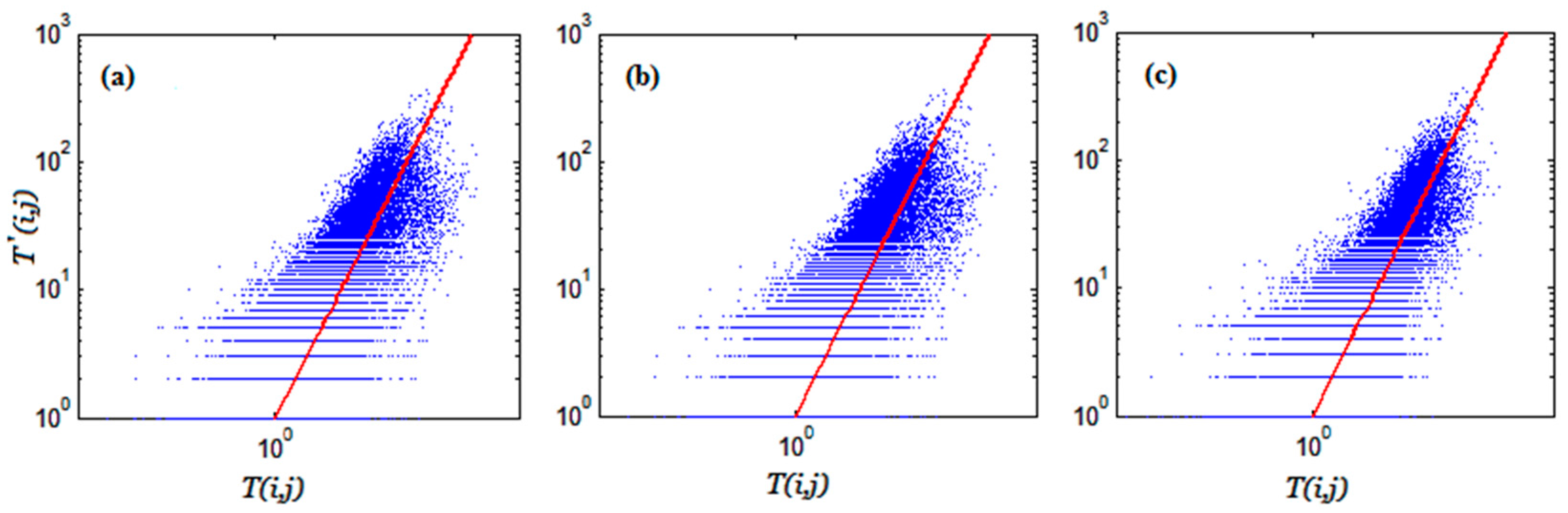
The scatter plot of predicted trips against observed trips for each scenario is shown in Figure 6. This plot shows the relationship between two matrices. The points in the plot correspond to individual elements of trip distribution matrices. The values on the vertical and horizontal axes are from real and predicted trip distribution matrices, respectively, and the plot is on a logarithmic scale. The red line is the identity line (y = x) where predicted number of trips are equal to the real number of trips. Obviously, the more the two matrices agree, the more the scatters tend to concentrate in the vicinity of the identity line.

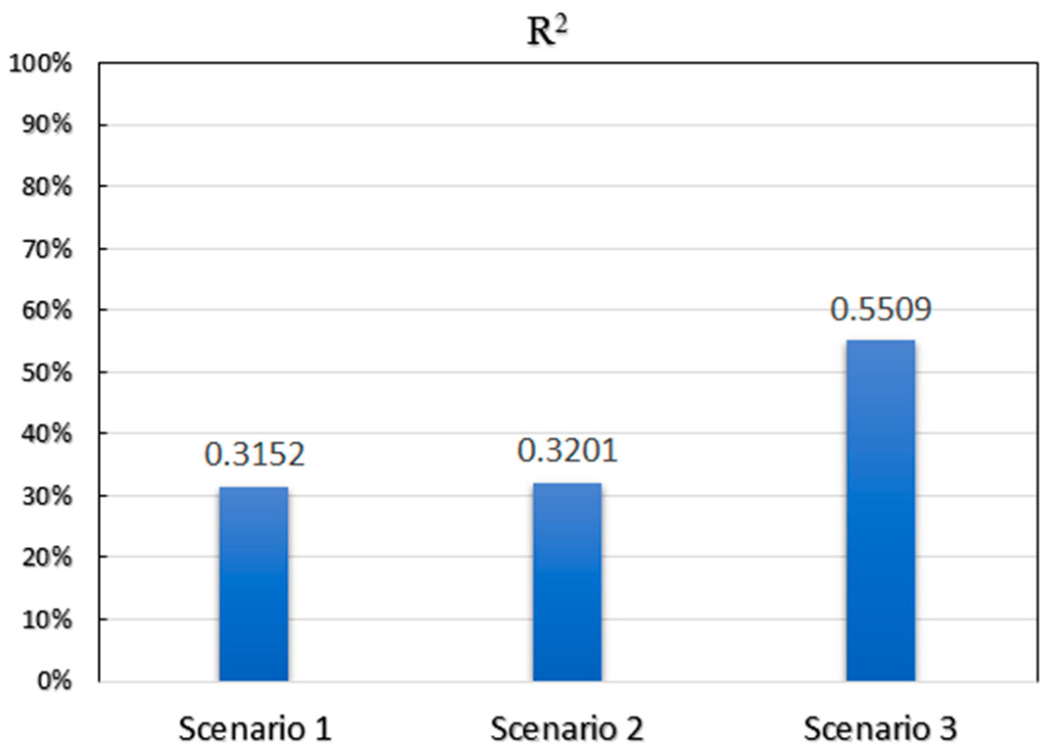
As can be seen from the above results, the difference between the two first scenarios is quite negligible. However, the scatter on the left is much narrower than the others and concentrated about the red line. To have a quantitative measure of how close the predicted numbers of trips are to the ground truth data, we determined R² values from the regression analysis applied on scatter plots of Figure 6. Figure 7 compares the results in terms of R².

Again, the difference between using rank-distance and number of venues is not remarkable. However, as Figure 7 illustrates, the value of R² for the model, along with a check-in-weighted rank concept, that has been dramatically increased.

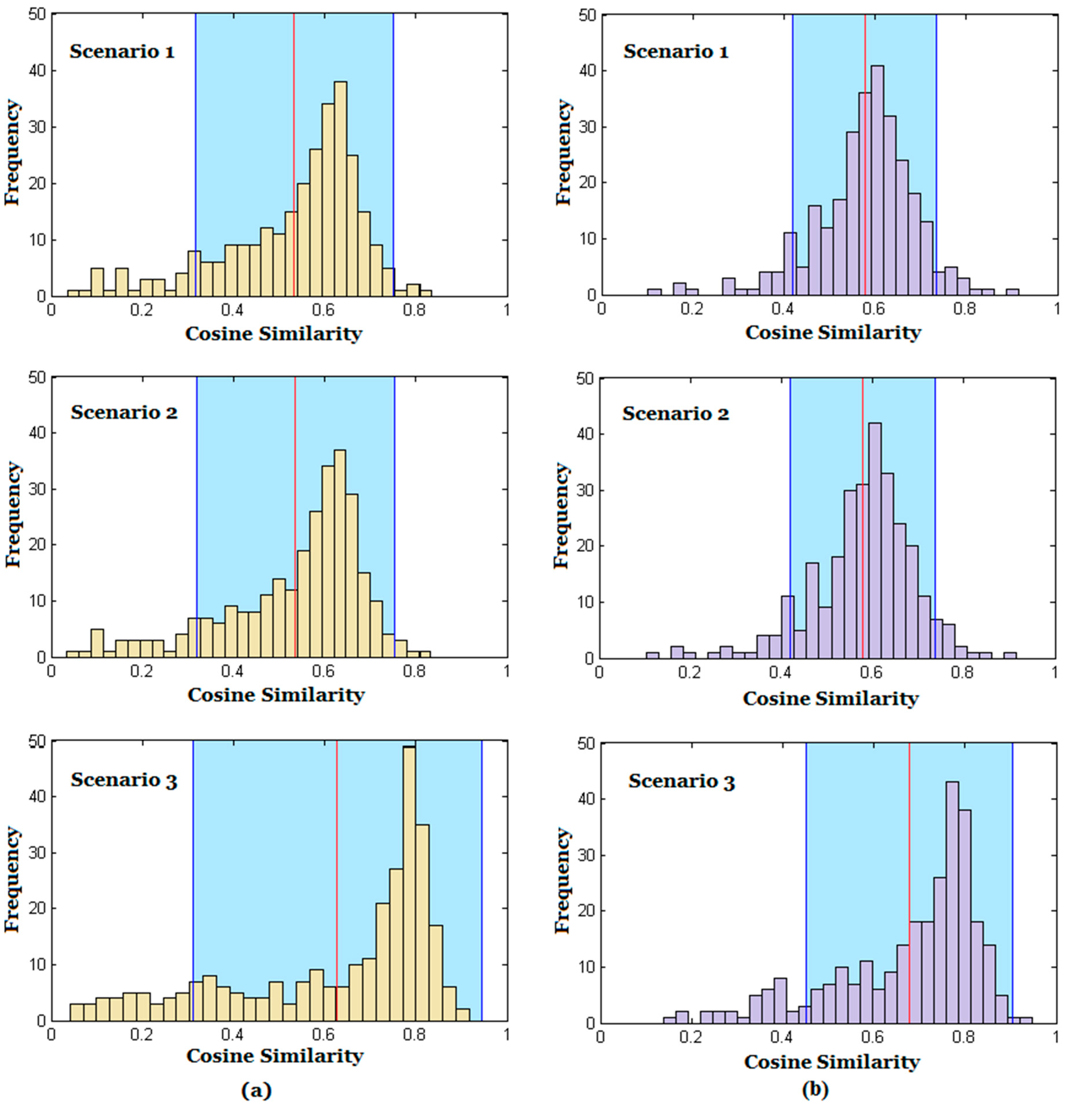
In order to analyze the results in a more detailed manner, we computed the cosine similarity between matrices at the zone level, rather than the city level. In fact, we partitioned the matrices row- and column-wise. Then, the cosine similarities between corresponding rows and columns were computed. In other words, each row (column) is considered to be a vector in a 288-dimensional space (i.e., the dimension of space is equal to the number of zones). Now, if the angle between this vector and the corresponding vector of the ground truth matrix in the space is equal to 0°, there will be a complete (1) similarity. On the other hand, if two vectors are in opposite orientations, the value of index will be −1. Since the trip distribution matrix is a non-negative matrix, the index practically ranges from 0 to 1, where 0 and 1 refer to perpendicular and parallel vectors, respectively. Figure 8 shows the frequency histograms of cosine similarities for rows and columns.

The red line refers to the mean value of the histogram ($\mu$) and the blue bounds show the interval $\mu -\sqrt{2}\sigma$ and $\mu +\sqrt{2}\sigma$, where $\sigma$ is the standard deviation. According to Chebyshev’s inequality, at least 50 percent of values lie within the blue area. The mean value of the histogram in the case of Scenario 3 is, again, higher than that of the others. In addition, the blue area has been forwarded toward higher similarities.

The reason for obtaining similar results for the two first scenarios can be attributed to the fact that as the radius of the circle between origin and destination is increased, the number of venues within this circle is also increased. As the rank-based model does not take into consideration the magnitude of differences between ranks, the resultant trip distributions will be similar for similar rank distributions. For example, in scenario 2, the number of venues located within each circle is counted. Then, these values are sorted out in a matrix and ranks are assigned to each element of the matrix. Clearly, the differences between ranks are always constant and equal to 1. However, the differences between the numbers of venues in the circles vary remarkably. This is a major disadvantage of the model. Although applying a weighting schema on the venues using check-ins changes the distribution of ranks within the matrix.

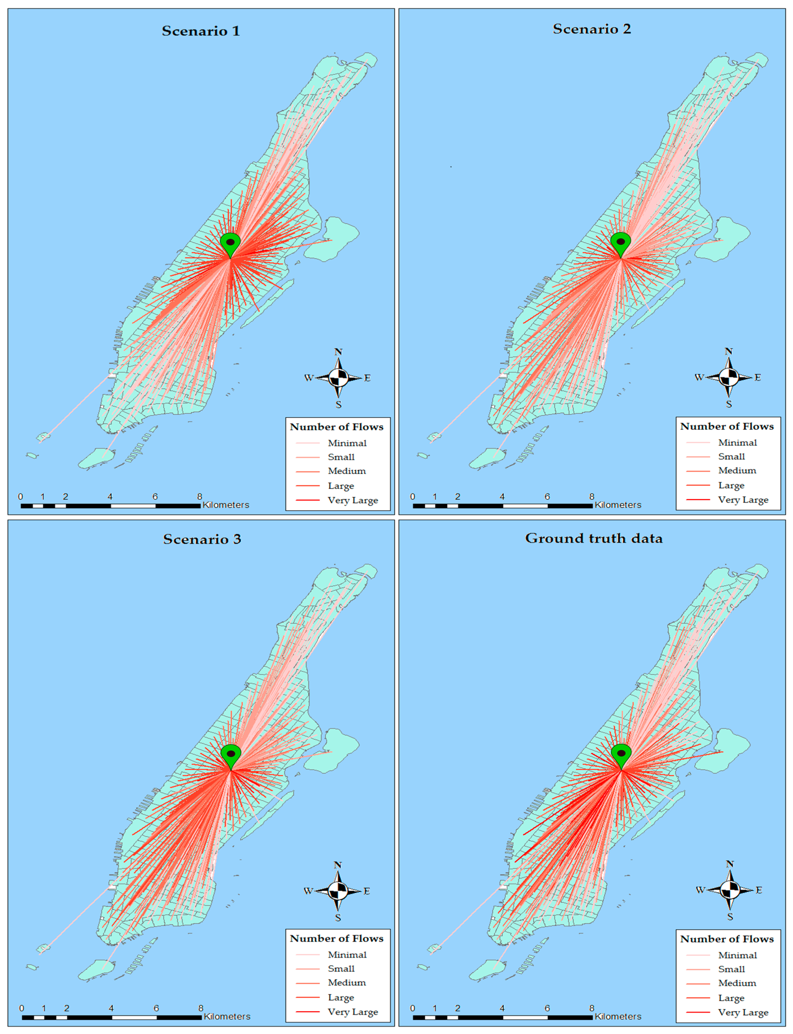
Figure 9 shows flow maps illustrating the interactions between Central Park of Manhattan, designated by a green pin, and other zones. Apparent in the upper maps is the fact that the trips in the two first scenarios are regularly distributed. However, the ground truth map indicates irregularities in the distribution which are too complicated to be modeled using a mere physical parameter such as distance. In fact, large flows, in these scenarios, are directed towards closer zones; while the lower left map conducts trips towards southern zones at which commercial and activity centers are located.

5. Conclusions

In this paper, we conducted research to study the concept of ranking, in a model of predicting collective human mobility, called a rank-based model. For this purpose, we proposed three scenarios including rank-distance, the number of venues in the region, and a check-in weighted venue schema to compute the ranks in the model.

Results show that the two first scenarios will result in very similar patterns. The reason is that as the distance between origin and destination increases, the number of venues located between them also increases. However, results of applying the third scenario show a remarkable increase in the accuracy of predictions. Therefore, check-ins play a significant role in improving the predictability of mobility patterns.

Considering the rank as distance and number of places of interest (POIs) is, to some extent, objective in the sense that they do not represent real specific conditions of a city. In other words, the concepts of distance and number of POIs are the same for all cities in the world. However, using check-in weights, has some aspects of reality added to the model. Surely, the role of a crowded park in human mobility is not the same as of a hotel, for instance. Thus, applying check-ins occurred at each POI will result in closer predictions to reality.

Moreover, using a check-in weighting schema, the dynamicity of human mobility could be accounted for. As check-in data are dynamic, they can consider the variations in people’s interests and behaviors. By using check-ins, any change in land use of POIs is also accountable. In addition, since ongoing events are reflected in check-in data, but not in distance and number of venues in the city, check-in data are particularly useful when events are in progress in the region. The use of check-in data to weigh the POIs implies no particular assumption or restriction on the study area. Since the assumptions made about the ranking method are independent of the study area and its conditions, the conclusions can be potentially generalized to any city. Although employing check-in data in the rank-based model resulted in more promising predictions, the differences between rank numbers is still fixed, and should be addressed in future works. In addition, the temporal dimension of human mobility has not been discussed in this paper. The applicability of the proposed method in spatiotemporal analysis of human mobility can be elaborated on in the future.

In a complex system, such as human mobility, the interactions between its many constituent parts (i.e., people, venues, distances, etc.) determine the properties of the system’s behavior (i.e., urban environments). The study of the relationships between the venues, people, and distance deepens our understanding of the urban properties. The usability of these relationships in real world applications, however, needs an accurate model of human mobility prediction. This study betters our understanding of human mobility by including dynamic aspects of destination selection in the rank-based model. Moreover, the increase in the accuracy of the resulting patterns using the proposed method also increases the applicability of the model in real world applications.