A Comparison of Terrain Indices toward Their Ability in Assisting Surface Water Mapping from Sentinel-1 Data

Abstract

The Sentinel-1 mission provides frequent coverage of global land areas and is hence able to monitor surface water dynamics at a fine spatial resolution better than any other Synthetic Aperture Radar (SAR) mission before. However, SAR data acquired by Sentinel-1 also suffer from terrain effects when being used for mapping surface water, just as other SAR data do. Terrain indices derived from Digital Elevation Models (DEMs) are easy but effective approaches to reduce this kind of interference, considering the close relationship between surface water movement and topography. This study compares two popular terrain indices, namely the Multi-resolution Valley Bottom Flatness (MrVBF) and the Height Above Nearest Drainage (HAND), toward their performance on assisting surface water mapping using Sentinel-1 SAR data. Four study sites with different terrain characteristics were selected to cover a very wide range of topographic conditions. For two of these sites that are floodplain dominated, both normal and flooded scenarios were examined. MrVBF and HAND values for the whole study areas, as well as statistics of these values within water areas were compared. The sensitivity of applying different thresholds for MrVBF and HAND to mask out terrain effect was investigated by adopting quantity disagreement and allocation disagreement as the accuracy indicators. It was found that both indices help improve water mapping, reducing the total disagreement by as much as 1.6%. The HAND index performs slightly better in most of the study cases, with less sensitivity to thresholding. MrVBF classifies low-lying areas with more details, which sometimes makes it more effective in eliminating false water bodies in rugged terrain. It is therefore recommended to use HAND for large scale or global scale water mapping. However, for water detection in complex terrain areas, MrVBF also performs very well.

1. Introduction

Water contributes to all aspects of economic and social development. Water supply, sanitation, and a healthy environment form the basis of successful poverty reduction and shared-growth strategies, especially in developing countries [1]. The spatial distribution of surface water informs about an important part of freshwater resources on Earth. Surface water bodies are dynamic in nature as they shrink, expand, or change their appearance with time, owing to different natural and human-induced factors. Variations in water bodies have been known to have significant impacts on other natural resources and human assets, and further influence climate change [2]. Under extreme conditions, drastic changes of surface water could cause serious disasters such as floods and droughts—two life-threatening and financially expensive natural disasters [3]. Therefore, it is crucial to understand the extent of water bodies and master their dynamics over time.

Remote sensing provides an efficient way of monitoring surface water bodies. Ever since the first remote sensing satellite was launched, it has been used for water detection [4]. There are generally two types of remote sensors that are powerful for detecting water from space, namely optical sensors and microwave sensors. The optical sensors utilize the low reflectance of water bodies in near infrared channels to achieve delineation of water and land. The principle for water detection using microwave sensors is based on the low backscatter signal of water surfaces. Both types of sensors have their own advantages and disadvantages. The microwave sensors are able to penetrate cloud and some vegetation cover, due to their much longer wavelength. Therefore, they can work under all weather conditions and be effective in detecting water bodies beneath low vegetation.

Synthetic Aperture Radar (SAR) sensors have been widely applied in detecting and monitoring water bodies due to their suitable spatial resolution, as well as the ability to penetrate cloud and vegetation cover [5,6]. Until recently, SAR sensors had a relatively low temporal frequency (about 24–35 days for acquisitions in the same geometric configuration) [7], which hinders the intensive monitoring of surface water variation. The launch of the Sentinel-1A satellite in 2014 has improved temporal frequency of acquisitions (every 3–12 days in Europe), associated with a 20 m spatial resolution. The launch of the Sentinel-1B satellite in 2016 further improved the temporal frequency to 3–6 days. Sentinel-1 data can be freely downloaded by every user from the Scientific Data Hub of the European Space Agency (ESA).

Several methods for mapping surface water bodies from SAR imagery have been developed. Visual interpretation is always one reliable and simple approach [8] except that it can be time consuming and subjective. Other popular methods include active contour models [9], texture-based segmentations [10], and grey-level thresholding [11]. Among all these methods, grey-scale thresholding is still the most commonly used approach to detect water areas using SAR imagery [12], due to its efficiency and acceptable accuracy. All pixels with a backscatter value lower than a specific threshold in an intensity image are classified as water. This threshold can be optimized using the Otsu algorithm [13], or through careful manual adjustment.

Bearing in mind the multiple advantages, there are also disadvantages using SAR for surface water detection. A serious and inevitable one is the terrain effect, because SAR sensors acquire data in a side-looking geometry. Therefore, mountains and hills may block the transmission and reception of microwave pulses, and thus introduce shadows and blind areas on SAR images. This usually impacts the water detection algorithms, especially when using grey-scale thresholding method, because the blocked areas also have low backscatter just as water surfaces do [14].

Surface water has a close relationship with the topography because of its fluid characteristics. Terrain information is thus useful in assisting water detection. There are many studies that have employed Digital Elevation Models (DEMs), digital representations of ground surface topography or relief, in detecting water bodies from remote sensing imagery [15,16,17]. More and more DEM data sources are becoming accessible, including Shuttle Radar Topographic Mission (SRTM) DEM with up to 1 arc-second resolution and TanDEM-X with 12 m resolution. High quality global terrain datasets, such as Advanced Spaceborne Thermal Emission and Reflection Radiometer Global Digital Elevation Model (ASTER GDEM) with 30 m resolution, are now available, which promotes the application of DEMs in assisting mapping surface water globally [18]. However, in most of these studies, DEM data are generally used for identifying those lower areas where water is more likely to be presented, or for estimating water level. The elevation itself is not ideal for helping delineating terrain shadows from water bodies, because shadow areas could be located in low areas and water could be held in high places sometimes.

Many terrain indices [19,20,21,22] have been developed in order to build up a stronger connection between water presence and topography. Most of these terrain indices can generally be categorized into two groups, valley bottom based and drainage based. A classic and popular one in the first group is the Multi-resolution Valley Bottom Flatness (MrVBF) proposed by Gallant and Dowling [23]. It tries to identify valley bottoms using a slope classification constrained to convergent areas, which is more likely to be occupied by water than simply low places. It has been used as an important data layer for mapping water bodies from remote sensing imagery in many studies [24,25,26]. A representative index in the drainage based group is the Height Above Nearest Drainage (HAND) index, which was presented by Rennó et al. [27] and implemented by Nobre et al. [28]. This index also attracted a lot of attention and has been applied in many water detection studies [5,29,30,31].

This study aims to conduct a comprehensive comparison on MrVBF and HAND indices, especially on their ability to assist surface water mapping using Sentinel-1A dual-polarized SAR data. A number of study sites with different topographic features under different inundation scenarios will be selected to showcase this comparison. Through this study, we are trying to elaborate the appropriate usage of these indices for the purpose of better surface water mapping, especially with SAR data.

2. Materials and Methods

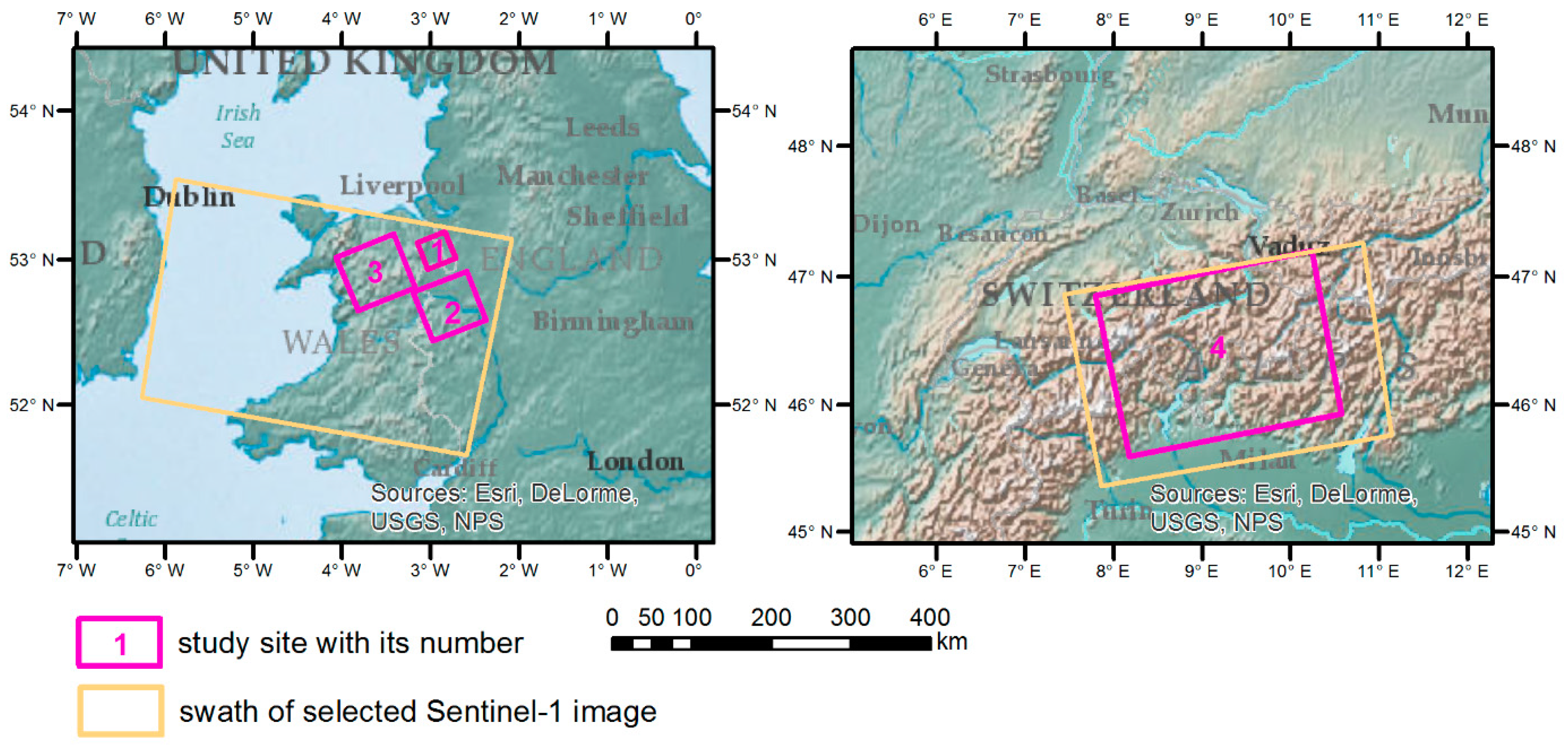
2.1. Study Sites

Rivers and lakes are two major types of surface water bodies. It is thus important that both types of water bodies are included in the study. Rivers that have experienced dramatic water change and lakes that are located in the mountainous areas are especially helpful for demonstrating the effect of terrain indices on water mapping. Therefore, four sites located in Europe were selected, as shown in Figure 1. Study sites 1, 2, and 3 are all in Wales, United Kingdom. Site 1 includes a section of River Dee which is on the upstream of Chester, as well as its floodplain area. Site 2 covers a section of River Severn at Shrewsbury along with its floodplain area. Both river sections experienced sharp flow dynamics in December of 2015. Site 3 is in the northwest part of Wales. It includes a part of Snowdonia National Park and Coed Y Brenin Forest Park with an average elevation over 350 m. This site has several main water bodies such as Lake Vyrnwy, Llyn Tegid, Llyn Trawsfynydd, Afon Tryweryn, Llyn Brenig, and Alwen Reservoir. Site 4 is to the north of Milan, covering a section of the border between Switzerland and Italy. It is a mountainous area with an average elevation over 1600 m. Main water bodies in this site include Lago Maggiore, Lago di Lugano, Lago di Como, and Brienzersee.

2.2. SAR Data

For study sites 3 and 4, where the water bodies are mainly lakes and ponds whose water extents are relatively stable within a short time period, only one image was selected for each site. For the floodplain dominated sites (1 and 2), images that captured a flood event were also selected. Hence, in total, six cases were analyzed in this study, as listed in

Table 1. Synthetic Aperture Radar (SAR) images selected for each study site.

Study Site	Code for Study Case	Data of Acquisition	Sensor Mode	Pass	Incident Angle	Resolution
1	Study site 1(A)	3 December 2015	Interferometric Wide Swath	Descending	33.258–35.266	5 × 20 m
	Study site 1(B)	27 December 2015
2	Study site 2(A)	3 December 2015	Interferometric Wide Swath	Descending	31.051–35.012	5 × 20 m
	Study site 2(B)	27 December 2015
3	Study site 3	27 December 2015	Interferometric Wide Swath	Descending	34.928–38.910	5 × 20 m
4	Study site 4	16 May 2015	Interferometric Wide Swath	Ascending	32.067–43.855	5 × 20 m

. River Dee in study site 1 experienced a flood event at the end of December 2015, thus its floodplain experienced a water expansion between 3 December 2015 and 27 December 2015. River Severn at Shrewsbury encountered a water level rise at the start of December, therefore, the floodplain site 2 had shrinking water bodies between these two dates. A code of (A) or (B) was given to each of these dates. Interferometric Wide (IW) Swath mode Sentinel-1 data for these study sites on the selected dates were downloaded from the ESA Scientific hub website (https://scihub.copernicus.eu/dhus/). Their swaths are displayed in Figure 1. These data are C-band dual-polarization (VV, VH) SAR data. They are standard Level-1 Ground-Range Detected High (GRDH) Resolution product generated from Level-0 data using the ScanSAR technique by ESA.

2.3. DEM Data

The most commonly used and freely available DEM is the SRTM DEM, which covers 85% of the Earth’s surface. In this study, both 3 arc-second (3s) and 1 arc-second (1s) spatial resolution SRTM DEMs were used. Two key properties of a DEM, the horizontal resolution and the vertical accuracy, are important in surface water mapping [32]. Vertical errors of the SRTM DEM are ±16 m and ±6 m for absolute and relative accuracy, respectively. The horizontal positional accuracy is ±20 m at a 90% confidence level [33]. Strozzi, et al. [34] compared the 1s SRTM DEM to an aero-photogrammetric DEM at a high-elevation mountain site in the Swiss Alps, and identified an average height difference of 7 m, a standard deviation of height difference of 36 m, and maximum errors of up to 285 m. Also using an aero-photogrammetric DEM as the reference, Kääb [35] found a standard deviation of the height difference of ±20 m, with maximum vertical deviations of −193 m and +143 m. Other studies in relatively flat terrain reported a Root Mean Square Error (RMSE) of SRTM DEM data of about 10 m in comparison with shuttle laser altimeter data [36]. Both 1s and 3s SRTM DEMs are stored in Integer type, which means the minimum elevation difference is 1 m.

3. Methodology

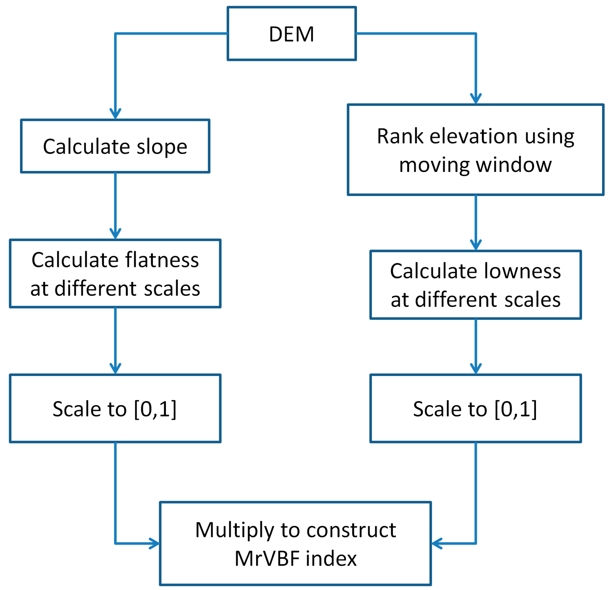
3.1. Calculation of MrVBF Index

The MrVBF index can be used for identifying valley bottoms at a range of sizes and slopes. It does not rely on a prior identification of channels and can depict unchanneled valley areas including perched swamps and lake wetlands [23]. It is an index that integrates the flatness and lowness characteristics of valley bottoms. Flatness is measured by the inverse of the terrain slope. Lowness is measured by a ranking of elevation with respect to a circular surrounding area. In order to identify different scales of valley bottoms, the flatness and lowness calculation are carried out through a series of scales. Both the measures of flatness and lowness were scaled to the range between 0 and 1, and then multiplied to construct the MrVBF index (Figure 2). MrVBF values range from 0 to a positive integer value. Increasing MrVBF values indicate a reduction in slope and broadening of the valley.

There are six key parameters in calculating MrVBF from DEM data, the initial threshold for slope (Ts), the lower and upper thresholds for elevation percentile (TeL, TeU, respectively), the shape parameter for slope and elevation percentile (Ss, Se, respectively), and the maximum resolution (Rm). The calculation of MrVBF has been implemented in SAGA-GIS, with an interactive interface for parameter input.

The MrVBF algorithm was originally developed using 1s resolution DEMs, but can be applied at any resolution, provided appropriate adjustments are made. The link between size and flatness of valley bottoms is incorporated into the algorithm by reducing the slope threshold by a factor of 2 at each step, and it is assumed that the relationship between slope threshold, resolution, and MrVBF value does not vary between landscapes or with DEMs of different resolutions. If the DEM resolution is substantially different from 1s, the initial slope threshold (Ts) must be adjusted to retain the relationship between slope and resolution. In this study, Ts for 1s DEM was set to be 16%, while that for 3s was set to be 8%, as suggested by Gallant and Dowling [23]. The other parameters used the same default values.

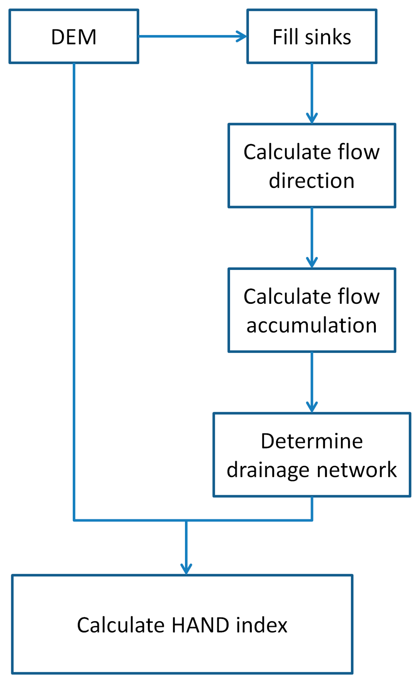
3.2. Calculation of HAND Index

The HAND index is generated using two sets of procedures. The first one is to condition the input DEM data, fixing sinks, defining flow paths, calculating an accumulated area map, and defining the drainage networks based on the accumulation map. The second procedure uses local drain directions and the drainage network to generate the nearest drainage map. Each pixel on this map is spatially associated with all DEM pixels draining into it. Then, each DEM pixel will have an elevation difference with its associated nearest drainage pixel. This elevation difference is assigned as the HAND index value for this DEM pixel, therefore, the unit of HAND value is meter.

The HAND model programme includes embedded routines for processing the DEM, filling sinks, and generating flow direction for each cell in the DEM using the so-called D8 approach [37], and routines for determining flow paths and the drainage network, as well as routines for calculating the height difference between each DEM pixel and its nearest drainage pixel, which is defined from the drainage network (Figure 3). This workflow has been implemented as Topography Tools in ArcGIS. These tools were employed in this study to generate HAND images from 1s and 3s SRTM DEMs.

Theoretically, the HAND value for drainage pixels is 0, and all the other pixels should have a HAND value great than 0, with a higher value indicating more unlikely to be held by water [27], while with a HAND value that is closer to 0, it is easier to be inundated by water. Inherited from the DEM data, the minimum difference of a HAND value is also 1 m.

3.3. Water Mapping

Selected Level-1 Sentinel-1 GRDH images were preprocessed and resampled into 10 m pixel spacing grid backscatter images using the SAR Geophysical Retrieval Toolbox (SGRT) [38] developed by Vienna University of Technology. SGRT is written in Python programming language and includes some external software modules, in particular ESA’s Sentinel-1 toolbox (S1TBX) for SAR data geocoding, radiometric corrections, and calibration. 3s SRTM data were employed for SAR terrain correction.

Reference water maps for each of the study cases were derived by manually thresholding both VV and VH backscatter data. Referring to a high-resolution Google Earth image, Sentinel-2, and Landsat images, some masking and digitalization work was also carefully conducted to improve the thresholding results. The final results were employed as the “actual” water maps for each study case.

4. Results and Discussion

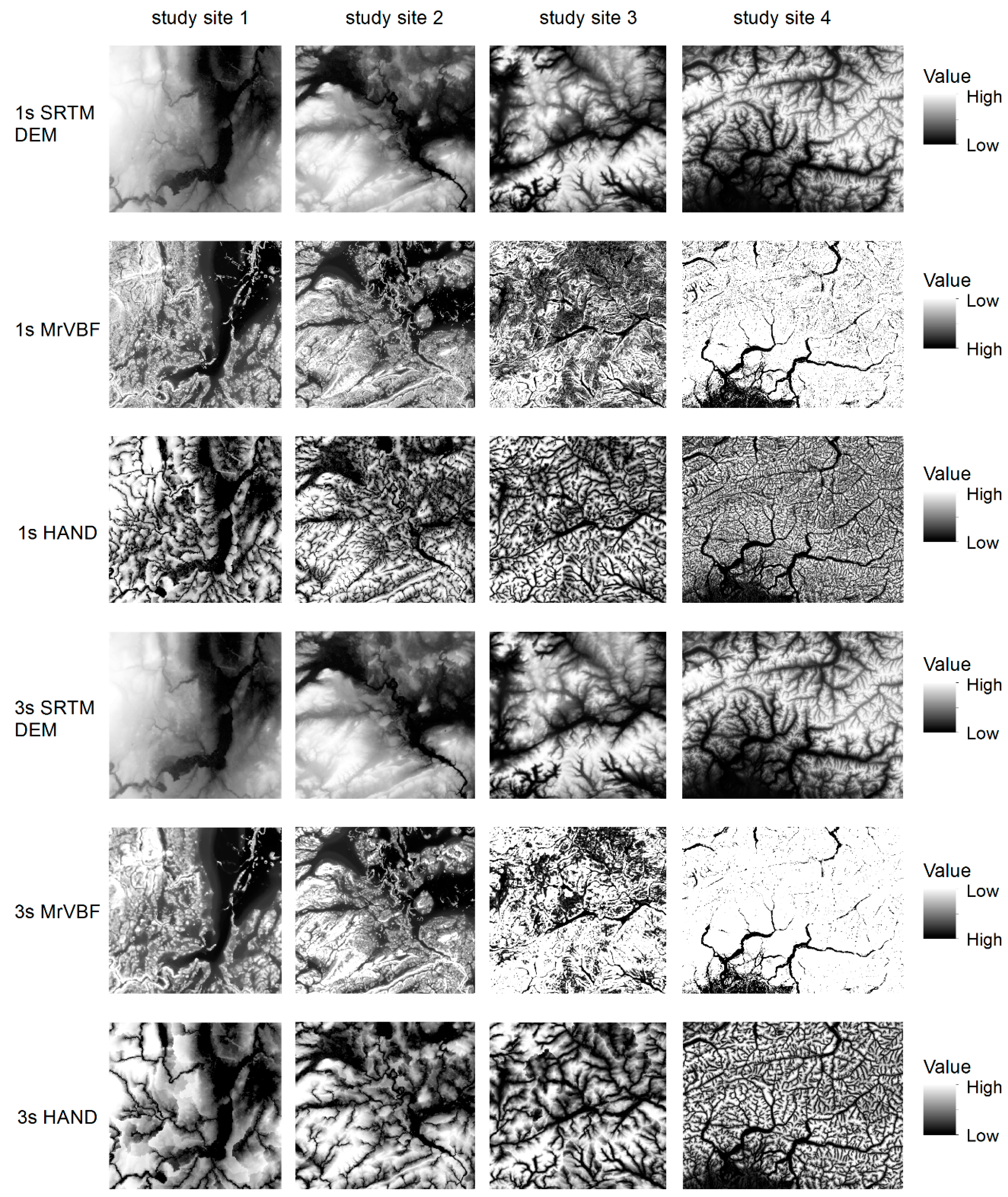
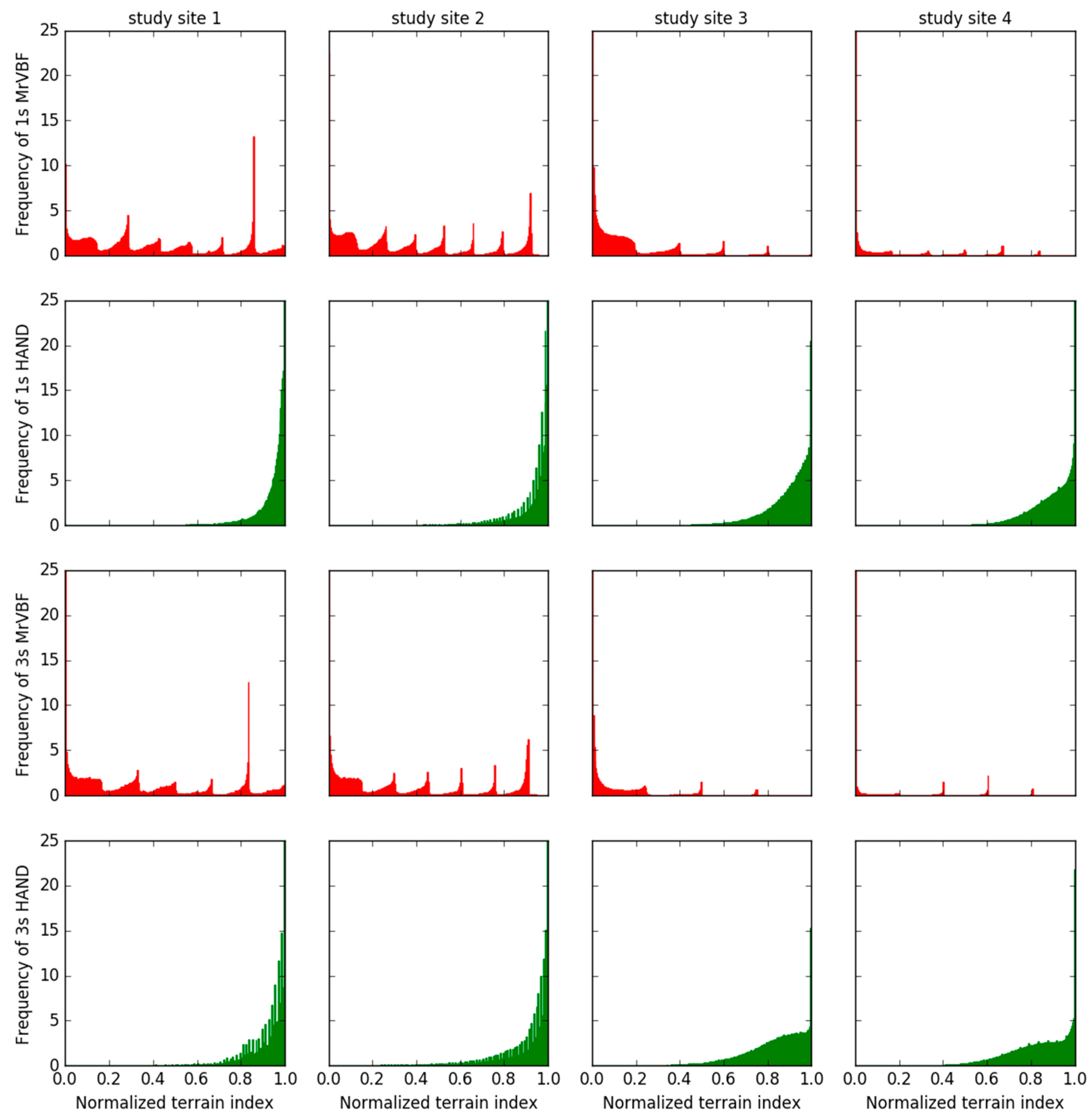
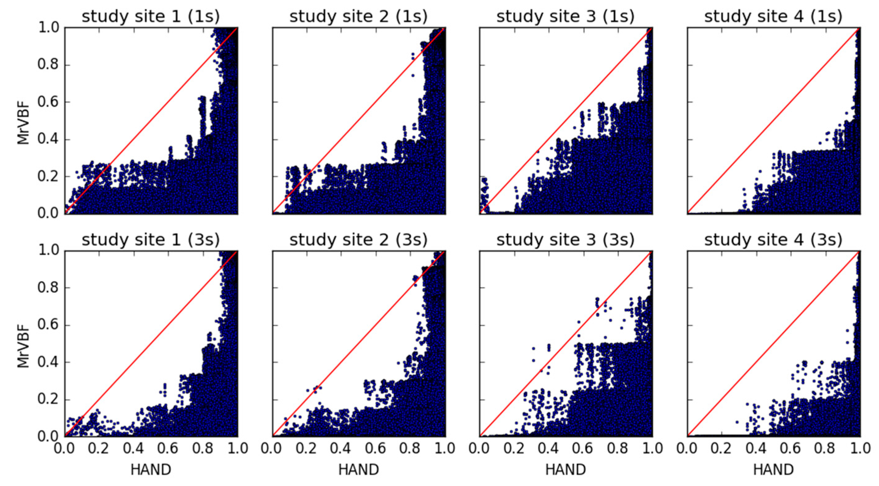
4.1. MrVBF Value vs. HAND Value

Both 1s and 3s SRTM DEM data of the selected four study sites were used to generate MrVBF and HAND images using the aforementioned approaches. They are all displayed in Figure 4. The original DEMs are also displayed for reference. All images are stretched using histogram equalization for a better visual effect. For the DEM images, darker color represents lower elevation. For MrVBF images, darker color stands for higher MrVBF value. For HAND images, darker color means lower HAND value. The values of these MrVBF images range from 0 to 7, with maximum values varying from different sites and resolutions. The maximum MrVBF value in a 3s image is generally lower than that in a 1s image for the same site, because the MrVBF values derived from 3s DEM in the first processing step correspond to those derived in the second step when using a base 1s resolution, according to Gallant and Dowling’s algorithm [23]. For the relatively flatter sites, the maximum MrVBF may be even higher than those of the mountainous areas (site 3 and 4). The HAND images keep more information from the original elevation. Values of HAND images range from 0 m to several hundred meters, depending on the original terrain of the study sites.

It can be seen from Figure 4 that all images show similar patterns for each site. Low-lying areas, which are dark in the DEM images, generally have high MrVBF values and low HAND values. HAND images keep more topographic patterns than MrVBF images. MrVBF images have higher contrast in mountainous sites (3 and 4) while lower contrast in others. For both indices, higher resolution images embrace more details and more complicated texture than their corresponding lower resolution images.

For a better comparison, both MrVBF and HAND indices were normalized to [0, 1] using the Min-Max Normalization. In particular, HAND index was normalized inversely with the maximum HAND value assigned a value of 0 and the minimum HAND value set to be 1. Then, normalized MrVBF and HAND indices would have similar meanings, which is higher value indicating higher possibility to be covered by water. Histograms of the normalized index images were generated and displayed in Figure 5. The maximum values of all y-axes (frequency) were set to be 25 for a better visualization of the histograms. It can be seen from Figure 5 that the distribution patterns of normalized MrVBF values and HAND values are quite different. The distribution of HAND values is more continuous than that of MrVBF values, with most of the pixels having values close to 1 (normalized value). The distributions of MrVBF values usually have several small peaks across the whole value range, with each peak representing the valley bottom pixels at one level of resolution. For sites 3 and 4, a large number of normalized MrVBF values are gathered near 0.

Scatterplots were produced to compare normalized MrVBF and HAND indices pixel-by-pixel (Figure 6). A red line representing the 1:1 relationship was drawn in each plot for reference. It can be seen from Figure 6 that normalized MrVBF is generally smaller than normalized HAND values; most of the scatter points occur under the 1:1 red line. In the up-right corner where scatter points represent pixels with the highest probability of water presence, HAND values are more concentrated to 1. This means that more pixels in the HAND image are able to acquire the highest water presence likelihood, while the MrVBF values of these pixels have a relatively higher variation.

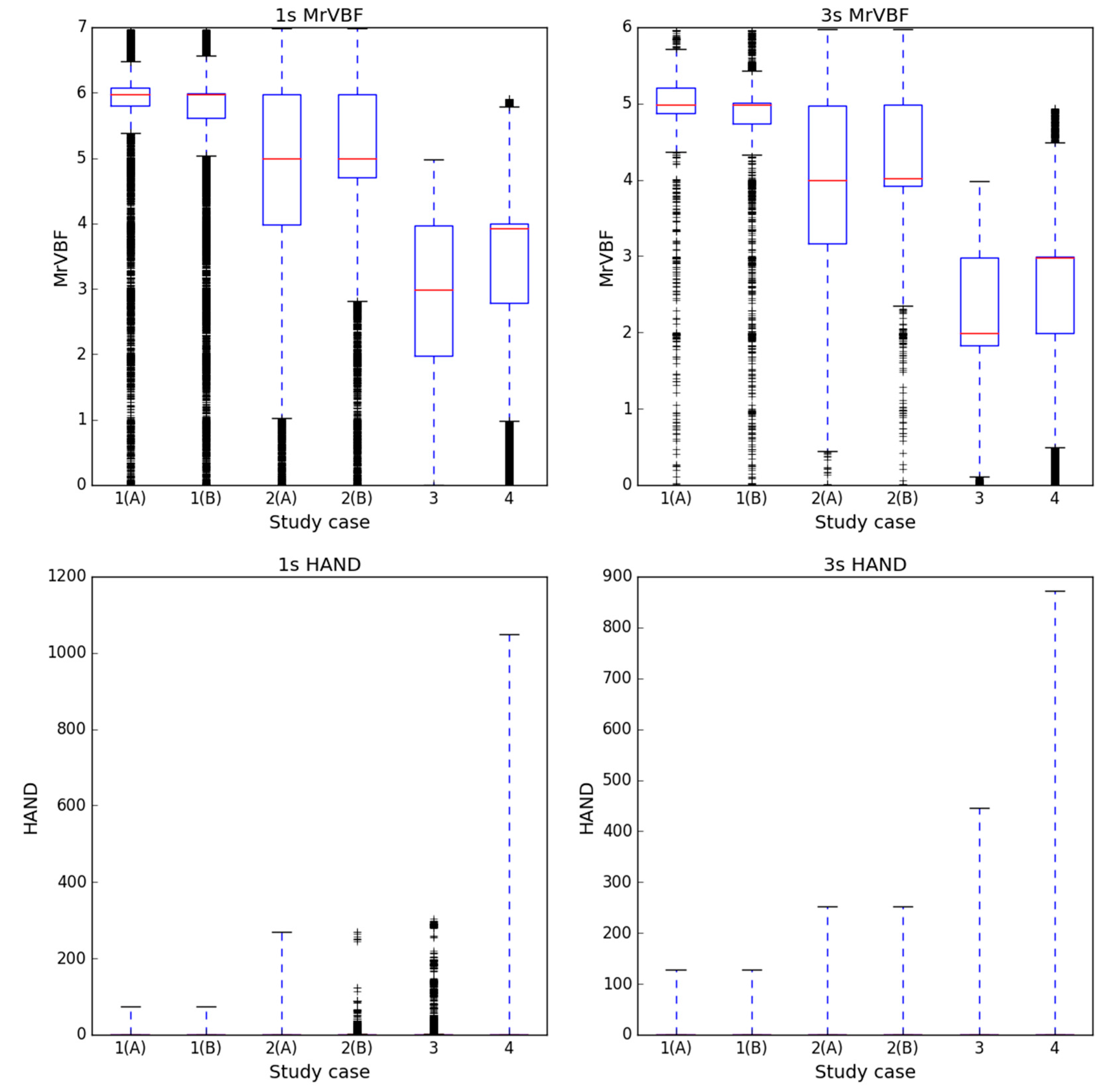
4.2. MrVBF Value vs. HAND Value within Water Areas

The actual water areas were used as masks for each study case to statistically analyze MrVBF and HAND values within them. Boxplots showing the minimum, first quartile (25%), median, third quartile (75%), and maximum values are displayed in Figure 7. Median values were shown as red lines inside the boxes. Outliers were also displayed, shown as black crosses. It is clear from Figure 7 that distribution patterns of different resolutions are similar, both for MrVBF and HAND. MrVBF values of both resolutions in water areas are distributed in the middle of the whole value range, varying from different sites, though the median values of 3s MrVBF are generally smaller than those of 1s MrVBF. In relatively flatter study sites, such as site 1 and 2, the median values as well as the whole box are higher. Most of the HAND values in water areas are 0, which is why the box parts below the third quartile are all overlapped with the horizontal axis. Maximum HAND values differ from sites. They are generally higher in mountainous sites than in flatter floodplain sites.

We also calculated the standard deviations (SDs) of both MrVBF and HAND values within water areas of each study case and listed them in

Table 2. Standard deviations (SDs) of MrVBF and HAND values within water areas.

Study Site	Code for Study Case	SD of 1s MrVBF	SD of 1s HAND	SD of 3s MrVBF	SD of 3s HAND
1	Study site 1(A)	1.301	2.754	1.043	11.669
	Study site 1(B)	1.300	2.061	1.095	7.782
2	Study site 2(A)	1.340	5.748	1.178	4.911
	Study site 2(B)	1.245	6.347	0.992	6.015
3	Study site 3	1.288	21.521	1.021	19.792
4	Study site 4	1.333	15.215	0.993	14.543

. They indicate the variations of terrain index values within water areas. It has to be noted that the SDs of MrVBF are not comparative to those of HAND, because they have different units. We can see from Table 2 that SDs of MrVBF in different cases are close, with relatively higher values in higher resolution. SDs of HAND in different cases have larger variations than those of MrVBF. Study sites 3 and 4 have relatively higher SDs than the others, meaning more fluctuations of HAND values within water areas in mountainous regions than in flatter regions.

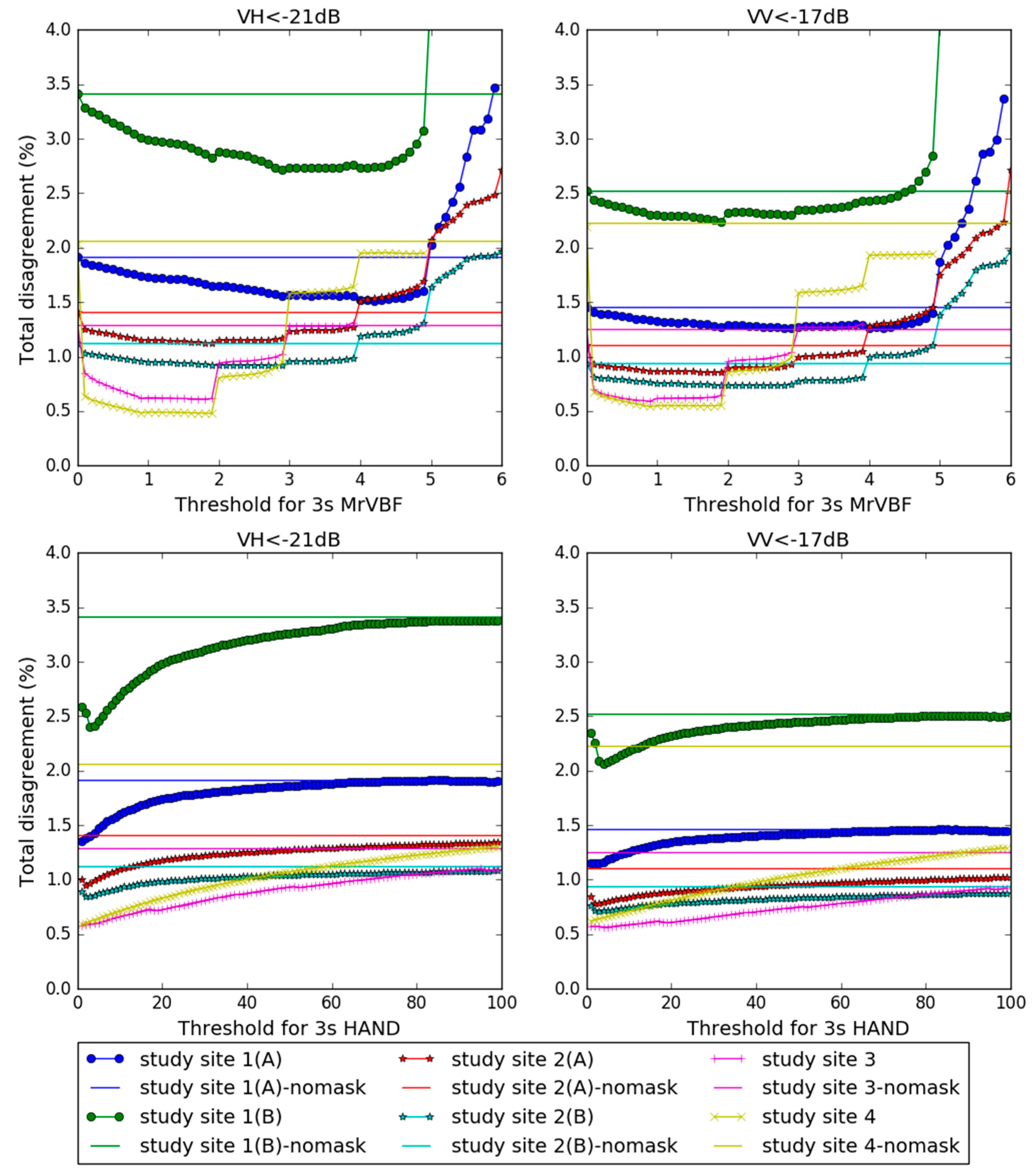
4.3. Sensitivity of MrVBF and HAND Thresholding

Through careful adjustment while comparing with the actual water maps, the threshold for delineating potential water was set to be −21 dB for VH or −17 dB for VV. These thresholds are able to ensure that water bodies in all the study cases were almost fully mapped. However, large commission errors in non-water areas are observed. The role of MrVBF and HAND index images is exactly to remove these errors as much as possible. For a MrVBF image, pixels with smaller values have lower probabilities of holding surface water, a lower limit thresholding on MrVBF is thus able to mask out some of the commission errors. While for a HAND image, pixels with higher values represent lower probabilities of water presence, an upper limit is then needed to threshold this image for reducing commission errors. Assuming a threshold (ζ or δ) was used for a MrVBF or a HAND image to assist surface water detection from a Sentinel-1 image here, the water areas would be derived based on one of the following criteria.

• (VH < −21 dB and MrVBF > ζ) or (VV < −17 dB and MrVBF > ζ);
• (VH < −21 dB and HAND < δ) or (VV < −17 dB and HAND < δ).

It is obvious that different threshold values generate different water maps. It is thus necessary to examine a series of thresholds to find the optimal one that helps deriving the best water map, in comparison to the referencing water body areas. There are several indicators that are commonly used to measure the accuracy of water mapping. Pontius and Millones [39] proposed a useful and simple approach for accuracy assessment that focuses on two components of disagreement between maps in terms of the quantity and spatial allocation of categories, namely quantity disagreement (Q) and allocation disagreement (A). Quantity disagreement is defined as ‘the amount of difference between the reference map and a comparison map that is due to a mismatch in the proportion of the categories’, whilst allocation disagreement is defined as ‘the amount of difference between the reference map and a comparison map that is due to less than the optimal match in the spatial allocation of the categories, given the proportions of the categories in the reference and comparison maps’, according to Pontius and Millones [39]. It was believed that this measurement is superior to Kappa coefficient because the value of both types of disagreements is more meaningful than a Kappa value whose baseline is randomness. Therefore, in this study, these two disagreements and their summary, total disagreement (TD), were employed as the indicator for accuracy, instead of the Kappa coefficient, which has been widely used for decades [39].

We examined ζ values from 0 to the maximum value for a MrVBF image with a step of 0.1, and plotted the corresponding TD in Figure 8. Considering HAND value greater than 100 stands for a very high place where water is usually impossible to be hold, we only examined δ values from 0 to 100 with a step of 1, in order to reduce unnecessary computation. TD derived from using different δ values on a HAND image were plotted in Figure 8 as well. The TD for each study case that was derived by simply thresholding on VV or VH image without a terrain mask is also displayed in Figure 8, shown as a constant horizontal line. Here, only those thresholding results of 3s images are displayed. Results for 1s DEM showed a similar pattern.

It is observed from Figure 8 that VV and VH perform similar in all of these study cases. When no terrain mask is applied, water bodies mapped merely from either VV or VH images have close accuracy. The biggest TD difference happens in study site 1(A), where TD thresholding on VH is about 3.4%, and on VV is about 2.5%. For the other study cases, the TD differences between VV thresholding and VH thresholding are all less than 0.5%.

Almost all the choices of threshold values have a positive impact on surface water detection. Their corresponding disagreements are lower than that of non-masked results, except when the threshold for MrVBF is too high, the disagreement can be even higher than that of non-masked results. This is because some correct water bodies would be masked out with an unreasonably high threshold. While using HAND, as the threshold increases, the disagreement becomes closer to that of the non-masked result, suggesting a weaker masking effect. All study cases demonstrate that involving terrain indices, either MrVBF or HAND, improves the accuracy of water mapping. Total disagreement can be reduced by as much as 1.6%, varying from different sites and methods.

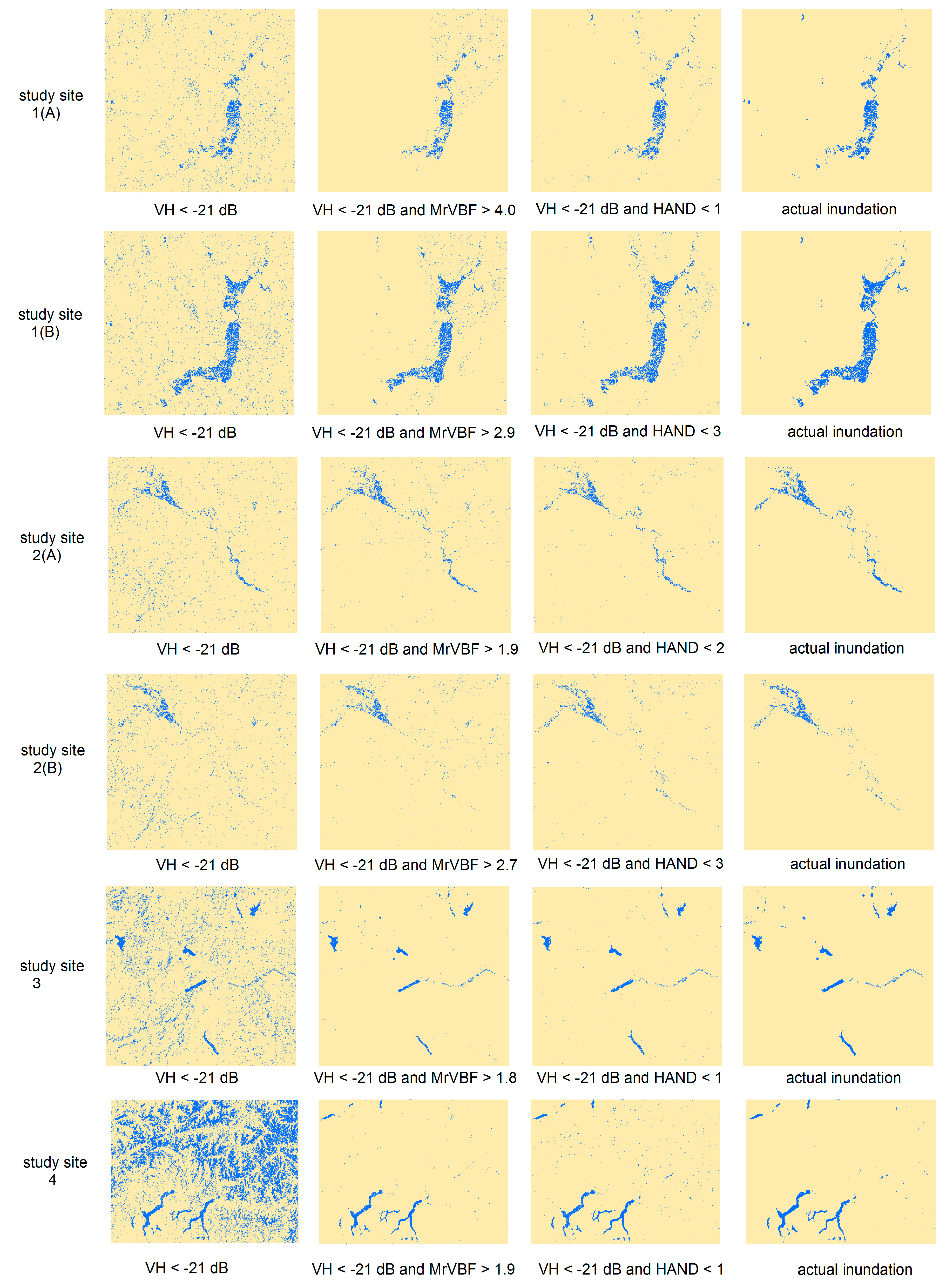
4.4. Optimal Thresholds and Their Performance

Based on the analysis in Section 4.3, optimal thresholds for different cases with different resolutions and different polarizations were identified and listed in

Table 3. Optimal thresholds and corresponding total disagreements (TDs).

Study Case	1s MrVBF (TD %)	1s HAND (TD %)	1s MrVBF (TD %)	1s HAND (TD %)	3s MrVBF (TD %)	3s HAND (TD %)	3s MrVBF (TD %)	3s HAND (TD %)
	VH Image		VV Image		VH Image		VV Image
Study site 1(A)	5.0 (1.253)	1 (1.165)	2.8 (1.096)	2 (0.965)	4.0 (1.514)	1 (1.354)	2.9 (1.259)	1 (1.149)
Study site 1(B)	3.9 (2.147)	2 (1.917)	2.8 (1.824)	3 (1.642)	2.9 (2.714)	3 (2.401)	1.9 (2.240)	4 (2.064)
Study site 2(A)	2.8 (0.943)	2 (0.824)	2.7 (0.716)	3 (0.665)	1.9 (1.124)	2 (0.954)	1.8 (0.859)	2 (0.782)
Study site 2(B)	2.9 (0.847)	3 (0.801)	2.9 (0.683)	3 (0.675)	2.7 (0.918)	3 (0.847)	1.9 (0.736)	3 (0.710)
Study site 3	2.0 (0.662)	6 (0.578)	1.1 (0.640)	8 (0.548)	1.8 (0.611)	1 (0.580)	0.9 (0.591)	5 (0.561)
Study site 4	2.0 (0.627)	1 (0.820)	2.0 (0.678)	1 (0.869)	1.9 (0.480)	1 (0.586)	0.9 (0.541)	1 (0.623)

. It is observed that using 3s resolution terrain indices to assist water mapping generally produces a higher TD than using 1s terrain indices, although the difference is very small. Water mapping results with the highest accuracies (lowest TD) for study sites 1(A), 1(B), 2(A), 2(B), and 3 used a 1s HAND image to mask VV based water extent with thresholds of 2, 3, 3, 3, and 8 m. While for study site 4, the best result was to mask VH based water extent with a threshold of 1.9 on 3s MrVBF image.

It is clear from Table 3 that based on VV or VH thresholding, with assistance from HAND or MrVBF, accurate water mapping can be achieved with TD less than 3%. Optimal thresholds for HAND are generally less than 4 m, optimal threshold for MrVBF varies depending on the study sites. For floodplain dominated study sites (1 and 2), optimal threshold is relatively higher than that for mountainous study sites.

For most of the cases in Table 3, VV based water maps seem to have slightly higher accuracy than VH based water maps. We notice that many studies [11,40] suggested that VH is better than VV in terms of water body detection, because VV’s higher sensitivity to wind-induced water surface condition makes it difficult to distinguish rough water surfaces and land. Our results suggest that the different performances of VV and VH are more similar than expected.

A series of water maps (Figure 9) were derived from VH polarization images assisted with 3s terrain index masks based on the optimal thresholds (bolded) in Table 3. Water maps without terrain mask, as well as actual water maps, were also displayed as references. As we can see from Figure 9, there are a lot of commission errors in the original VH thresholding maps. Most of these errors come from the terrain effect, which is even more obvious in mountainous sites. Through using either a MrVBF or HAND mask with an appropriate threshold, most of these errors were eliminated. The HAND mask looks slightly better than MrVBF mask in most of the cases except for study site 4.

5. Conclusions

SAR data can be quite useful for surface water mapping, but the data also have several disadvantages. Terrain effect is one of them that especially affects water mapping due to similar image values in terrain shadow regions and over water bodies. However, elevation information directly acquired from DEM is sometimes not suitable for assisting surface water mapping for two reasons. First, shadow areas could be located in low areas and water could be held in high places sometimes, which makes simply thresholding on elevation not reliable in delineating shadows and water bodies. Therefore, we need some kind of terrain index that has stronger connections with water presence than the original elevation. The second reason is that all DEMs have errors. However, when using terrain indices such as MrVBF and HAND, the absolute height error of DEM becomes less important, since we do not threshold against height in an absolute sense but rather are concerned with the valley bottom flatness, or relative spatial change in elevation, to quantify likely water presence.

This study conducted a comprehensive comparison on MrVBF and HAND toward their ability in assisting water mapping using Sentinel-1 C-band dual-polarized data. Through several case studies with different geomorphic types and inundation scenarios, we achieved the following three findings.

• Both terrain indices are able to help improve water mapping significantly. HAND performs slightly better than MrVBF in most of these cases.
• Optimal thresholds for both indices are not fixed. Adjustments are required to achieve optimal results. HAND is less sensitive to different thresholds, which is a good quality when being applied to larger areas with varied topography.
• MrVBF classifies low and flat areas with more details than HAND does. For example, those areas that have a unique HAND value of 0 may have quite different MrVBF values, depending on the scale of valley bottoms. This advantage makes MrVBF sometimes more effective in eliminating false water bodies in mountainous areas.

These findings are able to provide guidance for terrain index selection and usage when using DEM data for assisting surface water mapping from SAR imagery. It is suggested that for large scale or global water mapping, HAND index would be a better choice as the auxiliary data to SAR imagery. While for water mapping in complex terrain areas, MrVBF or a combination of MrVBF and HAND is recommended. Using either index, the threshold should be carefully selected to achieve optimal water mapping results. The results of this study are useful for other studies that apply SAR data for water mapping, either regionally or globally.

Though it has been proven that simply thresholding on either VV or VH polarized image with the assistance from terrain indices is able to derive water maps with high accuracy, we are aware that the results could be further improved with more advanced water detection algorithms. For example, it is believed that the rate of backscatter change with local incidence angle may provide a better means to map the water extents than a single threshold on backscatter alone [41]. Therefore, our future work will investigate robust water mapping methodologies that involve more variables, such as local incidence angle, terrain indices, or any other useful information.

References

1. World Bank. Earth Observation for Water Resources Management: Current Use and Future Opportunities for the Water Sector; World Bank Group: Washington, DC, USA, 2015. [Google Scholar]
2. Karpatne, A.; Khandelwal, A.; Chen, X.; Mithal, V.; Faghmous, J.; Kumar, V. Global monitoring of inland water dynamics: State-of-the-art, challenges, and opportunities. In Computational Sustainability; Lässig, J., Kersting, K., Morik, K., Eds.; Springer International Publishing: Cham, Switzerland, 2016; pp. 121–147. [Google Scholar]
3. Gao, H.; Zhang, S.; Durand, M.; Lee, H. Satellite remote sensing of lakes and wetlands. In Hydrologic Remote Sensing; CRC Press: Boca Raton, FL, USA, 2016; pp. 57–72. [Google Scholar]
4. McGinnis, D.; Rango, A. Earth resources satellite systems for flood monitoring. Geophys. Res. Lett. 1975, 2, 132–135. [Google Scholar] [CrossRef]
5. Westerhoff, R.; Kleuskens, M.; Winsemius, H.; Huizinga, H.; Brakenridge, G.; Bishop, C. Automated global water mapping based on wide-swath orbital synthetic-aperture radar. Hydrol. Earth Syst. Sci. 2013, 17, 651–663. [Google Scholar] [CrossRef]
6. Long, S.; Fatoyinbo, T.E.; Policelli, F. Flood extent mapping for Namibia using change detection and thresholding with SAR. Environ. Res. Lett. 2014, 9, 035002. [Google Scholar] [CrossRef]
7. Frison, P.L.; Paillou, P.; Sayah, N.; Pottier, E.; Rudant, J.P. Spatio-temporal monitoring of evaporitic processes using multiresolution C-band radar remote sensing data: Example of the Chott el Djerid, Tunisia. Can. J. Remote Sens. 2013, 39, 127–137. [Google Scholar] [CrossRef]
8. Di Baldassarre, G.; Schumann, G.; Brandimarte, L.; Bates, P. Timely low resolution SAR imagery to support floodplain modelling: A case study review. Surv. Geophys. 2011, 32, 255–269. [Google Scholar] [CrossRef]
9. Horritt, M.S.; Mason, D.C.; Luckman, A.J. Flood boundary delineation from synthetic aperture radar imagery using a statistical active contour model. Int. J. Remote Sens. 2001, 22, 2489–2507. [Google Scholar] [CrossRef]
10. Phuhinkong, P.; Kasetkasem, T.; Kumazawa, I.; Rakwatin, P.; Chanwimaluang, T. Unsupervised segmentation of synthetic aperture radar inundation imagery using the level set method. In Proceedings of the 11th International Conference on Electrical Engineering/Electronics, Computer, Telecommunications and Information Technology (ECTI-CON), Nakhon Ratchasima, Thailand, 14–17 May 2014. [Google Scholar]
11. Henry, J.B.; Chastanet, P.; Fellah, K.; Desnos, Y.L. Envisat multi-polarized ASAR data for flood mapping. Int. J. Remote Sens. 2006, 27, 1921–1929. [Google Scholar] [CrossRef]
12. White, L.; Brisco, B.; Dabboor, M.; Schmitt, A.; Pratt, A. A collection of SAR methodologies for monitoring wetlands. Remote Sens. 2015, 7, 7615–7645. [Google Scholar] [CrossRef]
13. Otsu, N. A threshold selection method from gray-level histograms. IEEE Trans. Syst. Man Cybern. 1979, 9, 62–66. [Google Scholar] [CrossRef]
14. Song, Y.-S.; Sohn, H.-G.; Park, C.-H. Efficient water area classification using RADARSAT-1 SAR imagery in a high relief mountainous environment. Photogram. Eng. Remote Sens. 2007, 73, 285–296. [Google Scholar] [CrossRef]
15. Wang, Y.; Colby, J.D.; Mulcahy, K.A. An efficient method for mapping flood extent in a coastal floodplain using Landsat TM and DEM data. Int. J. Remote Sens. 2002, 23, 3681–3696. [Google Scholar] [CrossRef]
16. Gianinetto, M.; Villa, P.; Lechi, G. Postflood damage evaluation using Landsat TM and ETM+ data integrated with DEM. IEEE Trans. Geosci. Remote Sens. 2006, 44, 236–243. [Google Scholar] [CrossRef]
17. Li, J.; Chen, W. A rule-based method for mapping Canada’s wetlands using optical, radar and DEM data. Int. J. Remote Sens. 2005, 26, 5051–5069. [Google Scholar] [CrossRef]
18. Pekel, J.-F.; Cottam, A.; Gorelick, N.; Belward, A.S. High-resolution mapping of global surface water and its long-term changes. Nature 2016, 540, 418–422. [Google Scholar] [CrossRef] [PubMed]
19. Gilbert, J.T.; Macfarlane, W.W.; Wheaton, J.M. The Valley Bottom Extraction Tool (V-BET): A GIS tool for delineating valley bottoms across entire drainage networks. Comput. Geosci. 2016, 97, 1–14. [Google Scholar] [CrossRef]
20. Jordan, G. Adaptive smoothing of valleys in DEMs using TIN interpolation from ridgeline elevations: An application to morphotectonic aspect analysis. Comput. Geosci. 2007, 33, 573–585. [Google Scholar] [CrossRef]
21. Williams, W.A.; Jensen, M.E.; Winne, J.C.; Redmond, R.L. An automated technique for delineating and characterizing valley-bottom settings. Environ. Monit. Assess. 2000, 64, 105–114. [Google Scholar] [CrossRef]
22. Hjerdt, K.N.; McDonnell, J.J.; Seibert, J.; Rodhe, A. A new topographic index to quantify downslope controls on local drainage. Water Resour. Res. 2004, 40, W05602. [Google Scholar] [CrossRef]
23. Gallant, J.C.; Dowling, T.I. A multiresolution index of valley bottom flatness for mapping depositional areas. Water Resour. Res. 2003, 39, 291–297. [Google Scholar] [CrossRef]
24. Mueller, N.; Lewis, A.; Roberts, D.; Ring, S.; Melrose, R.; Sixsmith, J.; Lymburner, L.; McIntyre, A.; Tan, P.; Curnow, S.; et al. Water observations from space: Mapping surface water from 25 years of Landsat imagery across Australia. Remote Sens. Environ. 2016, 174, 341–352. [Google Scholar] [CrossRef]
25. Chen, Y.; Huang, C.; Ticehurst, C.; Merrin, L.; Thew, P. An evaluation of MODIS daily and 8-day composite products for floodplain and wetland inundation mapping. Wetlands 2013, 33, 823–835. [Google Scholar] [CrossRef]
26. Huang, C.; Chen, Y.; Wu, J. Mapping spatio-temporal flood inundation dynamics at large river basin scale using time-series flow data and MODIS imagery. Int. J. Appl. Earth Obs. Geoinform. 2014, 26, 350–362. [Google Scholar] [CrossRef]
27. Rennó, C.D.; Nobre, A.D.; Cuartas, L.A.; Soares, J.V.; Hodnett, M.G.; Tomasella, J.; Waterloo, M.J. HAND, a new terrain descriptor using SRTM-DEM: Mapping terra-firme rainforest environments in Amazonia. Remote Sens. Environ. 2008, 112, 3469–3481. [Google Scholar] [CrossRef]
28. Nobre, A.D.; Cuartas, L.A.; Hodnett, M.; Rennó, C.D.; Rodrigues, G.; Silveira, A.; Waterloo, M.; Saleska, S. Height above the nearest drainage—A hydrologically relevant new terrain model. J. Hydrol. 2011, 404, 13–29. [Google Scholar] [CrossRef]
29. Donchyts, G.; Schellekens, J.; Winsemius, H.; Eisemann, E.; van de Giesen, N. A 30 m resolution surfacewater mask including estimation of positional and thematic differences using Landsat 8, SRTM and OpenStreetMap: A case study in the Murray-Darling basin, Australia. Remote Sens. 2016, 8, 386–407. [Google Scholar] [CrossRef]
30. Twele, A.; Cao, W.; Plank, S.; Martinis, S. Sentinel-1-based flood mapping: A fully automated processing chain. Int. J. Remote Sens. 2016, 37, 2990–3004. [Google Scholar] [CrossRef]
31. Schlaffer, S.; Chini, M.; Dettmering, D.; Wagner, W. Mapping wetlands in Zambia using seasonal backscatter signatures derived from ENVISAT ASAR time series. Remote Sens. 2016, 8, 402. [Google Scholar] [CrossRef]
32. Haile, A.T.; Rientjes, T. Effects of LiDAR DEM resolution in flood modelling: A model sensitivity study for the city of Tegucigalpa, Honduras. ISPRS Arch. 2005, XXXVI, 12–14. [Google Scholar]
33. Rabus, B.; Eineder, M.; Roth, A.; Bamler, R. The shuttle radar topography mission—A new class of digital elevation models acquired by spaceborne radar. ISPRS J. Photogramm. Remote Sens. 2003, 57, 241–262. [Google Scholar] [CrossRef]
34. Strozzi, T.; Wegmuller, U.; Wiesmann, A.; Werner, C. Validation of the X-SAR SRTM DEM for ERS and JERS SAR geocoding and 2-pass differential interferometry in alpine regions. In Proceedings of the 2003 IEEE International Geoscience and Remote Sensing Symposium, Toulouse, France, 21–25 July 2003. [Google Scholar]
35. Kääb, A. Combination of SRTM3 and repeat ASTER data for deriving alpine glacier flow velocities in the Bhutan Himalaya. Remote Sens. Environ. 2005, 94, 463–474. [Google Scholar] [CrossRef]
36. Sun, G.; Ranson, K.; Kharuk, V.; Kovacs, K. Validation of surface height from shuttle radar topography mission using shuttle laser altimeter. Remote Sens. Environ. 2003, 88, 401–411. [Google Scholar] [CrossRef]
37. O’Callaghan, J.F.; Mark, D.M. The extraction of drainage networks from digital elevation data. Comput. Vis. Graph. Image Proc. 1984, 28, 323–344. [Google Scholar] [CrossRef]
38. Sabel, D.; Bartalis, Z.; Wagner, W.; Doubkova, M.; Klein, J.-P. Development of a global backscatter model in support to the Sentinel-1 mission design. Remote Sens. Environ. 2012, 120, 102–112. [Google Scholar] [CrossRef]
39. Pontius, R.G.; Millones, M. Death to Kappa: Birth of quantity disagreement and allocation disagreement for accuracy assessment. Int. J. Remote Sens. 2011, 32, 4407–4429. [Google Scholar] [CrossRef]
40. Schumann, G.; Matgen, P.; Hoffmann, L.; Hostache, R.; Pappenberger, F.; Pfister, L. Deriving distributed roughness values from satellite radar data for flood inundation modelling. J. Hydrol. 2007, 344, 96–111. [Google Scholar] [CrossRef]
41. O’Grady, D.; Leblanc, M.; Gillieson, D. Relationship of local incidence angle with satellite radar backscatter for different surface conditions. Int. J. Appl. Earth Obs. Geoinform. 2013, 24, 42–53. [Google Scholar] [CrossRef]
Figure 1. Study sites and their locations.
Ijgi 06 00140 g001
Figure 2. Flowchart of Multi-resolution Valley Bottom Flatness (MrVBF) calculation. DEM, Digital Elevation Model.
Ijgi 06 00140 g002
Figure 3. Flowchart of Height Above Nearest Drainage (HAND) calculation.
Ijgi 06 00140 g003
Figure 4. One arc-second (1s) and three arc-second (3s) Shuttle Radar Topographic Mission (SRTM) DEM data for all four study sites, along with MrVBF and HAND images derived from them.
Ijgi 06 00140 g004
Figure 5. Histograms of normalized MrVBF and HAND images.
Ijgi 06 00140 g005
Figure 6. Scatterplots of normalized MrVBF and HAND values.
Ijgi 06 00140 g006
Figure 7. Boxplots of MrVBF and HAND values in water areas.
Ijgi 06 00140 g007
Figure 8. Disagreement of 3s terrain indices masked results for different study cases, disagreement of non-masked results (constant horizontal line) were shown for reference.
Ijgi 06 00140 g008
Figure 9. Water maps from VH polarization based on 3s terrain index masking using optimal thresholds, together with no terrain masking and actual water maps.
Ijgi 06 00140 g009