Integration of Landscape Metrics and Variograms to Characterize and Quantify the Spatial Heterogeneity Change of Vegetation Induced by the 2008 Wenchuan Earthquake

Abstract

The quantification of spatial heterogeneity can be used to examine the structure of ecological systems. The 2008 Wenchuan earthquake caused severe vegetation damage. In addition to simply detecting change, the magnitude of changes must also be examined. Remote sensing and geographic information system techniques were used to produce landscape maps before and after the earthquake and analyze the spatial-temporal change of the vegetation pattern. Landscape metrics were selected to quantify the spatial heterogeneity in a categorical map at both the class and landscape levels. The results reveal that the Wenchuan earthquake greatly increased the heterogeneity in the study area. In particular, forests experienced the most fragmentation among all of the landscape types. In addition, spatial heterogeneity in a numerical map was studied by using variogram analysis of normalized difference vegetation indices derived from Landsat images. In comparison to before the earthquake, the spatial variability after the earthquake had doubled. The structure of the spatial heterogeneity represented by the range of normalized difference vegetation index (NDVI) variograms also changed due to the earthquake. Moreover, the results of the NDVI variogram analysis of three contrasting landscapes, which were farmland, broadleaved forest, and coniferous forest, confirm that the earthquake produced spatial variability and changed the structure of the landscapes. Regardless of before or after the earthquake, farmland sites are the most heterogeneous among the three landscapes studied.

1. Introduction

The 2008 Wenchuan earthquake, which occurred on 12 May and had a magnitude of 8.0 Ms according to the China Earthquake Administration, caused great damage to infrastructure and resulted in human fatalities. Moreover, many natural resources were destroyed during the earthquake. In addition to the direct destruction and devastation wrought by the earthquake itself, the ensuing secondary disasters, such as landslides and debris flows, were also responsible for the horrifying aftermath [1,2,3,4]. All of these disturbances consequently impacted the ecosystem. However, existing studies have mainly focused on the spatial distribution of the damaged vegetation [5,6] or quantitatively estimated the spatial-temporal variations in vegetation recovery [7,8]; none of these studies conducted a structural analysis of the vegetation. This study aims to provide such complementary information in terms of spatial heterogeneity.

Spatial heterogeneity is one structural feature of ecological systems. It can be defined as the complexity and variability of a system property in time and space. A system property in this case can be almost any measurable entity, such as the configuration of the landscape mosaic, plant biomass, annual precipitation, and soil nutrient concentrations [9,10]. Li [9] proposed operational definitions for spatial heterogeneity in both categorical and numerical landscape maps. Spatial heterogeneity in categorical landscape maps is defined as the complexity for both the composition (which is non-spatial) and configuration (which is spatial) of a patch. Composition addresses which categories are present and how much of the categories are present, while ignoring the specific spatial arrangement of the categories on the landscape. Configuration refers to the specific spatial arrangement of the different cover types on a landscape.

For variability of spatial heterogeneity, Burrough [11] proposed that spatial heterogeneity in numerical landscape maps is a continuum of degrees of variability in domain variation, autocorrelated variation, and random noise. Garrigues et al. [12] provided detailed definitions of the variability of spatial heterogeneity measured from remote sensing sensors, which is described through the following two components: (1) spatial variability of the surface property over the observed scene and (2) spatial structures. The components are defined as patches or objects that repeat themselves independently within the observed scene at a characteristic length scale that represents the extent of the spatial structure. They can be viewed as the typical correlation area of the surface property. Spatial structures within remotely sensed images are identifiable because their spectral properties are more homogeneous within them than between them. Other data of scene elements are often distributed into independent sets of spatial structures, related to different length scales and spatial variability being overlaid in the same region.

To monitor ecosystem changes before and after the earthquake at the landscape scale, we must quantify the system structure of interest to determine the magnitude and rate of change [13,14]. Quantification of spatial heterogeneity is a promising way to examine the structure of ecological systems [15]. The fundamental premise is that spatial heterogeneity may have great effects on the functions and processes of ecological systems, and these changes in spatial heterogeneity may reflect changes in functions and processes [10,16,17,18].

Accordingly, in this paper, we used categorical and numerical maps to quantify and analyze changes in the spatial heterogeneity that were caused by the earthquake. This type of analysis can offer a comprehensive understanding of the spatial heterogeneity change in the study area and provide a theoretical basis for future sustainable forest management and local development. Moreover, the results of this study may also be useful for researchers studying the habitats of giant pandas (Ailuropoda melanoleuca), which inhabit the study site.

2. Materials and Methods

2.1. StudyArea

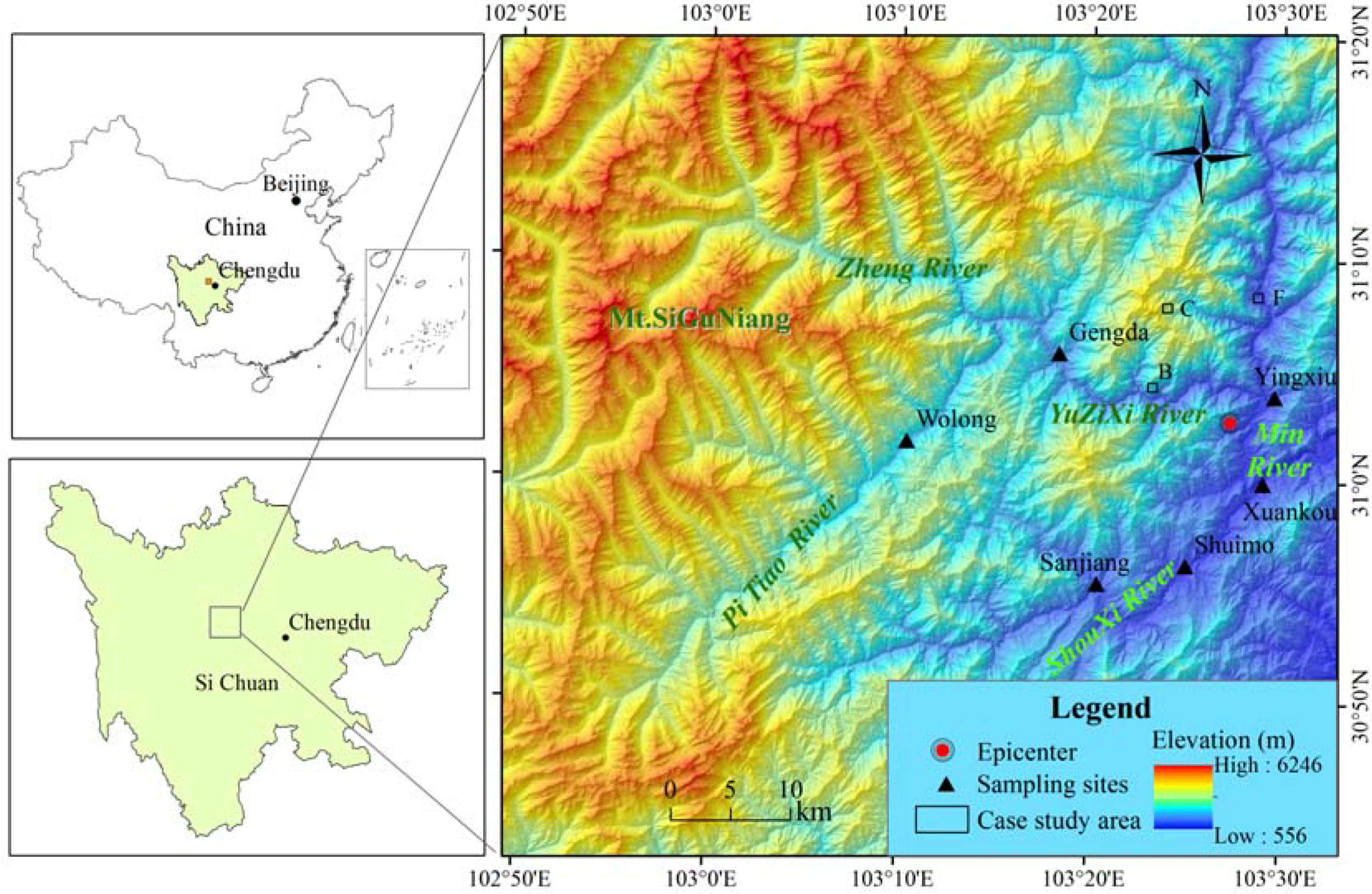
We selected the Yingxiu area, which includes Yinxiu town, Wolong Nature Reserve, and Sanjiang Reserve, and is situated near the epicenter of the Wenchuan earthquake, as a study area (Figure 1). This area supplies water and other ecological services to the dry valley of upper Minjiang River, which has various land-use types. However, it is also an ecologically fragile area of western China. The study area covers 6600 km² and contains two watersheds, Yuzixi and Shouxi, which are the two main tributaries of the Min River. Yuzixi River originates in Mt. Balang with a flow direction of west to east, a total length of 89 km, and a basin area of 1742 km². It passes through the Wolong Nature Reserve and Yinxiu town, before finally flowing into the Min River. The source of the Shouxi River is located on Mt. Menkan. It flows through Sanjiang Nature Reserve, Shuimo town, and Xuankou town into the Min River and has a total length of 65 km and a total area of 596 km².

The study area is generally mountainous, as shown by the digital elevation model (DEM) in Figure 1, with high mountains over 6000 m above sea lever, such as Mt. Siguniang (6250 m). The Pitiao River acts as a boundary limit between west and south as well as west and east, as the northwestern corner of the investigated area is characterized by high elevation topography for the western and northwestern areas.

2.2. Remotely Sensed Data Processing

Remote sensing and geographic information system techniques have been shown to be useful for environmental monitoring that seeks to detect land cover change at various scales [5,19,20]. Remote sensing techniques used in the present study mainly consisted of preprocessing satellite images and vegetation classification using the module of ISODATA (Iterative Self-Organizing Data Analysis Technique) unsupervised classification of ENVI 4.5 (IDL) image-processing software. Spatial variability analysis and vegetation structure data were implemented with a variogram using a modular of geostatistical analyst in ArcGIS 10 (ESRI). In addition, an intersection of the two landscape maps in order to prepare the transfer matrix was also conducted using ArcGIS.

2.3. Data Resources and Preprocessing

The data consisted of satellite images, topographic maps with a scale of 1:250,000, a 25-m digital elevation model (DEM), and ground observations. Four scenes of Landsat-7 enhanced thematic mapper (ETM+) data sets (Rows 38 and 39/Path 130 of WRS-2) acquired on 5 April 2008 and 23 May 2008 were used to classify the vegetation type before and after the earthquake. The ETM+ sensor measures the Earth’s surface reflectance of electro-magnetic waves from the Sun’s illumination at the following seven spectral bands: visible blue (0.45–0.52 μm), green (0.52–0.60 μm), red (0.63–0.69 μm), near-infrared (0.76–0.90 μm), shortwave infrared (1.55–1.75 and 2.08–2.35 μm), thermal infrared (10.5–12.5 μm), and panchromatic mode (0.52–0.90 μm).

These remote sensing images were first orthorectified based on the available raster DEM and then geo-referenced to the universal transverse Mercator coordinate system Zone 48 North with other related data. Two adjacent scenes of the geo-referenced ETM+ images for each time were merged to one scene and clipped to the study area.

2.4. Vegetation Type Map

A hybrid unsupervised-supervised approach of image classification [21,22,23] was applied to the ETM+ image data to characterize the main vegetation types of the study area before and after the earthquake. This approach is a combination of two procedures, ISODATA (Iterative Self-Organizing Data Analysis Technique) and maximum-likelihood. Fifteen spectral clusters were identified using the ISODATA. All image pixels were then classified into one of the clusters using maximum-likelihood. Several clusters were identified as belonging to one vegetation type through interactive interpretation. Classes were defined to match six categories of the main vegetation types in the study area that existed before the earthquake occurred: coniferous forest; broadleaved forest; meadow; farmland; shrub; and another class for non-vegetation features, such as snow, ice, and water bodies. The image classification for the post-earthquake was a combination of pre-earthquake classification and a ruined area detected by a decrease of normalized difference vegetation index (NDVI) values. The resultant vegetation map was assessed using kappa coefficient, which is widely used in classification accuracy of remote sensing images. The value 0.81 for all classes is satisfactory for the objectives of this study. In addition, we checked the classification results by three-time field investigations in five towns in 2008. The survey sites were shown in Figure 1. We took around 150 pictures with GPS positions for local landscapes in these towns and on the ways to the towns. We simply compared the survey result with the classification result and found about 85% agreement. The higher accuracy than the kappa coefficient may be due to the pictures that were mostly taken at the areas severely damaged by the earthquake.

2.5. Landscape Metrics

To examine the complexity of spatial heterogeneity in categorical landscape maps, several landscape metrics were employed both for composition and configuration analysis. Fragstats 3.3 was the software utilized to calculate the landscape metrics selected in this study. Landscape metrics are commonly defined at the following three levels: patch level metrics, class level metrics, and landscape level metrics. In this study, the analysis was performed at both the class and landscape levels. Class level indices separately quantify the amount and spatial configuration of each patch type and thus provide a means to quantify the extent and fragmentation of each patch type in the landscape. Landscape level metrics are integrated over all patch types or classes over the full extent of the data.

An extensive set of landscape metrics was used in this study [23,24]. We evaluated the following indices in both class level and landscape level: Total (Class) Area (CA/TA), Number of Patches (NP), Patch Density (PD), Largest Patch Index (LPI), Landscape Shape Index (LSI), Patch Richness (PR), Clumpiness Index (CLUMPY), Shannon’s Diversity Index (SHDI), Perimeter-Area Fracture Dimension (PAFRAC), Shannon’s Evenness Index (SHEI), and Contagion (CONTAG). These metrics were chosen because they are commonly used in landscape ecology to represent different spatial heterogeneity components [23,24,25]. The equations and ecological significance of each index are modified from Fragstats [26].

2.6. Geostatistical Techniques

Geostatistical techniques were employed to investigate the relationship between fracture zones and vegetation patterns. Geostatistics are spatial statistics used to explore the correlation and dependence between spatial variables based on regionalized variable theories [27]. Geostatistics include the following two techniques: variograms, which model spatial dependence, and kriging, which provides estimates for unsampled locations. A fundamental assumption of geostatistics is that any two sample locations separated by a similar distance and direction should have a similar squared difference of data values. This relationship is called stationarity. Garrigues [12] reviewed several spatial tools, such as local variance, fractal, spatial entropy, variogram, Fourier transform, and wavelet transform, which can characterize spatial heterogeneity of landscape vegetation cover, and concluded that NDVI variograms were most appropriate for this purpose.

Normalized difference vegetation index (NDVI) has been demonstrated to be a useful indicator of overall green biomass, canopy closure, tree density, and tree species diversity and has the following formula:

$$\mathrm{NDVI}=\frac{{\mathrm{R}}_{NIR}-{\mathrm{R}}_{RED}}{{\mathrm{R}}_{NIR}+{\mathrm{R}}_{RED}}$$

(1)

where R_RED and R_NIR are the reflectance at visible red and near-infrared bands, respectively. Although NDVI is sensitive to soil and atmospheric effects, it is a good indicator of the vegetation amount [28]. Moreover, the topographic effect on the NDVI can usually be disregarded [29], which makes it more valuable in studies of mountainous areas.

In this paper, NDVI data were considered as a regionalized variable z(x). At first, the experimental variogram was computed in the NDVI image domain, which measures the average squared differences between values z(x_α) and z(x_β) of paired pixels (x_α, x_β) separated by vector h (Equation (2)).

$${\mathsf{\gamma }}_{\mathrm{e}}(h)=\frac{1}{2N(h)}{{\displaystyle \sum _{\left(x_{\alpha }-x_{\beta }\right)=h}\left\{z\left(x_{\alpha }\right)-z\left(x_{\beta }\right)\right\}}}^2$$

(2)

If a spatial correlation exists, pairs of points that are closer together should have more similar values. At a large distance, it may reach a sill that is an indicator of the spatial variability of the data. The range is the distance that the experimental variogram reaches the sill. Pairs of locations beyond the range are considered to be uncorrelated. A discontinuity of the experimental variogram at the origin, termed the nugget effect, can be caused by either uncorrelated noise (measurement error) or nested spatial structures at a scale smaller than the pixel size.

To provide a parametric characterization of spatial heterogeneity, a theoretical variogram is estimated by fitting a valid mathematical function to the experimental variogram [27]. In this study, the spherical model is used because it suited the main properties of the experimental variograms (Equation (3)).

$$\mathsf{\gamma }(h)={\sigma }^2\left(\frac{3}{2}\frac{h}{r}-\frac{1}{2}{\left(\frac{h}{r}\right)}^3\right)$$

(3)

Spatial autocorrelation that depends only on the distance between two locations is called isotropy. Directional influence in γ(h) that yields different autocorrelation values at the same distance depending on direction is called anisotropy. If anisotropy exits in NDVI γ(h), the vegetation pattern is bound to be the highest continuity along the direction of the major range. Therefore, the NDVI γ(h) is capable of characterizing vegetation patterns.

3. Results

3.1. Spatial Heterogeneity Characteristics in Terms of a Categorical Map

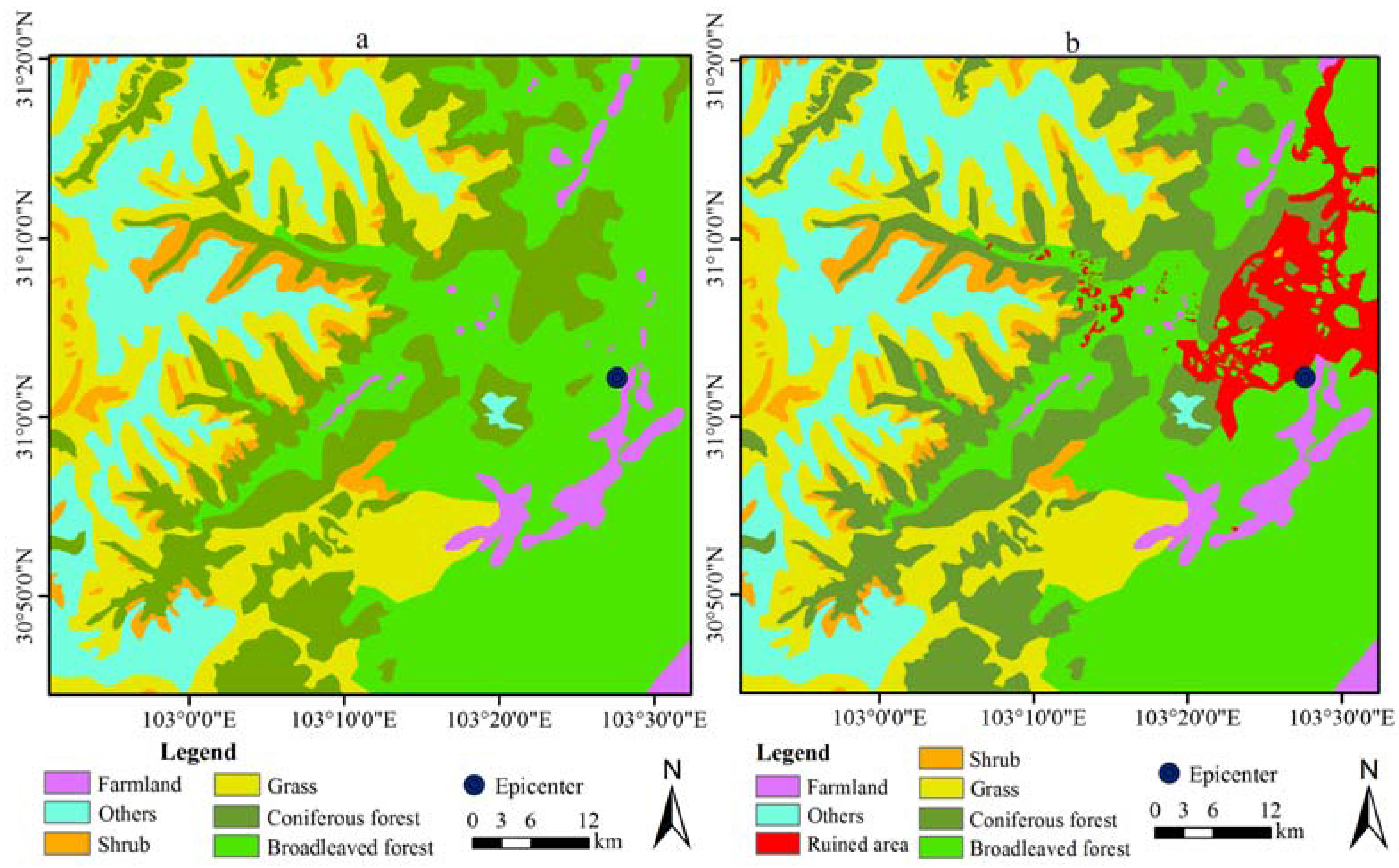
The structure of the alpine environment is often characterized by assessing the pattern and composition of plant productivity and cover type information [21,30]. Landscape types in the study area consisted of coniferous forest, broadleaved forest, deciduous forest, mixed forest, farmland, and others (ice, snow, and bare land) before the earthquake (Figure 2a); for after the earthquake, an additional landscape type, namely, the ruined area, was used to discriminate areas destroyed by the earthquake from normal non-vegetated areas (Figure 2b).

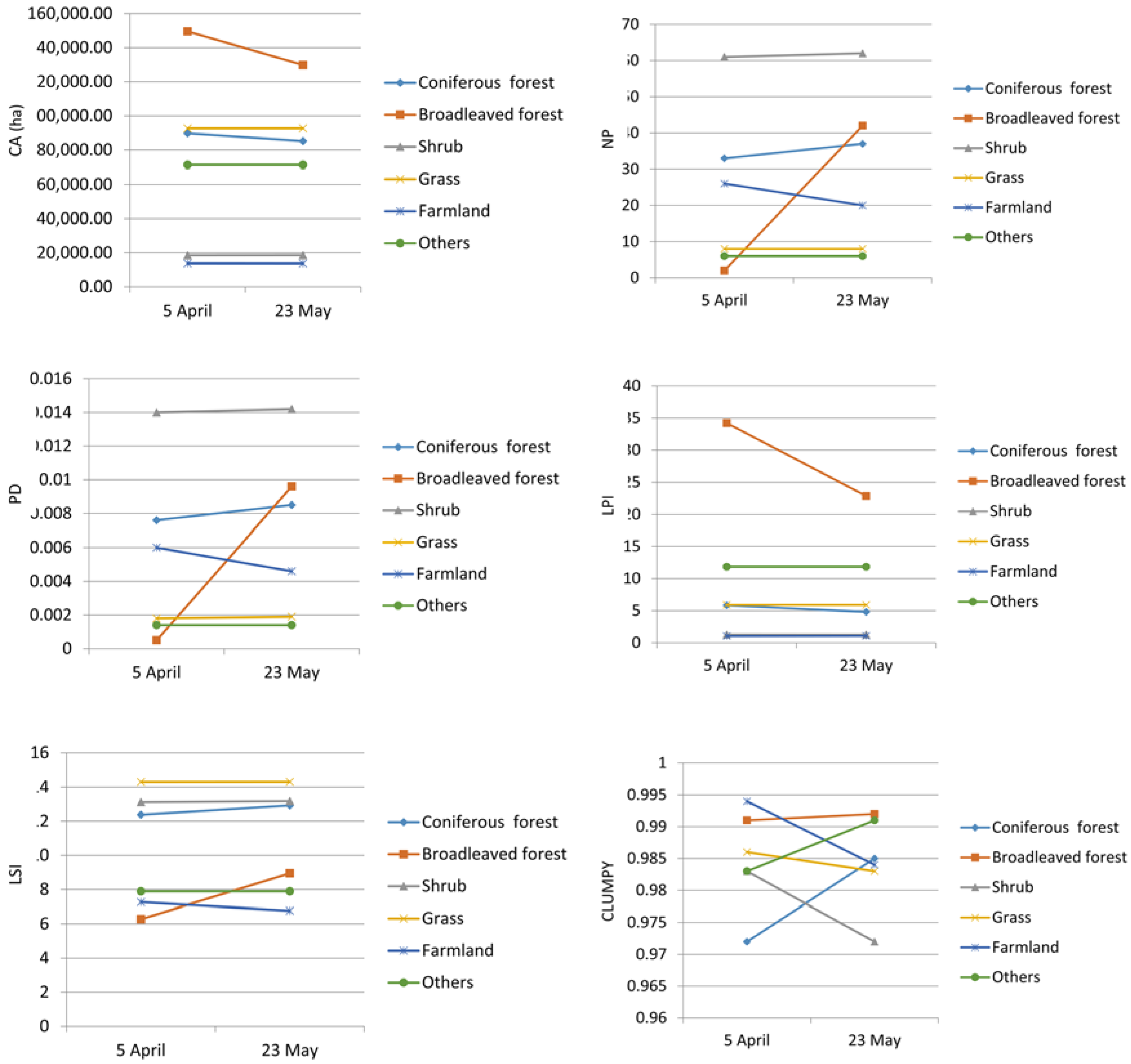
Six landscape metrics were utilized to quantify the spatial heterogeneity before and after the earthquake at both the class and landscape levels. The spatial heterogeneity of each landscape type was well characterized and is presented in

Table 1. Characteristics of spatial heterogeneity of vegetation at class level before and after the earthquake. CA, Class Area; NP, Number of Patches; PD, patch density; LPI, Largest Patch Index; LSI, Landscape Shape Index; CLUMPY, Clumpiness Index.

Landscape Type	Date	Landscape Metrics
		CA	NP	PD	LPI	LSI	CLUMPY
Coniferous forest	5 April	89,724.87	33	0.0076	5.8417	12.3791	0.972
	23 May	85,148.55	37	0.0085	4.8101	12.9306	0.985
Broadleaved forest	5 April	149,590.40	2	0.0005	34.2206	6.2757	0.991
	23 May	129,797.50	42	0.0096	22.8653	8.9413	0.992
Shrub	5 April	18,595.26	61	0.0140	1.2891	13.1253	0.983
	23 May	18,661.14	62	0.0142	1.2782	13.1855	0.972
Grass	5 April	92,625.57	8	0.0018	5.8972	14.3041	0.986
	23 May	92,660.04	8	0.0019	5.8972	14.3103	0.983
Farmland	5 April	13,713.93	26	0.0060	1.0478	7.2650	0.994
	23 May	13,654.42	20	0.0046	1.0723	6.7641	0.984
Others	5 April	71,349.75	6	0.0014	11.8423	7.8928	0.983
	23 May	71,349.75	6	0.0014	11.8423	7.8928	0.991
Ruined area	5 April	-	-	-	-	-	-
	23 May	24,917.58	51	0.0117	5.44	8.8623	0.984

and Figure 3. The area of broadleaved forest was 149,590.4 hectares, ranking the largest among all landscape types, followed by grass and coniferous forest, respectively (Table 1). The landscape type areas after the earthquake had the same order as before the earthquake, although the areas of coniferous forest and broadleaved forest decreased and shrub and grass area increased. The area of farmland decreased a little after the earthquake (Figure 3). Most of the landscape component types increased in patch number, especially broadleaved forest, which increased from 2 to 42 after the earthquake (Table 1). The change in the patch density showed the same pattern among the landscape types with patch number. The Clumpiness value for all classes changed negligibly in comparing the conditions before and after the earthquake.

The largest patch index refers to the area of the largest patch of the corresponding patch type. It is an indicator of dominance for all the landscape types. All the classes changed negligibly or remained the same, except for the broadleaved forest, which decreased sharply from 34.22 to 22.87. The values of the broadleaved forest were the highestboth before and after the earthquake, demonstrating its dominance in the area. A decrease of the largest patch index also showed that the areas were fragmented. This same trend can also be found in the coniferous forest.

The landscape shape index equaled 1 when the landscape consists of a single square or a maximally compact (i.e., almost square) patch of the corresponding type; LSI increased without limit as the patch type became more disaggregated. According to Table 1 and Figure 3, the value of the landscape shape index increased for all forest types, implying that all forest types became more disaggregated after the Wenchuan earthquake.

Table 2. Spatial heterogeneity change of vegetation at landscape level before and after the earthquake. CONTAG, Contagion; PR, Patch Richness; SHDI, Shannon’s Diversity Index; SHEI, Shannon’s Evenness Index.

Date	Landscape Type
	NP	PD	LPI	LSI	PAFRAC	CONTAG	PR	SHDI	SHEI
5 April 2008	136	0.03	34.22	12.04	1.37	58.21	6	1.56	0.87
23 May 2008	226	0.05	22.86	13.71	1.27	54.16	7	1.71	1.17

summarizes the results of landscape metrics selected to quantify spatial heterogeneity of the study area at the landscape level. Each of the indices represents a different type of measure of spatial heterogeneity change after the earthquake.

To understand how each landscape type changed after the earthquake, a transfer matrix was constructed (

Table 3. Transfer matrix of each vegetation type before and after the earthquake.

5 April 2008	23 May 2008
	Coniferous Forest	Broadleaved Forest	Shrub	Grass	Farmland	Others	Ruined Area	Total
Coniferous forest	838.57	13.83	0.66	4.27	-	-	45.33	902.65
Broadleaved forest	12.85	1277.57	-	0.71	2.12	-	210.16	1503.40
Shrub	-	-	185.96	2.03	-	-	-	188.00
Grass	-	0.36	1.88	927.18	-	-	0.67	930.09
Farmland	-	4.91	-	-	128.56	-	4.14	137.61
Others	-	-	-	-	-	713.42	-	713.42
Total	851.42	1296.67	188.50	934.19	130.68	713.42	260.30	4375.17

). A total of 210 km² of broadleaved forest and 45 km² of coniferous forest were transformed to bare land. Relatively littlefarmland and grass area was damaged.

3.2. NDVI Variogram Analysis

For variogram analysis, the average NDVI values of all pairs with a similar distance and angle were plotted on a variogram surface, as shown in Figure 4. An ellipse was overlaid on each variogram surface to represent the range at each direction; flatness of the ellipse increased with increasing anisotropic strength of the variogram. Figure 4a,b show γ(h)s along the major and minor axes. Clearly, NDVIγ(h)s before and after the earthquake can be adequately approximated by a spherical model (Figure 4a,b). All NDVIγ(h)s before and after the earthquake are linear at the origin, and all converge to sills.

Table 4. Parameters of variogram models innormalized difference vegetation index(NDVI) experimental variograms for the whole study area.

Date	Model	Sill	Nugget Effect	Minor Range (m)	Major Range (m)	Direction of Major Range
5 April 2008	Spherical	0.015	0.016	21,000	35,000	N33°E
23 May 2008	Spherical	0.039	0.028	25,000	40,000	N30°E

summarizes the parameters of the variogram models. The spatial variability is represented by the summation of the sill and nugget effect. Before the earthquake, the spatial variability was 0.031. After the earthquake, the spatial variability increased to 0.067, which is more than twice than that before the earthquake.

The structure of spatial heterogeneity can be characterized by the range of the variogram. According to the results summarized in Table 3 and Figure 4c, both the minor and major range of the NDVI variogram increased after the earthquake, from 21 km to 25 km and from 35 km to 40 km, respectively. In terms of anisotropy, before the earthquake, the γ(h) greatly increased near the origin and reached the sill at the major range along the direction of N33°E. After the earthquake, the γ(h) reached the sill at the major range along the direction of N30°E and demonstrated a slight change in comparison to before the earthquake.

In particular, we examined the spatial heterogeneity of three contrasted landscapes (broadleaved forest, coniferous forest, and farmland) by modeling the variograms in three areas of the case study. As shown in

Table 5. Parameters of variogram models in NDVI experimental variograms for three contrasting landscapes, including broadleaved forest, coniferous forest, and farmland.

Landscapes	Nugget Effect		Sill		Range (m)
	5 April	23 May	5 April	23 May	5 April	23 May
Broadleaved forest	0.0001	0	0.0038	0.071	202	512
Coniferous forest	0.001	0.002	0.0064	0.015	298	379
Farmland	0.002	0.001	0.0094	0.022	474	284

, all three land-use types had higher sill values after the earthquake than before the earthquake. In comparison to the natural forest, which was broadleaved forest and coniferous forest in this case, farmland had the highest sill value both before and after the earthquake. Comparatively, broadleaved forest had lower sill values than coniferous forest.

4. Discussion

4.1. Spatial Heterogeneity Changes at the Scale of Class Level

Class-lever metrics can be used to quantify spatial heterogeneity of each vegetation type. They have been well applied to the study of habitat fragmentation, which is a process in which the contiguous habitat is progressively sub-divided into smaller, geometrically more complex, and more isolated habitat fragments as a result of both natural processes and human land use activities [26]. This process involves changes in landscape composition, structure, and function, and occurs on a backdrop of a natural patch mosaic created by changing landforms and natural disturbances. In our study, we first quantified such changes created by the earthquake. Six types of landscape metrics were calculated on landscape maps before and after the earthquake to measure the change of each category. CA measures how much of one particular patch type is present in the whole landscape. Forests are the main component type in our study area. Our results showed that all kinds of forest decreased from the earthquake, though the changing magnitudes were more or less different. Broadleaved forest was most affected out of all of the types of forest. Broadleaved forest was widely distributed near the epicenter of the earthquake. Several studies have documented that vegetation damage was negatively correlated with elevation with the exception of the 1500–2500 m elevation, where the broadleaved forest widely exists [5,7]. By calculating the change percentage of each landscape type to the area damaged by the earthquake, we found that up to 14% of broadleaved forests were destroyed during the earthquake. Coniferous forest ranked second, with a destroyed magnitude of 5%.

The number of patches of a particular patch type is a simple measure of the extent of subdivision or fragmentation of the patch type. The largest increase of patch number was observed in the forest (i.e., coniferous forest and broadleaved forest) among all landscape types after the earthquake, suggesting that considerable fragmentation of the forest was caused by the earthquake. The same trend was found for patch density. Out of the different landscape types, broadleaved forest had the most patch area, but the smallest patch number and density of patches before the earthquake, indicating that broadleaved forest is the main landscape type in this study area. Such an extensive area of broadleaved forest must play an important role in the function of the ecosystem. However, due to the earthquake, the area of broadleaved forest was fragmented, as indicated by the patch number that greatly increased from 2 to 42. Habitat loss and fragmentation is the prevalent trajectory of landscape change, and it is increasingly recognized as a major cause of declining biodiversity [31,32]. Therefore, the fragmentation caused by the Wenchuan earthquake is most likely to have affected the ecosystem in some way.

4.2. Spatial Heterogeneity Changes at the Landscape Level Scale

Nine types of landscape level metrics were selected to measure the change of landscape before and after the earthquake in terms of composition and configuration.

Patch richness is the simplest measure for landscape composition. The total patch number increased from 136 to 226 after the earthquake, indicating that the Wenchuan earthquake extremely aggravated the spatial heterogeneity in this area (Table 2). The value of the largest patch index also decreased greatly. Landscape level metrics corresponded to all patch types over the whole area, with no sensitivity to a single class. An increase of the largest shape index indicates that the cover type tends to occur in isolated, dispersed grid cells or small patches.

Contagion measures aggregation of patch types. The relatively high value of contagion before the earthquake indicates that the patch types were better aggregated than after the earthquake. Due to the earthquake, the contagion value decreased from 58 to 54. Shannon’s diversity index measures the diversity of patch types. The value of SHDI increased from 1.56 to 1.71 after the earthquake, which was due to the patch richness increasing from 6 to 7. Shannon’s evenness index increased, which may be due to the earthquake destroying some cover types, decreasing their dominance in the area. Perimeter-area fractal dimension measures irregularity of patch shape in a landscape. Perimeter-area fractal dimension measures irregularity of patch shape in a landscape. Our results suggested that the patch shape tended to be more regular by the effect of earthquake, as proved by the decrease in PAFRAC value.

Quantifying the ecosystem structure is one of the demands for monitoring ecosystem change at the regional scale [10]. Spatial heterogeneity is one such structural feature of ecological systems. The changes of spatial heterogeneity may be linked to functional responses of species to them. Li and Reynolds [9] ran a simulation model to examine the effectiveness of landscape indices to measure spatial heterogeneity. Different indices express different components of spatial heterogeneity. The evenness index reflects the proportion of patch types, which determines the dominance (or lack) of critical resources. Fractal dimension reflects heterogeneity components of both spatial arrangement and patch shape, which may affect species dispersal and foraging efficiency. Contagion responds to all heterogeneity components. A clear difference of landscape merits was confirmed by comparing the results before and after the earthquake, indicating more fragmented habitat for species, especially for giant panda.

The sill value of NDVI γ(h) can measure the magnitude of spatial variability of vegetation. The parameters listed in Table 4 show that the sill on 23 May 2008 was larger than that on 5 April 2008, indicating that the spatial variability of vegetation pattern after the earthquake was greater than before the earthquake. However, the minor range increased from 21 km before the earthquake to 25 km after the earthquake. The spatial correlations of NDVI on 23 May 2008 were stronger and longer than those of 5 April 2008, when comparing the shapes of γ(h)s. This result suggested that the earthquake uniformly decreased vegetation growth over a wide area. The sills of NDVIγ(h)s of the study area increased from 0.015 to 0.039 before and after the earthquake, respectively, suggesting that the Wenchuan earthquake caused the vegetation pattern to become more heterogeneous, mainly by changing the vegetation cover to bare land. Results for the broadleaved forest, coniferous forest, and farmland confirm that the spatial heterogeneity increased after the earthquake. Garrigues [12] found that crop sites are more heterogeneous than natural vegetation and forest sites at the landscape level, which is consistent with our results. Broadleaved forest has the lowest sill among the three contrasting landscapes because the vegetation development and presence of green understory limit the variability of the landscape vegetation cover. The high variability of farmland is explained by the mosaic of vegetation field with high NDVI values and relatively bare soil field (boundary of no crops) with low NDVI values. The shape of the variograms provides an understanding of the NDVI spatial structures within the image domain. In regard to the three landscape types, both broadleaved forest and coniferous forest have a larger structure after the earthquake, which is consistent with the whole study area. However, the variogram of farmland shows that smaller spatial structures survived after the earthquake. The structure of farmland is related to the mosaic of the agricultural fields. Apparently, the earthquake fragmented these crop fields into smaller ones. As shown by the whole study domain and the three landscapes, the variogram of the NDVI proved to be a powerful tool to characterize and quantify the spatial variability of the vegetation pattern.

5. Conclusions

In this study, we quantified the spatial heterogeneity that occurred after the Wenchuanearthquake and analyzed the changes of this spatial heterogeneity. We integrated the methods of landscape indices and variograms based on categorical maps and numerical maps, respectively.

Vegetation maps before and after the earthquake were produced as data for quantifying spatial heterogeneity in terms of a categorical map. Ten landscape metrics were selected to quantify the spatial heterogeneity at both the class and landscape levels. The class level results indicated that forests were the most fragmented from the earthquake. The results from the landscape level revealed that the earthquake greatly affected the spatial heterogeneity; the whole landscape was more heterogeneous, the dominance decreased, and the patch shape was more irregular.

NDVI variograms were used to quantify the spatial heterogeneity in terms of the variability of change and spatial structure. It can be concluded from our results that the Wenchuan earthquake resulted in twice the variability than before the earthquake. Due to much of the vegetation changing to bare land, the range of the NDVI variogram increased after the earthquake, indicating evident change in the structure of spatial heterogeneity.

The variograms were additionally applied to three contrasting landscapes, farmland, broadleaved forest, and coniferous forest, to characterize and quantify each of their spatial heterogeneity. The farmland site is the most heterogeneous among the three landscapes, as shown by the different NDVI values found between crops fields and the mosaic of relatively bare soil fields. Natural forest sites, such as the broadleaved forest and coniferous forest, are more homogeneous than crops site because of their green understory. The results of the comparison before and after the earthquake for the three case studies confirm that the earthquake led to spatial variability and structure change. The bare soil mosaics caused by the earthquake explain most of the variability at these sites.

References

- Huang, R.; Li, W. Development and distribution of geohazards triggered by 5.12 Wenchuan earthquake in China. Sci. China Ser. E Technol. Sci. 2008, 52, 810–819. [Google Scholar] [CrossRef]
- Chigira, M.; Wu, X.; Inokuchi, T.; Wang, G. Landslides induced by the 2008 Wenchuan earthquake, Sichuan, China. Geomorphology 2010, 118, 225–238. [Google Scholar] [CrossRef]
- Tang, H.; Jia, H.; Hu, X.; Li, D.; Xiong, C. Characteristics of landslides induced by the great Wenchuan earthquake. J. Earth Sci. 2010, 21, 104–113. [Google Scholar] [CrossRef]
- Fan, J.; Chen, J.; Tian, B. Rapid assessment of secondary disasters induced by the Wenchuan earthquake. Comput. Sci. Eng. 2010, 12, 10–19. [Google Scholar] [CrossRef]
- Wang, L.; Tian, B.; Masoud, A.; Koike, K. Relationship between Remotely Sensed Vegetation Change and Fracture Zones Induced by the 2008 Wenchuan Earthquake, China. J. Earth Sci. 2013, 24, 282–296. [Google Scholar] [CrossRef]
- Peng, W.; Wang, G.; Zhou, J.; Xu, X.; Luo, H.; Zhao, J.; Yang, C. Dynamic monitoring of fractional vegetation cover along Minjiang River fromWenchuan County to Dujiangyan City using multi-temporal landsat 5 and 8 images. Acta Ecol. Sin. 2016, 36, 1975–1988. [Google Scholar]
- Jiao, Q.; Zhang, B.; Liu, L.; Li, Z.; Yue, Y.; Hu, Y. Assessment of spatio-temporal variations in vegetation recovery after the Wenchuan earthquake using Landsat data. Nat. Hazards 2014, 70, 1309–1326. [Google Scholar] [CrossRef]
- Xu, J.; Tang, B.; Lu, T. Monitoring the riparian vegetation cover after the Wenchuan earthquake along the Minjiang River valley based on multi-temporal Landsat TM images: A case study of the Yingxiu-Wenchuan section. Acta Ecol. Sin. 2013, 33, 4966–4974. [Google Scholar]
- Li, H.; Reynolds, J.F. A simulation experiment to quantify spatial heterogeneity in categorical maps. Ecology 1994, 75, 2446–2455. [Google Scholar] [CrossRef]
- Turner, M.G.; Gardner, R.H. (Eds.) Quantitative Methods in Landscape Ecology; Springer: New York, NY, USA, 1991. [Google Scholar]
- Burrough, P. Principles of geographical information systems for land resources assessment. Geocarto Int. 1986, 1. [Google Scholar] [CrossRef]
- Garrigues, S.; Allard, D.; Baret, F. Quantifying spatial heterogeneity at the landscape scale using variogram model. Remote Sens. Environ. 2006, 103, 81–96. [Google Scholar] [CrossRef]
- O’Neill, R.V.; Krummel, J.R.; Gardner, R.H.; Sugihara, G.; Jackson, B.; DeAngelis, D.L.; Milne, B.T.; Turner, M.G.; Zygmunt, B.; Christensen, S.W.; et al. Indices of landscape pattern. Landsc. Ecol. 1988, 1, 153–162. [Google Scholar] [CrossRef]
- TurnerM, G. Spatial and temporal analysis of landscape patterns. Landsc. Ecol. 1990, 4, 21–30. [Google Scholar] [CrossRef]
- O’Neill, R.V.; Gardner, R.H.; Sugihara, G.; Milne, B.T.; Turner, M.G.; Jackson, B. Heterogeneity and spatial hierarchies. In Ecological Heterogeneity; Springer: New York, NY, USA, 1991; pp. 85–96. [Google Scholar]
- Risser, P.G.; Karr, J.R.; Forman, R.T.T. Landscape Ecology: Directions and Approaches; Special Publication 2; Illinois Natural History Survey: Champaign, IL, USA, 1984; p. 18. [Google Scholar]
- Forman, R.T.T.; Godron, M. Landscape Ecology; John Wiley & Sons: New York, NY, USA, 1986; p. 619. [Google Scholar]
- Kolasa, J.; Pickett, S.T.A. (Eds.) Ecological Heterogeneity; Springer: New York, NY, USA, 1991. [Google Scholar]
- Wang, L.; Duan, B.; Zhang, Y.; Berninger, F. Net primary production of Chinese fir plantation ecosystems and its relationship to climate. Biogeosciences 2014, 11, 5595–5606. [Google Scholar] [CrossRef]
- Tian, B.; Wang, L.; Kashiwaya, K.; Koike, K. Combination of Well-Logging Temperature and Thermal Remote Sensing for Characterization of Geothermal Resources in Hokkaido, Northern Japan. Remote Sens. 2015, 7, 2647–2667. [Google Scholar] [CrossRef]
- Brown, D.; Danial, G. Predicting vegetation types at treeline using topography and biophysical disturbance. J. Veg. Sci. 1994, 5, 641–656. [Google Scholar] [CrossRef]
- Jensen, J. Introductory Digital Image Processing: A Remote Sensing Prospective, 2nd ed.; Prentice Hall: Englewood Cliffs, NJ, USA, 1996; p. 318. [Google Scholar]
- Turner, M.G.; Gardner, R.H.; O’Neill, R.V. Landscape Ecology in Theory and Practice: Pattern and Processes; Springer: New York, NY, USA, 2001; p. 404. [Google Scholar]
- MacGarical, K.; Marks, B.J. FRAGSTAT: Spatial Pattern Analysis Program for Quantifying Landscape Structure; General Technical Report PNW-GTR-351; US Department of Agriculture, Forest Service, Pacific Northwest Research Station: Portland, OR, USA, 1995; p. 122.
- Costantini, M.; Zaccarelli, N.; Mandrone, S.; Rossi, D.; Calizza, E.; Rossi, L. NDVI spatial pattern and the potential fragility of mixed forested areas in volcanic lake watersheds. For. Ecol. Manag. 2012, 285, 133–141. [Google Scholar] [CrossRef]
- McGarigal, K.; Cushman, S.; Neel, M.; Ene, E. FRAGSTATS: Spatial Pattern Analysis Program for Categorical Maps; Computer Software Program: Amherst, MA, USA, 2002; Available online: http://www.umass.edu/landeco/research/fragstats/fragstats.html (accessed on 1 June 2016).
- Journel, A.G.; Huijbregts, C. Mining Geostatistics; Academic Press: San Diego, CA, USA, 1978; p. 600. [Google Scholar]
- Henebry, G. Detecting change in grasslands using measures of spatial dependence with Landsat TM. Remote Sens. Environ. 1993, 46, 233–234. [Google Scholar] [CrossRef]
- Matsushita, B.; Yang, W.; Chen, J. Sensitivity of the Enhanced Vegetation Index (EVI) and Normalized Difference Vegetation Index (NDVI) to topographic effect: A case study in high-density cypress forest. Sensors 2007, 7, 2636–2651. [Google Scholar] [CrossRef]
- Walsh, S.J.; Butler, D.R.; Brown, D.G.; Bian, L. Form and pattern of alpine environments: An integrative approach to spatial analysis and modelling in Glacier National Park, USA. In Mountain Environments and GIS; Heywood, D.I., Price, M.F., Eds.; Taylor and Francis: London, UK, 1994; pp. 189–672. [Google Scholar]
- Segan, D.; Murray, K.; Watson, J. A global assessment of current and future biodiversity vulnerability to habitat loss-climate change interactions. Glob. Ecol. Conserv. 2016, 5, 12–21. [Google Scholar] [CrossRef]
- Niebuhr, B.; Wosniack, M.; Santos, M.; Raposo, E.; Viswanathan, G.; Daluz, M.; Pie, M. Survival in patchy landscapes: The interplay between dispersal, habitat loss and fragmentation. Sci. Rep. 2015, 5, 11898. [Google Scholar] [CrossRef] [PubMed]
Figure 1.
Location map of the study area Yingxiu near the epicenter of the Wenchuan earthquake on 12 May 2008, and topographic features of a digital elevation model with 25 m resolution from the national topographic database of China. For the case study area, F denotes farmland, C denotes coniferous forest, and B denotes broadleaved forest.
Figure 2.
Vegetation type maps interpreted from two images of Landsat enhanced thematic mapper (ETM+) data before (5 April 2008) and after (23 May 2008) the Wenchuan earthquake. Vegetation type map (a) before the earthquake and (b) after the earthquake.
Figure 3.
Spatial heterogeneity change of each vegetation type at class level as quantified by landscape metrics at the corresponding level.
Figure 4.
Experimental variograms of NDVI data calculated from two images of Landsat ETM+ data before (5 April 2008) and after (23 May 2008) the Wenchuan earthquake at the study area. Variograms (a) along the major range and (b) along the minor range; and (c) variogram surfaces when plotting the average values of data pairs separated by similar distances (shown by the distance from the center) and angle at each azimuth (0–360°). Curves on the variograms express spherical models that approximate the trends. Ellipses on the variogram surfaces indicate the range for each direction.