Pan-Sharpening of Landsat-8 Images and Its Application in Calculating Vegetation Greenness and Canopy Water Contents

Abstract

Pan-sharpening is the process of fusing higher spatial resolution panchromatic (PAN) with lower spatial resolution multispectral (MS) imagery to create higher spatial resolution MS images. Here, our overall objective was to pan-sharpen Landsat-8 images and calculate vegetation greenness (i.e., normalized difference vegetation index (NDVI)), canopy structure (i.e., enhanced vegetation index (EVI)), and canopy water content (i.e., normalized difference water index (NDWI))-related variables. Our proposed methods consisted of: (i) evaluating the relationships between PAN band (0.503–0.676 µm) with a spatial resolution of 15 m and individual MS bands of Landsat-8 from blue (i.e., acquiring in the range 0.452–0.512 µm), green (i.e., 0.533–0.590 µm), red (i.e., 0.636–0.673 µm), near infrared (NIR: 0.851–0.879 µm), shortwave infrared-I (SWIR-I: 1.566–1.651 µm), and SWIR-II (2.107–2.294 µm) bands with a spatial resolution of 30 m; (ii) determining the suitable individual MS bands to be enhanced into the spatial resolution of the PAN band; and (iii) calculating several vegetation greenness and canopy moisture indices (i.e., NDVI, EVI, NDWI-I, and NDWI-II) at 15 m spatial resolution and subsequent validation using their equivalent-values at a spatial resolution of 30 m. Our analysis revealed that strong linear relationships existed between the PAN and most of the MS individual bands of interest except NIR. For example, r² values were 0.86–0.89 for blue band; 0.89–0.95 for green band; 0.84–0.96 for red band; 0.71–0.79 for SWIR-I band; and 0.71–0.83 for SWIR-II band. As a result, we performed smoothing filter-based intensity modulation method of pan-sharpening to enhance the spatial resolution of 30 m to 15 m. In calculating the vegetation indices, we used the enhanced MS images and resampled the NIR to 15 m. Finally, we evaluated these indices with their equivalents at 30 m spatial resolution and observed strong relationships (i.e., r² values in the range 0.98–0.99 for NDVI, 0.95–0.98 for EVI, 0.98–1.00 for NDWI).

1. Introduction

Pan-sharpening is one of the branches of data fusion that has recently received increasing attention in the remote sensing community. It aims at fusing images acquired over multiple spectral bands with relatively low spatial resolution and a panchromatic (PAN) image with relatively high spatial resolution, resulting in the spectral resolution of the former and the spatial resolution of the latter [1,2]. Thus, the procedures refer to the fusion of a PAN and multispectral (MS) images simultaneously acquired over the same area. Information captured with different spatial and spectral resolution from air-borne, space-borne, and remotely installed camera systems can be fused by panchromatic band and can be enhanced into higher spatial resolution by following the pan-sharpening technique. The PAN band is a single spectral band that usually expands at least two or more visible and/or near infrared (NIR) bands. As a result, PAN band provides the opportunity to enhance the spatial resolution of MS bands by using pan-sharpening techniques. This is advantageous in a way that systems can be designed with lower bandwidth and storage requirements [3]. Also, MS bands with lower spatial resolution can allow for increased spectral resolution in the event of an appropriate PAN band when designing future imaging systems. General characteristics of the pan-sharpening technique imply the improvement of spatial resolution of multispectral bands using spatial information extracted from PAN band of higher spatial resolution. The pan-sharpening method is commonly used for visualization, allowing small details to be observed on multispectral images [4]. The application is highly regarded to understand more details of built-up areas [5], land surface temperature [6], land cover classification [7], large-area settlement patterns [8], wetland and forest classification [9], crop suitability assessment at higher resolution [10,11], ecological indicators [12], ice mapping [13], and vegetation indices [14,15]. As a result, it has become more significant for researchers to have higher resolution imageries to calculate several vegetation indices since high-resolution PAN images became available in February 2013 [16].

In contemporary literature, most of the pan-sharpening techniques follow a general protocol, such as: (i) extraction of high-frequency spatial information from the PAN image and (ii) injection of such spatial details into the resampled MS bands by exploiting different models [17]. Among the many popular pan-sharpening techniques, some of the important techniques are also identified in several literature sources [18,19,20,21,22,23,24,25,26,27,28,29,30]. Those include:

• The Intensity, Hue, Saturation (IHS) method, which is described as the conversion of color image from RGB (Red, Green, Blue) space into the IHS color space [18,19]. Because the intensity band resembles a PAN image in the fusion, a reverse IHS transform is then performed on the PAN together with the hue and saturation bands, resulting in an IHS fused image. When the PAN band is not highly correlated with the low spatial resolution bands, then the radiometric distortion of the color composite is quite obvious [20]. Typically, this method uses the high-resolution PAN image to replace the intensity component and obtains the fused image by applying an inverse IHS transform [21].
• The Principal Component Analysis (PCA) transform converts inter-correlated MS bands into a new set of uncorrelated components [22,23,24]. The first component also resembles a Pan image. It is, therefore, replaced by a high spatial resolution Pan for the fusion. The Pan image is fused into the low spatial resolution MS bands by performing a reverse PCA transform.
• The Brovey Transform (BT), Synthetic Variable Ratio (SVR), and Ratio Enhancement (RE) techniques are also used with a mathematical combination of the color image and high resolution data [25]. The procedures of the Brovey Transform first multiplies each MS band by the high resolution PAN band and then divides each product by the sum of the MS bands. The SVR and RE techniques are similar but involve more sophisticated calculations for the MS sum for better fusion quality. Usually, the Brovey transform, SVR, and RE have been developed to visually increase contrast in the low and high ends of an image’s histogram. In general, BT is a combination of arithmetic operations and it needs to normalize the spectral bands before they are multiplied with the PAN band [26,27].
• In wavelet fusion, a high spatial resolution Pan image is first decomposed into a set of low resolution Pan images with corresponding wavelet coefficients (spatial details) for each level [11,28]. Individual bands for the MS image then replace the low spatial resolution Pan at the resolution level of the original MS image. The high resolution spatial detail is injected into each MS band by performing a reverse wavelet transform on each MS band together with the corresponding wavelet coefficient.
• In UNB pan sharp, the algorithm utilises the least squares technique to find the best fit between the grey values of the PAN and the MS bands to adjust the contribution of individual bands to the fusion result [29]. It usually employs a set of statistical approaches to estimate the grey value relationship between all the input bands to eliminate the problem of data dependency.
• The Smoothing Filter-based Intensity Modulation (SFIM) fusion algorithm points out that by using a ratio between a higher resolution image and its low-pass filtered (with a smoothing filter) image, spatial details can be modulated to a co-registered lower resolution MS image without altering its spectral properties and contrasts [28].
• Other methods are also incorporated in literature with special emphasis on local mean and variance matching (LMVM); least square fusion methods, local mean matching fusion method, and the Gram-Schimdt fusion method. All of these techniques have been used to increase the spatial and spectral resolution of MS bands using PAN band [18,30].

Even though several pan sharpening techniques have been employed and reported in the literature, some common limitations have been identified. Those include: (i) quality color distortion in the fused images [22]; (ii) skills and knowledge of the persons employed in doing the fusion [31]; (iii) quality results are rarely obtained [18]; and (iv) building the relationships of individual MS bands with the PAN image [32]. Note that most of the platforms acquire PAN images in the spectrum ranging between 0.50–0.90 µm (that spans visible and NIR bands). Some of the well-known satellites include: SPOT 1/2/3 HRV, SPOT 5 HRG, IRS 1C, IRS 1D, Landsat 7 ETM+, IKONOS, QuickBird, and OrbView, among others. However, the new member of the Landsat series, i.e., Landsat-8 OLI (capturing the details of the earth’s surface since February 2013) has a PAN band operational over 0.503–0.676 µm. As it differs from the other PAN bands in terms of wavelength and/or spectral resolution, it is critical and challenging to evaluate how this band of interest can be utilized in enhancing the spatial resolution of NIR spectral bands in particular.

The overall objective of this study was to pan-sharpen Landsat-8 images and calculate vegetation greenness (i.e., normalized difference vegetation index (NDVI)), canopy structure (i.e., enhanced vegetation index (EVI)), and canopy water content (i.e., normalized difference water index (NDWI))-related variables. In fact, we attempted to fulfill these in three consecutive steps. Firstly, we evaluated relationships between PAN band (0.503–0.676 µm) with a spatial resolution of 15 m and individual MS bands of Landsat-8 from blue (i.e., acquired in the range 0.452–0.512 µm), green (i.e., 0.533–0.590 µm), red (i.e., 0.636–0.673 µm), NIR (i.e., 0.851–0.879 µm), shortwave infrared-I (SWIR-I: 1.566–1.651 µm), and SWIR-II (2.107–2.294 µm) bands with a spatial resolution of 30 m. Secondly, we used the obtained relationships from the first step to determine the suitable individual MS bands to be enhanced into the spatial resolution of the PAN band. Finally, we calculated several vegetation greenness and canopy moisture indices (i.e., NDVI, EVI, NDWI-I, and NDWI-II) at 15 m spatial resolution and validated this using their equivalent-values at a spatial resolution of 30 m. Note that researchers performed pan-sharpening in order to enhance the spatial resolution of both red and NIR spectral bands and subsequently to calculate NDVI-values [10,11]. In fact, the major issue was not having an appropriate level of evaluation of the suitability of the NIR spectral band to be PAN sharpened, which was one of the considerations in the scope of this paper (i.e., first step as mentioned earlier).

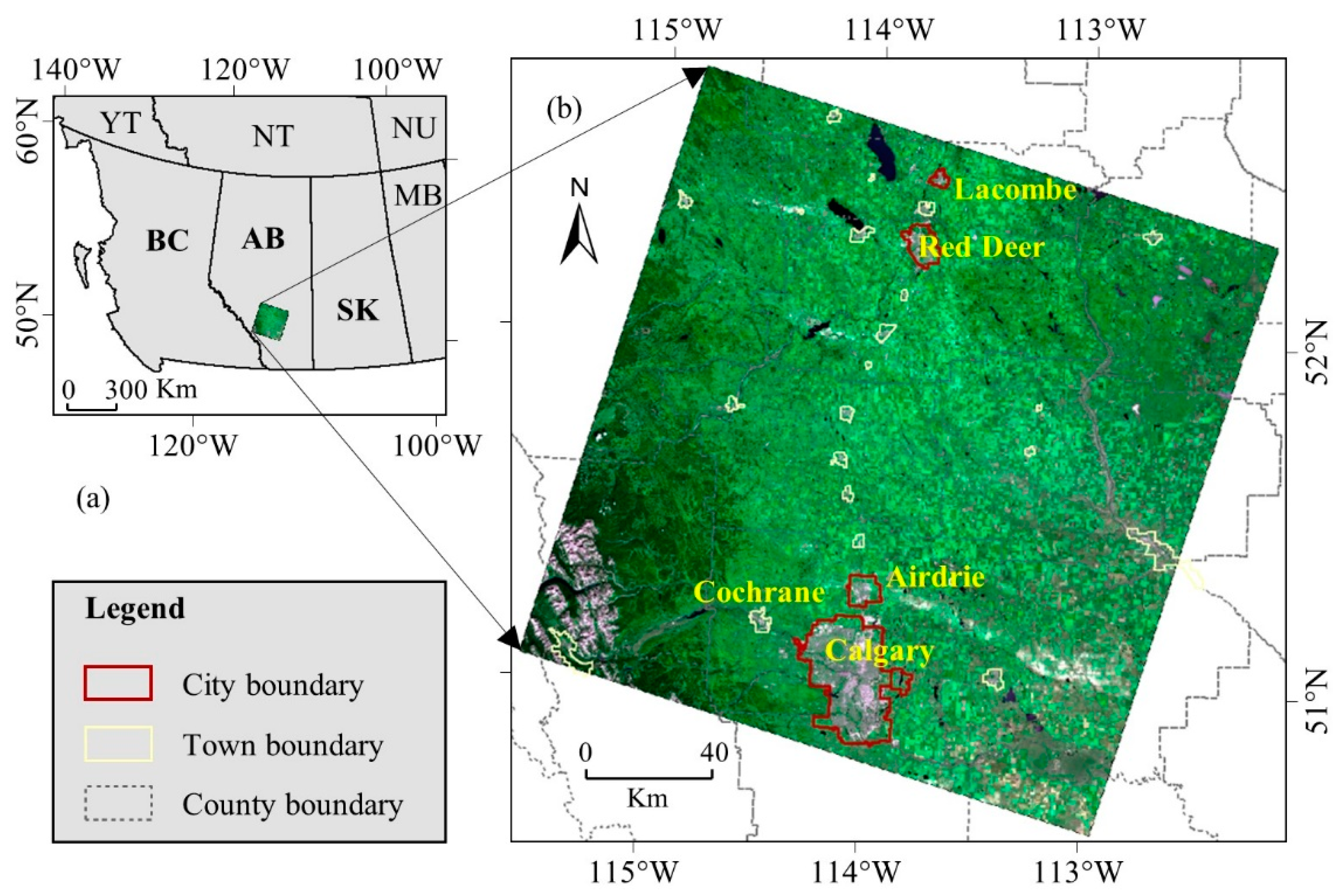
2. Study Area and Data Requirements

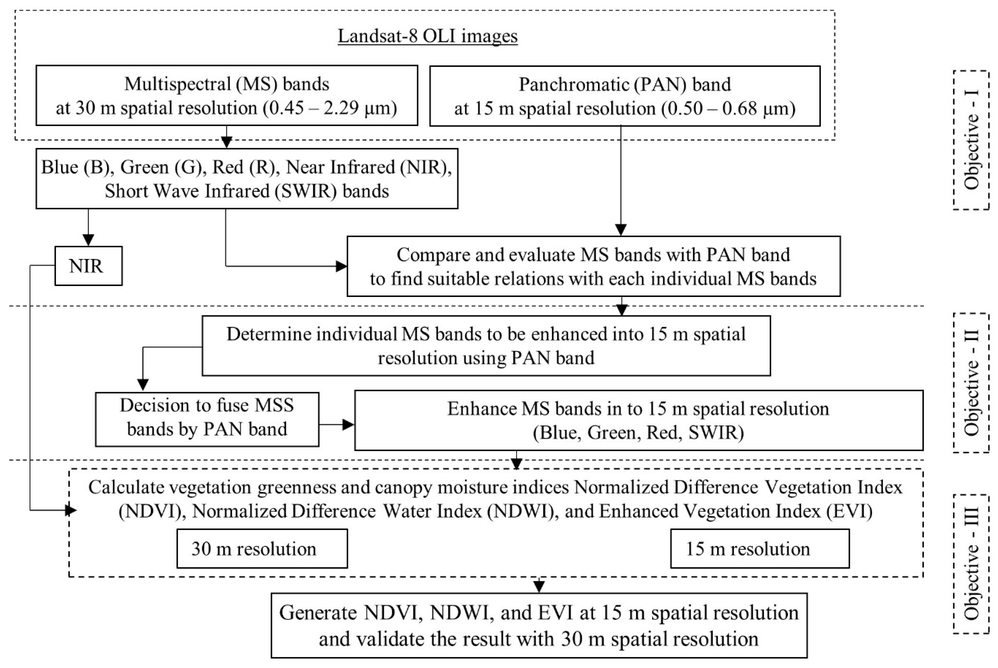
Here, we consider the southern part of the province of Alberta, Canada, as our study area. This area comprises a major city Calgary, some smaller cities (i.e., Cochrane, Airdrie, and Chestermere), and small townships within the single image captured through the Landsat-8 OLI satellite. The area is located between 50° and 52° North and 113° and 115° West and covers approximately 37,772 km² (Figure 1). The area is mostly covered with built up areas, agricultural land, forests, and water bodies. The major North-South corridor (Edmonton and Calgary corridor) passes through this area with a major highway along with small townships. Climatically, the study area experiences relatively cold (i.e., yearly average air temperature in the range of −3.6 to 1.1 °C) and dry (i.e., annual average precipitation varies between 377–535 mm) conditions [33,34].

In this study, we used Landsat-8 OLI images captured on different dates since July 2013 as Landsat-8 has been acquiring images since March 2013. The Landsat-8 OLI platform provided images in MS bands (that include blue, green, red, NIR, SWIR wavelengths) at 30 m spatial resolution, PAN band at 15 m, and Thermal Infrared Sensor (TIRS) band at 100 m. The data characteristics of these satellite images included: (i) Geo TIFF data format, i.e., a public domain metadata standard that allowed geo-referencing information to be embedded within a TIFF file); (ii) Cubic convolution resampling; (iii) Universal Transverse Mercator (UTM) map projection system; and (iv) World Geodetic System (WGS) 84 datum. Note that WGS 84 is an Earth-centered, Earth-fixed terrestrial reference system and geodetic datum which is based on a consistent set of constants and model parameters that describe the Earth’s size, shape, and gravity and geomagnetic fields. We collected these data on the basis of little (less than 1%) to no cloud contamination for further consideration and analysis. We finalized the data to be analyzed for the following days: 24 August 2013, 10 July 2014, 11 August 2014, and 27 June 2015.

3. Methods

Figure 2 illustrates the employed methods in this study in the form of a schematic diagram. The methods consisted of three major parts: (i) collecting the Landsat-8 OLI data and comparing the relationships among MS and PAN bands, (ii) determining the individual MS bands to be enhanced with the help of PAN band, and (iii) generating NDVI, NDWI, and EVI at 15 m spatial resolution. These are briefly described in the following sub-sections.

3.1. Collection of Landsat-8 OLI Data and Evaluation of the Relationships among MS and Pan Bands

We obtained the Landsat-8 OLI images from the United States Geological Survey (USGS) and its collaboration organization National Aeronautics and Space Administration (NASA) website on some specific days (as mentioned in the study area and data requirements section). Once the data were available, we re-projected the images into UTM zone 12 projection with datum NAD83. Then, we stored these images and converted them into Geo-TIFF format for further analysis.

Once we pre-processed the acquired images as described above, we started to assess the relationships between PAN and each of the individual MS bands using linear regress analysis. As a result, we obtained fitness between the variables of interest by means of calculating the coefficient of determination (i.e., r²) using the following expression:

$$r^2={\left[\frac{{\displaystyle \sum }\left(M{S}_i-{\overline{MS}}_i\right)\left(\mathrm{PAN}-\overline{PAN}\right)}{\sqrt{{\displaystyle \sum }{\left(M{S}_i-{\overline{MS}}_i\right)}^2}\sqrt{{\displaystyle \sum }{\left(\mathrm{PAN}-\overline{PAN}\right)}^2}}\right]}^2$$

(1)

where i represents the specific MS band of interest; MS and $\overline{MS}$ represent instantaneous and average surface reflectance values, respectively, for the specific band of interest; and PAN and $\overline{PAN}$ represent instantaneous and average digital number (DN)-values, respectively, for the PAN band. It is interesting to note that we found strong relationships between PAN and almost all of the MS bands except the NIR band (see details for “Results and Discussion” section).

3.2. Data Fusion (Pan-Sharpening)

After determining the relationships among several MS bands and PAN band as described in the previous sub-section, we took the decision to pan-sharpen the MS bands blue, green, red, SWIR-I, and SWIR-II. In order to execute the pan-sharpening process, we performed the following two steps as described in [35] and implemented in [23]. Firstly, we generated a synthetic image known as “Synthetic Pan” image (Syn_PAN) as a function of averaging of the PAN image over a moving kernel of n × n size (i.e., 3 × 3 in this study). Here, we opted to consider a 3 × 3 moving window in order to retain the local variabilities of the reflectance regimes. Secondly, we employed the Syn_PAN image in conjunction with PAN and specific MS bands (MS_i) in order to generate pan-sharpened MS bands of interest (i.e., Fused_i). Mathematically, we summarized both of the steps as follows:

$$Syn{ }_{PAN@15 m}= \frac{1}{n}{\displaystyle \sum }_1^{n}PAN@15 m$$

(2)

$$Fused{ }_{i@15 m}= \frac{PAN@15 m}{Syn{ }_{PAN}@15 m}*M{S}_{i@30 m}$$

(3)

where i represents the specific MS band of interest.

3.3. Generation of Vegetation and Canopy Moisture Contents and Their Validation

Upon pan-sharpened MS bands, we calculated a set of vegetation indices (i.e., NDVI and EVI) and canopy moisture content-related indices (i.e., NDWI) at 15 m spatial resolution using the following expressions:

$$NDVI=\frac{{\rho }_{NIR}-{\rho }_R}{{\rho }_{NIR}+{\rho }_R}$$

(4)

$$EVI=G*\frac{{\rho }_{NIR}-{\rho }_R}{{\rho }_{NIR}+C_1*{\rho }_R-C_2*{\rho }_B+L}$$

(5)

$$NDWI=\frac{{\rho }_{NIR}-{\rho }_{SWIR}}{{\rho }_{NIR}+{\rho }_{SWIR}}$$

(6)

where ρ represents surface reflectance for the specific MS band of interest. In these calculations, we resampled the NIR band from 30 m to 15 m in order to match other pan-sharpened MS bands. In the event of NDWI, we calculated this twice as the considered SWIR bands consisted of two different spectral resolutions (i.e., central wavelengths (centred at 1.64 µm and 2.20 µm).

In addition, we also calculated the NDVI, EVI, and NDWI at 30 m spatial resolution, which were then used to validate their equivalent-values produced at 15 m. In the process of validation, we applied linear regression analysis (that provided slope and intercept) and calculated r² and root mean square error (RMSE) values using the following expressions:

$$r^2={\left[\frac{{\displaystyle \sum }\left(A_x-{\overline{A}}_x\right)\left(B_x-{\overline{B}}_x\right)}{\sqrt{{\displaystyle \sum }{\left(A_x-{\overline{A}}_x\right)}^2}\sqrt{{\displaystyle \sum }{\left(B_x-{\overline{B}}_x\right)}^2}}\right]}^2$$

(7)

$$\mathrm{RMSE}=\sqrt{\frac{{\displaystyle \sum }[B_x-A_x{]}^2}{n}}$$

(8)

where x represents the specific indices; A and $\overline{A}$ represent instantaneous and average indices-specific values, respectively, at 30 m spatial resolution; and B and $\overline{B}$ represent instantaneous and average indices-specific values, respectively, at 15 m spatial resolution.

4. Results and Discussion

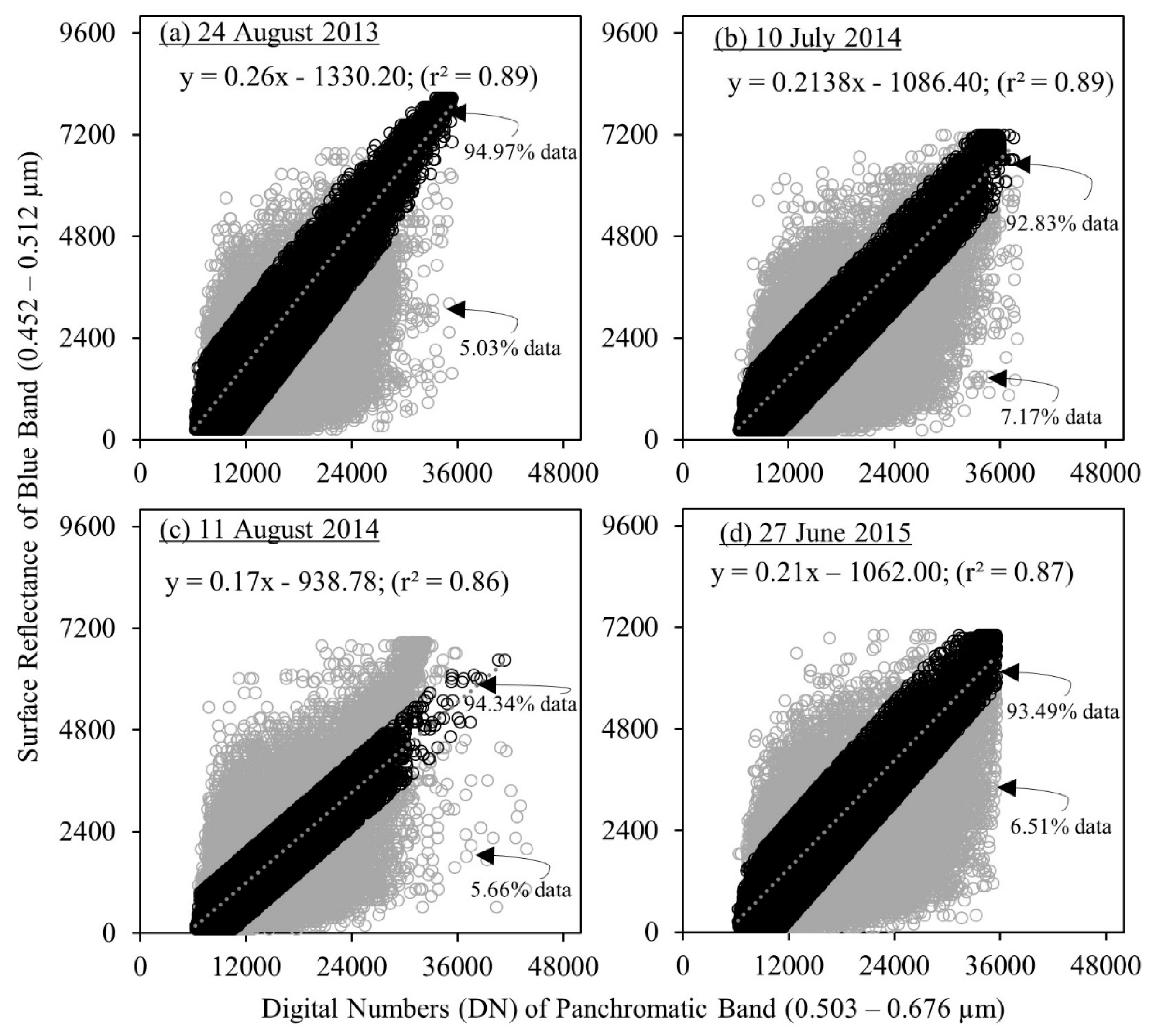
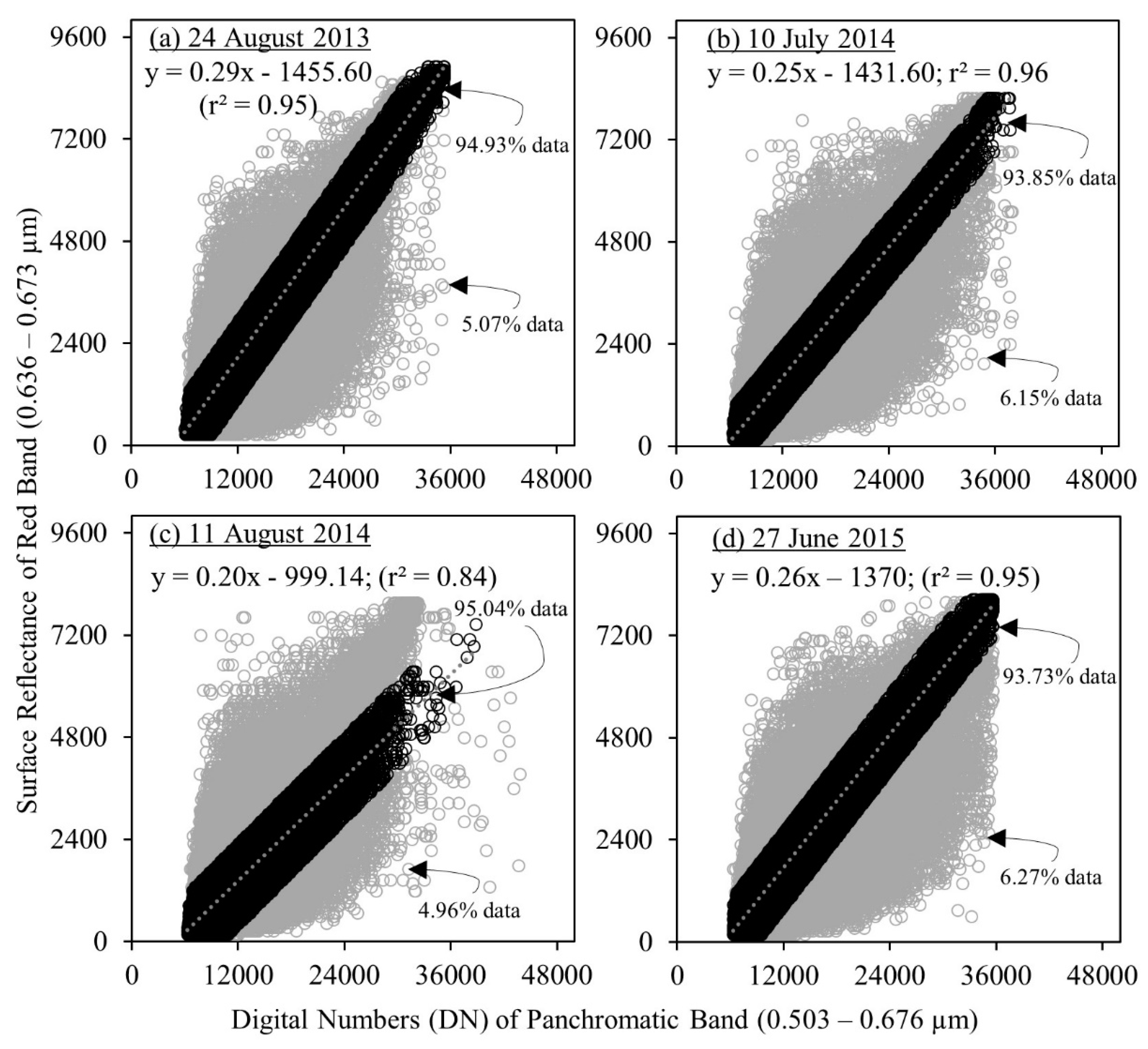
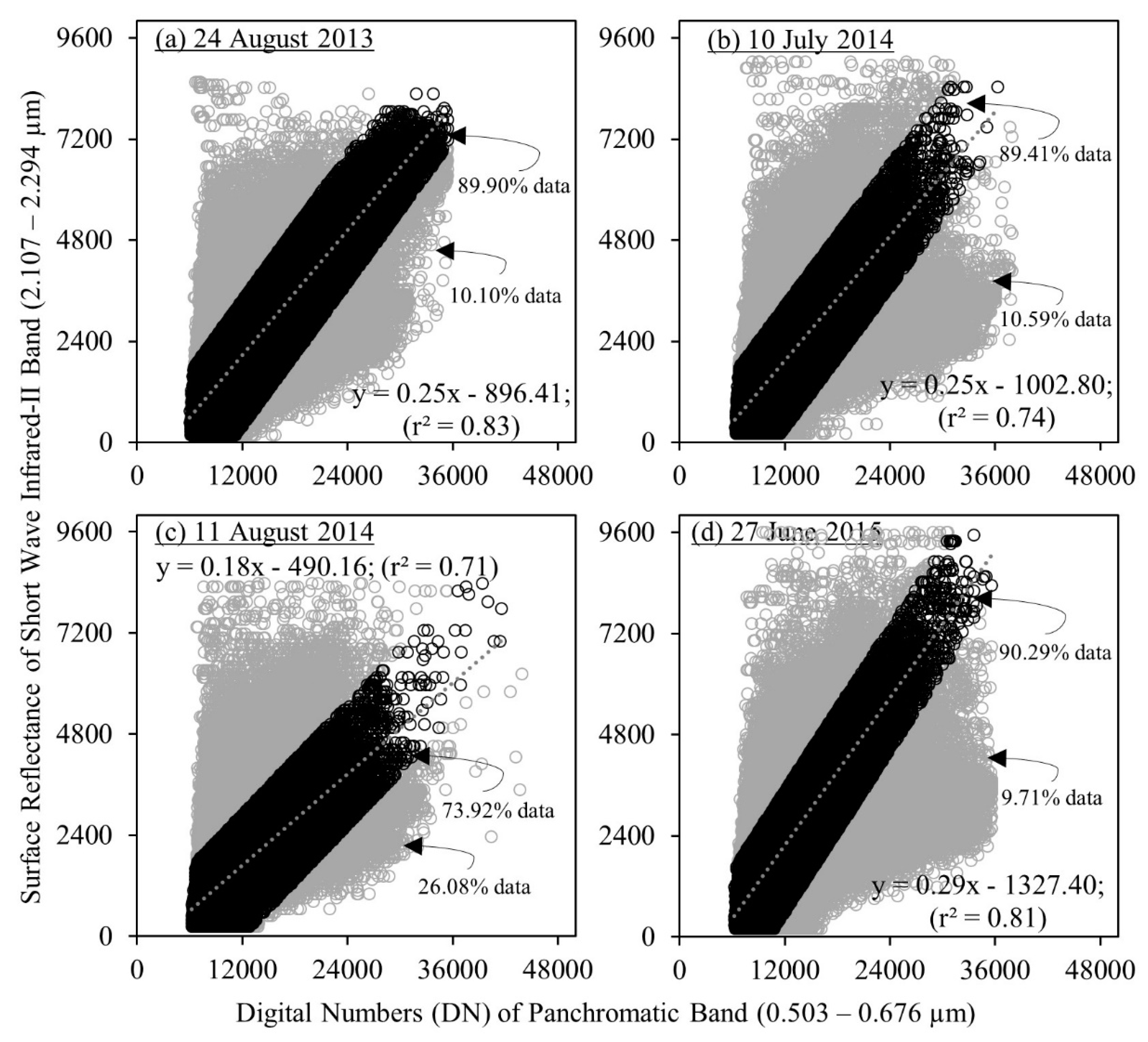
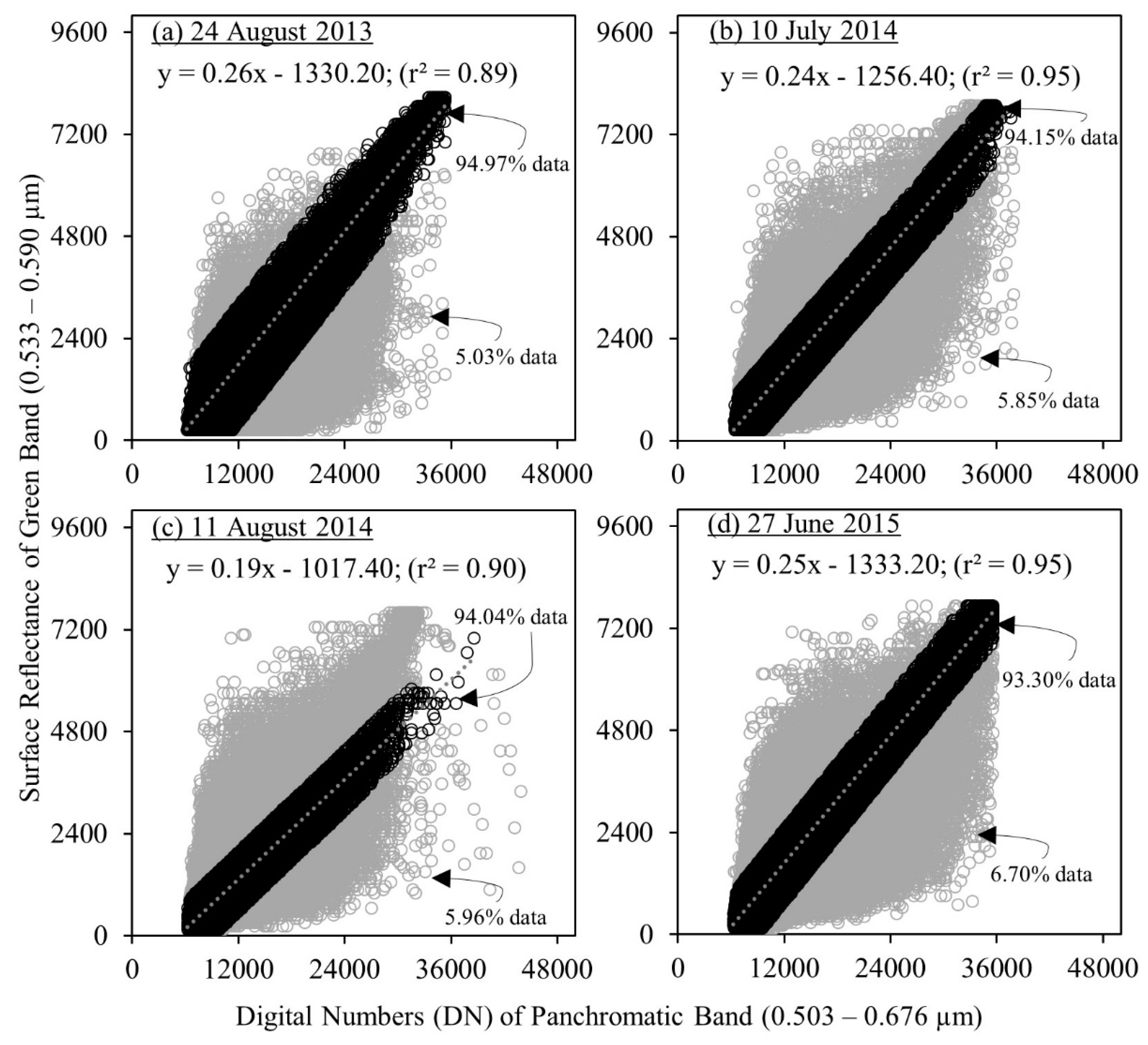
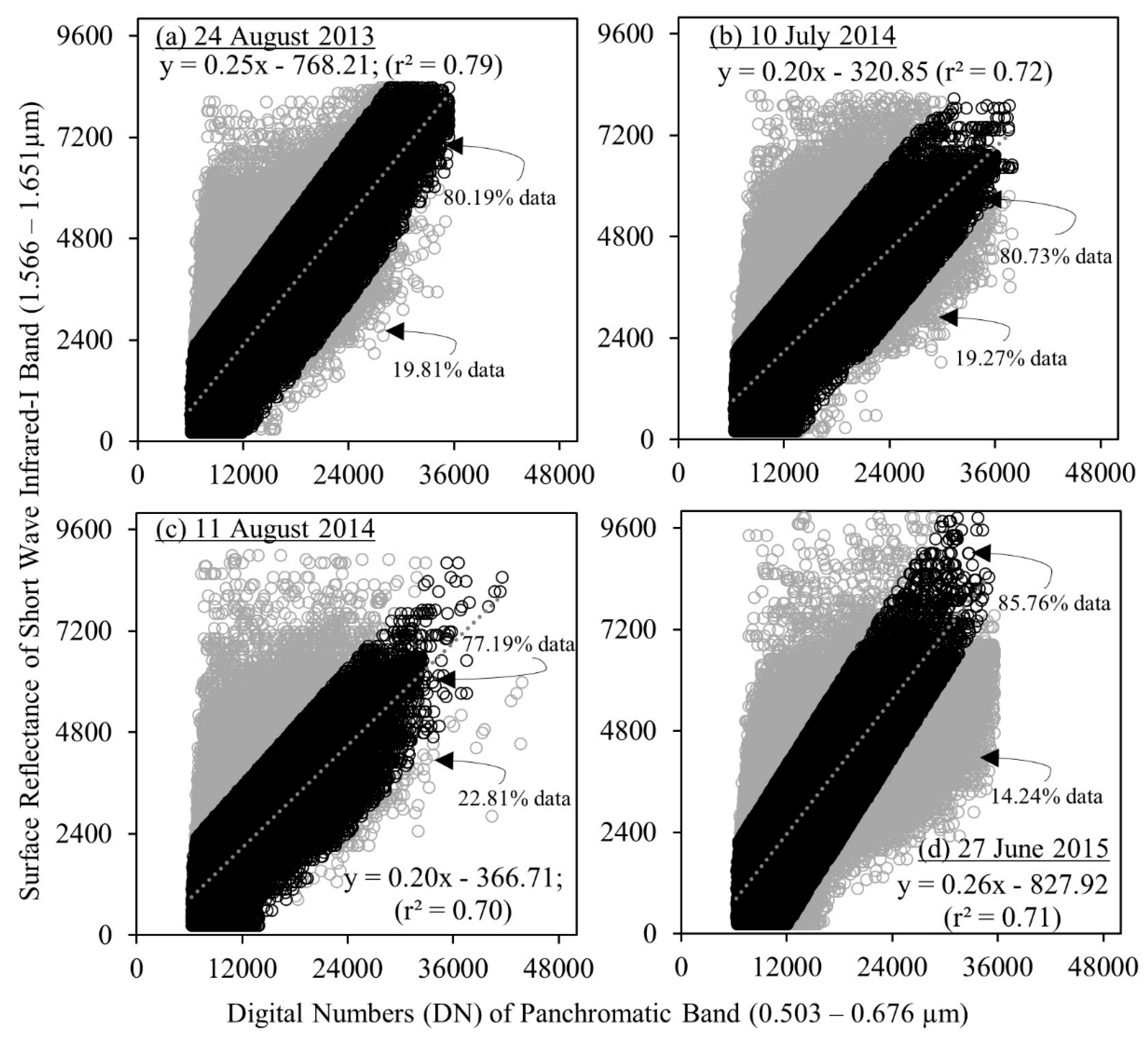
4.1. Comparing and Determining Relationships among PAN and MS Bands

Figure 3, Figure 4, Figure 5, Figure 6 and Figure 7 show the relationships between blue, green, red, SWIR-I, and SWIR-II (30 m spatial resolution) bands and PAN band (15 m spatial resolution) captured by the Landsat-8 OLI satellite. We plotted the data for four different days as can be seen inside the figures. All of the MS bands (except NIR) had strong relationships with the PAN band. For example, the r² values were found to be in the range: (i) 0.86–0.89 for blue band for approximately 93% of the data points; (ii) 0.89–0.95 for green band for approximately 93% of the data points; (iii) 0.84–0.96 for red band for approximately 94% of the data points; (iv) 0.71–0.79 for SWIR-I band for approximately 80% of the data points; and (v) 0.71–0.83 for SWIR-II band for approximately 74% of the data points.

It would be interesting to note that the relationships between PAN and MS bands of blue, green, and red were expected to be highly correlated. This would be due to the fact that the wavelengths of the PAN band (0.50–0.68 µm) overlapped with the visible bands, such as blue (0.45–0.51 µm), green (0.53–0.59 µm), and red (0.64–0.67 µm). Also, similar results have been reported in the literature. For example, when compared, researchers found that PAN and MS visible bands (i.e., blue, green, and red) of Landsat-8 OLI had a strong correlation with r² value ranging from 0.90 to 0.98 [36,37]. However, NIR band did not reveal a significant relationship with the PAN band. Among the four images acquired on different dates, NIR band exhibited relatively weaker relationship (i.e., r² value approximately 0.53). This would be expected as the spectral resolution of the NIR band (0.85–0.88 µm) had no overlap with the PAN band (0.50–0.68 µm). Literature also suggested that weaker relationships would exist between PAN and NIR bands of Landsat-8 OLI satellite images [1,2]. In addition, SWIR-I (1.57–1.65 µm), and SWIR-II (2.11–2.29 µm) bands did not have any overlap with PAN bands’ spectral resolution but had strong relationships in terms of r² values (i.e., approximately 0.70 to 0.90) (see Figure 6 and Figure 7). Note that similar results were observed in relevant literature, i.e., that SWIR bands had strong relationships with visible and PAN bands[37,38]. As a result, it was not surprising to see the outcomes once we found strong relationships among PAN and SWIR bands (i.e., SWIR-I and SWIR-II) in particular.

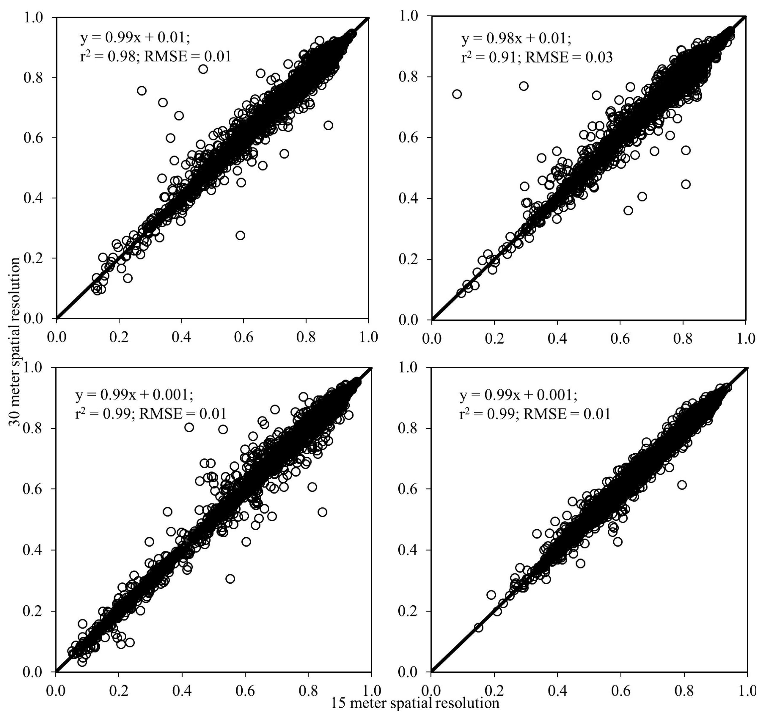
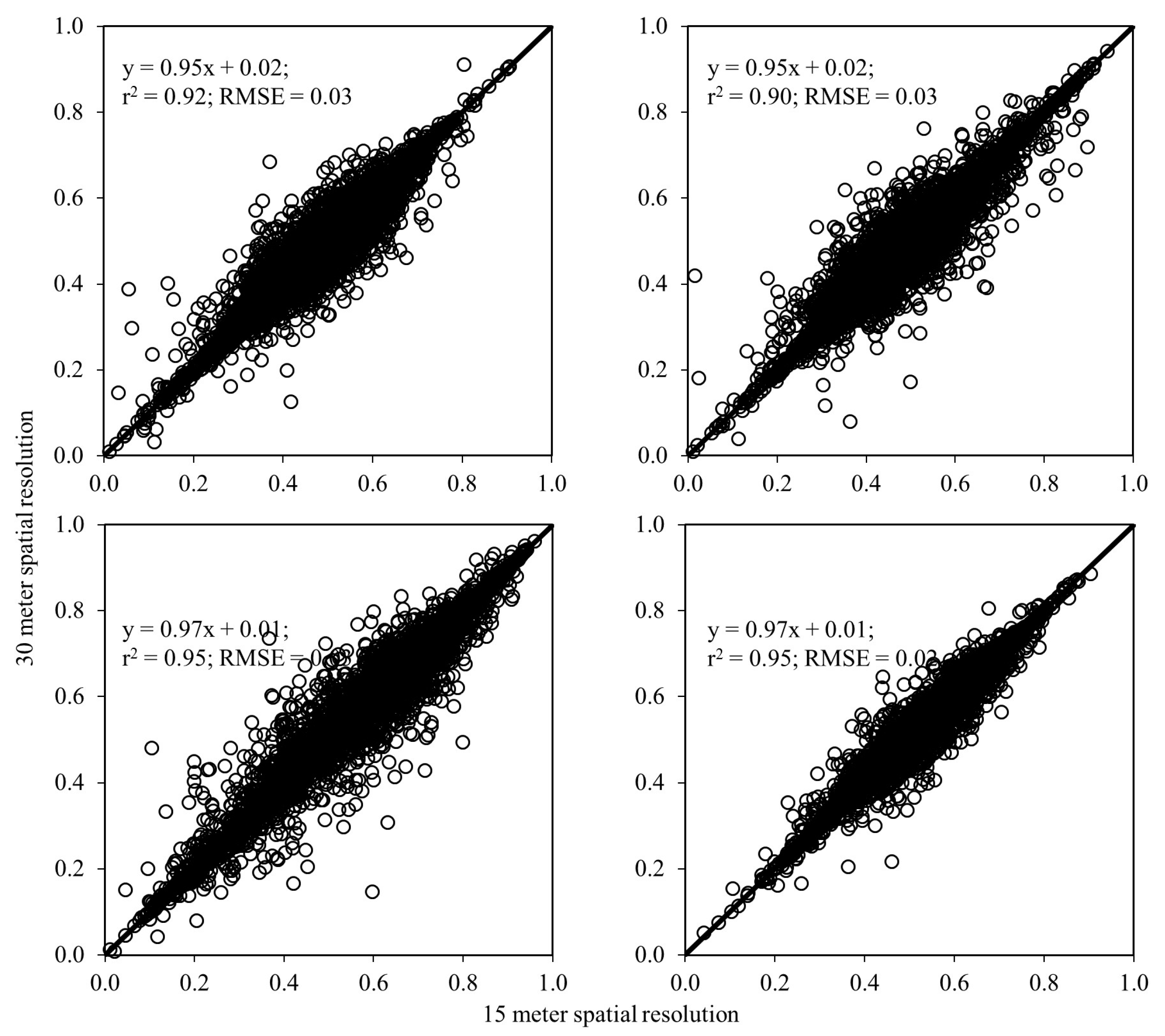
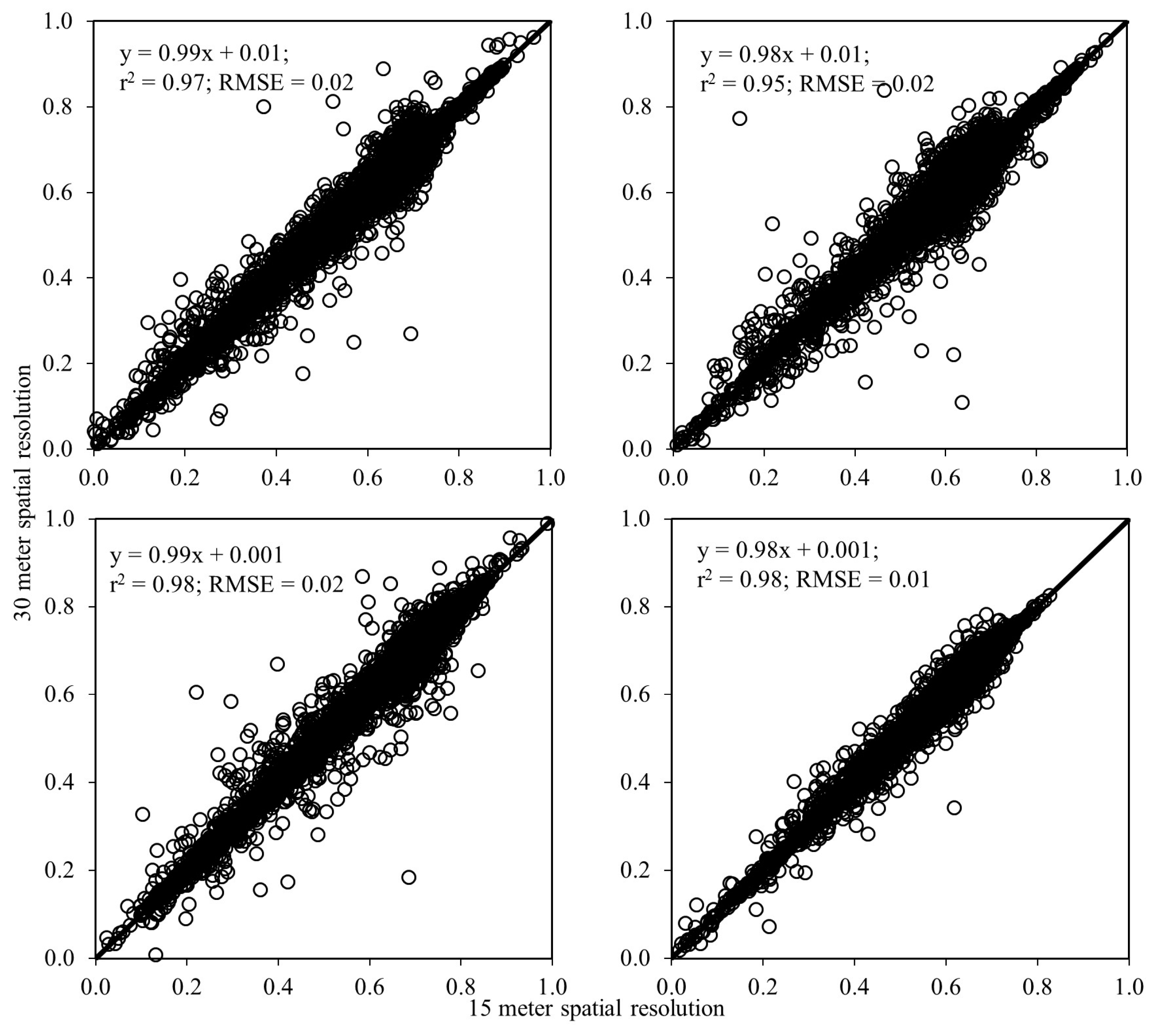
4.2. Generation of Vegetation and Canopy Moisture Contents and Their Validation

As we obtained significant relationships among MS and PAN bands, we decided to enhance the 30 m spatial resolution of MS bands to 15 m spatial resolution upon pan-sharpening (as outlined in Section 3). Once we enhanced the required MS bands with pan-sharpening procedures, we then calculated different vegetation indices (i.e., NDVI, EVI, and NDWI). For NDWI calculation, we performed the computation twice as, NDWI depends on SWIR-I and SWIR-II bands. Consequently, SWIR-I band was centered at 1.64 µm and SWIR-II band was centered at 2.20 µm (spectral resolution). For instance, our output results for NDWI were plotted twice. Figure 8, Figure 9, Figure 10 and Figure 11 show the results of computed NDVI, EVI, and NDWI indices. Relationships of validation were calculated by measuring the r², intercepts, slopes, and RMSE values, which were in the range: (i) 0.98–0.99, 0.01, 0.99, and 0.01, respectively, for NDVI; (ii) 0.90–0.95, 0.01–0.02, 0.95–0.97, and 0.02–0.03, respectively, for EVI; (iii) 0.95–0.98, 0.00–0.01, 0.98–0.99, and 0.01–0.02, respectively, for NDWI centered at 1.64 µm; and (iv) 0.98–1.00, 0.00, 0.99–1.00, and 0.00–0.02, respectively, for NDWI centered at 2.20 µm. Note that we were unable to compare our results with other studies as similar validation schemas were not found in the literature.

It is worthwhile to mention that earlier studies, in fact, emphasized calculating NDVI values at 15 m spatial resolution using pan-sharpening techniques (e.g., [2,25]). In Johnson [25], the author argued that the employment of the pan-sharpening algorithm adopted in this study as described in Section 3.2 would void the effect of the pan-sharpening goal. This would be the case as the formula of the NDVI calculation would remove the pan-sharpening component (i.e., Equation (2)), which was common for each of the considered variables. However, as we resampled the NIR band at 15 m, such limitation would not prevail in this study. Additionally, Gilbertson et al. [11] applied a pan-sharpening algorithm such as the synthetic variable ratio (SVR) method [1,11]. However, it was unclear whether they evaluated relationships between PAN and NIR bands of Landsat-8 OLI images, which was in fact the prerequisite of such actions. In this context, we evaluated such relationships and did not find significant correlations. As a result, such a pan-sharpening algorithm might not be applicable in the case of Landsat-8 OLI.

Finally, as the formula of all the considered indices, i.e., NDVI, EVI, and NDWI in this study (see Section 3.2 for details) had a common variable like NIR band, we resampled the NIR band instead of the pan-sharpened band for this particular spectral band of interest. Consequently, its application to calculate these above-mentioned indices at 15 m and their validation in comparison to the equivalent 30 m resolution provided a solid basis for adopting the proposed method of pan-sharpening.

4.3. Contributions

In the scope of this study, we implemented a pan-sharpening technique and its applicability to calculate several vegetation indices (i.e., EVI, NDVI, and SWIR). According to the best of our knowledge, several unique contributions and outcomes were identified, such as:

(i)

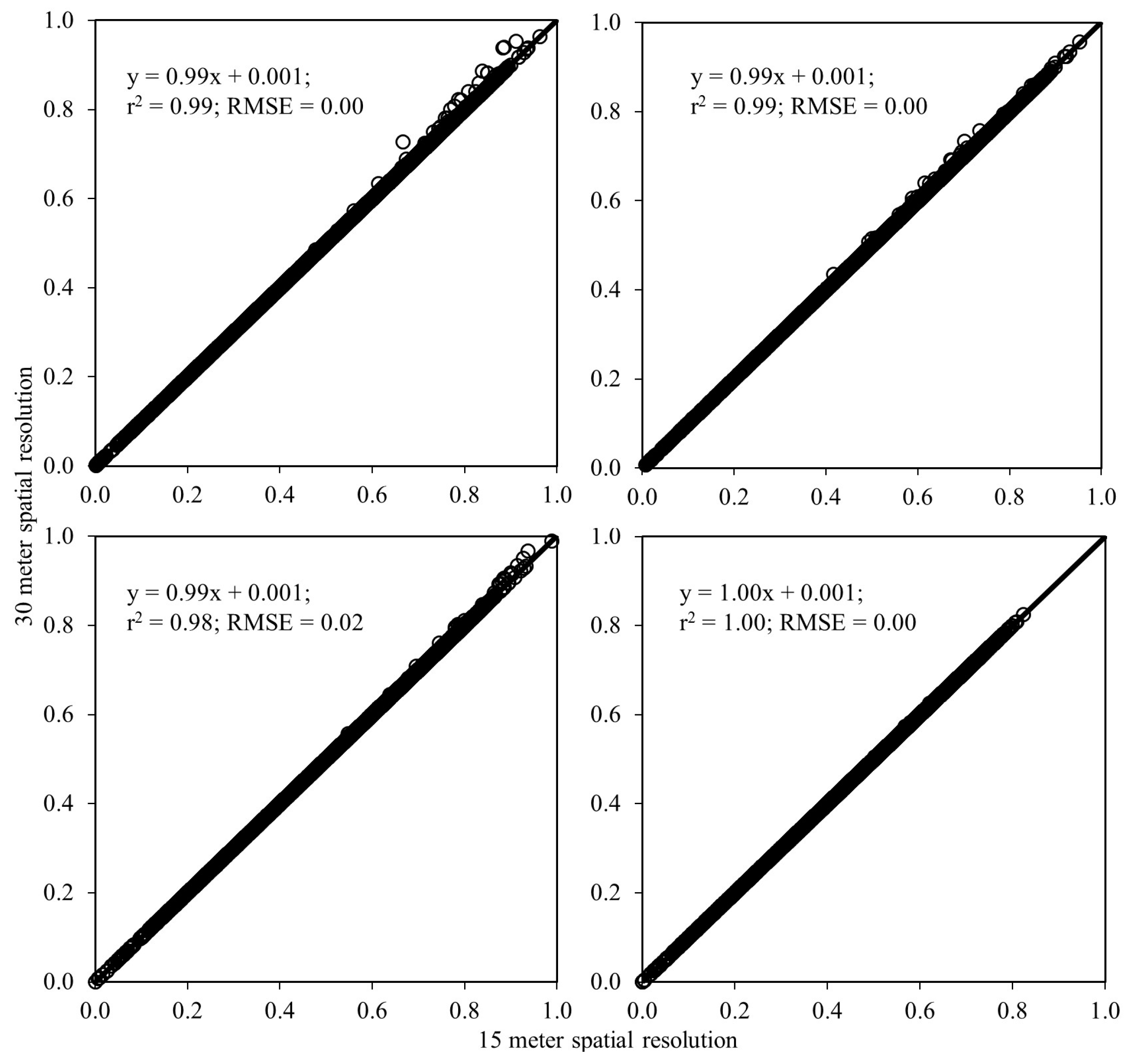
To our knowledge of the contemporary literature, comparison and/or correlation analysis between pan-sharpened NDVI, EVI, and NDWI products (@15 m spatial resolution) with their original spatial resolution (@30 m spatial resolution) had not been reported elsewhere;

(ii)

Landsat-8 OLI is a relatively newly launched satellite platform (operating since February 2013) [16]. The PAN band of this particular satellite differs from others. For example, the spectral resolution of the PAN band spans 0.503–0.676 µm with clearly no overlap with the blue, and NIR spectral bands. Note that other platforms, on the other hand, have overlapping spectral bands between PAN, and visible, and NIR bands. As a result, we assumed that the PAN band of the Landsat-8 should not be correlated with the NIR band, which, in fact, was proven in this study.

(iii)

Other studies [38,39,40,41] applied pan-sharpening over Landsat-8 data in order to derive NDVI-values alone. In these studies, we understood that they also pan-sharpened the NIR band, which might not be applicable to enhance vegetation indices as the relationship between the PAN and NIR band could not be significant. We thus mentioned in this study that NIR band would not yield better results if used in further enhancement of vegetation indices.

(iv)

We also calculated EVI (an indicator of vegetation canopy structure), and NDWI (an indicator of water stress of vegetation) using Landsat-8 OLI data and provided their validations.

5. Concluding Remarks

In this study, we proposed a simple protocol to generate NDVI, EVI, and NDWI at an enhanced spatial resolution of 15 m. In this case, we adopted a pan-sharpening method widely known as smoothing filter-based intensity modulation and enhanced the MS bands required to compute the above-mentioned indices of interest. Our results demonstrated strong relationships between each individual MS (blue, green, red, and SWIRs) and PAN band while comparing r² values (i.e., the values were ranged from 0.71 to 0.96) for the Landsat-8 OLI images. However, NIR band exhibited a weaker relationship which was not a surprising outcome as its wavelength was beyond the respective band width of the PAN band. Consequently, we generated the NDVI, EVI, and NDWI using the spatial resolution of MS bands enhanced to 15 m and resampled NIR band to 15 m. Then, we evaluated these indices with compare with the indices computed at 30 m spatial resolution for validation purposes. The results of the vegetation canopy moisture and greenness indices (i.e., NDVI, EVI, and NDWI) were then compared based on the values of r², slope, intercept, and RMSE. We found strong relationships among these values and argued that this method would help the pan-sharpening research community to obtain higher resolution Landsat-8 MS images for better results. Consequently, we suggest that before applying the pan-sharpening techniques, it is essential to calculate individual relationships of each MS band of interest with PAN band and then decide which specific band needs to be pan-sharpened. In addition, we believe that the use of the proposed technique will enhance the spectral and spatial resolution of Landsat-8 OLI MS bands which can be used for different environmental applications, such as land use change, vegetation indices calculation, and application in the field of agricultural research, etc. Finally, we also strongly suggest that the proposed schema should be thoroughly evaluated prior to implementation in other geographical locations.

References

1. Zhang, J. Multi-source remote sensing data fusion: Status and trends. Int. J. Image Data Fusion 2010, 1, 5–24. [Google Scholar] [CrossRef]
2. Vivone, G.; Alparone, L.; Chanussot, J.; Mura, M.D.; Garzelli, A.; Member, S.; Licciardi, G.A.; Restaino, R.; Wald, L. Pansharpening Algorithms. IEEE Trans. Geosci. Remote Sens. 2014, 53, 2565–2586. [Google Scholar] [CrossRef]
3. Laben, C.; Brower, B. Process for Enhancing the Spatial Resolution of Multispectral Imagery Using Pan-sharpening. U.S. Patent 6011875 A, 29 April 1998. [Google Scholar]
4. Jovanović, D.; Govedarica, M.; Sabo, F.; Važić, R.; Popović, D. Impact analysis of pansharpening Landsat ETM+, Landsat OLI, WorldView-2, and Ikonos images on vegetation indices. Procceedings of the Fourth International Conference on Remote Sensing and Geoinformation of the Environment, Paphos, Cyprus, 4 April 2016. [Google Scholar]
5. Bhatti, S.S.; Tripathi, N.K. Built-up area extraction using Landsat 8 OLI imagery. GIsci. Remote Sens. 2014, 51, 445–467. [Google Scholar] [CrossRef]
6. Bendib, A.; Dridi, H.; Kalla, M.I. Contribution of Landsat 8 data for the estimation of land surface temperature in Batna city, Eastern Algeria. Geocarto Int. 2016, 32, 1–11. [Google Scholar] [CrossRef]
7. Lwin, K.K.; Murayama, Y. Evaluation of land cover classification based on multispectral versus pansharpened landsat ETM+ imagery. GIsci. Remote Sens. 2013, 50, 458–472. [Google Scholar]
8. Wieland, M.; Pittore, M. Large-area settlement pattern recognition from Landsat-8 data. ISPRS J. Photogramm. Remote Sens. 2016, 119, 294–308. [Google Scholar] [CrossRef]
9. Ai, J.; Gao, W.; Gao, Z.; Shi, R.; Zhang, C.; Liu, C. Integrating pan-sharpening and classifier ensemble techniques to map an invasive plant ( Spartina alterniflora ) in an estuarine wetland using Landsat 8 imagery. J. Appl. Remote Sens. 2016. [Google Scholar] [CrossRef]
10. Johnson, B.A.; Scheyvens, H.; Shivakoti, B.R. An ensemble pansharpening approach for finer-scale mapping of sugarcane with Landsat 8 imagery. Int. J. Appl. Earth Obs. Geoinf. 2014, 33, 218–225. [Google Scholar] [CrossRef]
11. Gilbertson, J.K.; Kemp, J.; van Niekerk, A. Effect of pan-sharpening multi-temporal Landsat 8 imagery for crop type differentiation using different classification techniques. Comput. Electron. Agric. 2017, 134, 151–159. [Google Scholar] [CrossRef]
12. Hwang, T.; Song, C.; Bolstad, P.V.; Band, L.E. Downscaling real-time vegetation dynamics by fusing multi-temporal MODIS and Landsat NDVI in topographically complex terrain. Remote Sens. Environ. 2011, 115, 2499–2512. [Google Scholar] [CrossRef]
13. Howat, I.M.; Negrete, A.; Smith, B.E. The Greenland Ice Mapping Project (GIMP) land classification and surface elevation data sets. Cryosphere 2014, 8, 1509–1518. [Google Scholar] [CrossRef]
14. Roy, D.P.; Kovalskyy, V.; Zhang, H.K.; Vermote, E.F.; Yan, L.; Kumar, S.S.; Egorov, A. Characterization of Landsat-7 to Landsat-8 reflective wavelength and normalized difference vegetation index continuity. Remote Sens. Environ. 2016, 185, 57–70. [Google Scholar] [CrossRef]
15. Hassan, Q.K.; Bourque, C.P.; Meng, F.R.; Richards, W. Spatial mapping of growing degree days: An application of MODIS-based surface temperatures and enhanced vegetation index. J. Appl. Remote Sens. 2007. [Google Scholar] [CrossRef]
16. Acharya, T.D.; Yang, I.T. Exploring Landsat 8. Int. J. IT Eng. Appl. Sci. Res. 2015, 4, 4–10. [Google Scholar]
17. Aiazzi, B.; Baronti, S.; Lotti, F.; Selva, M. A Comparison Between Global and Context-Adaptive Pansharpening of Multispectral Images. IEEE Geosci. Remote Sens. Lett. 2009, 6, 302–306. [Google Scholar] [CrossRef]
18. Zhang, Y. Understanding Image Fusion. Photogramm. Eng. Remote Sens. 2004, 70, 657–661. [Google Scholar]
19. Karathanassi, V.; Kolokousis, P.; Ioannidou, S. A comparison study on fusion methods using evaluation indicators. Int. J. Remote Sens. 2007, 28, 2309–2341. [Google Scholar] [CrossRef]
20. Zhang, Y.; Hong, G. An IHS and wavelet integrated approach to improve pan-sharpening visual quality of natural colour IKONOS and QuickBird images. Inf. Fusion 2005, 6, 225–234. [Google Scholar] [CrossRef]
21. Zhang, Y.; Mishra, R. A review and comparison of commercially available pan-sharpening techniques for high resolution satellite image fusion. IEEE Geosci. Remote Sens. 2012. [Google Scholar] [CrossRef]
22. Du, Q.; Younan, N.H.; King, R.; Shah, V.P. On the performance evaluation of pan-sharpening techniques. IEEE Geosci. Remote Sens. Lett. 2007, 4, 518–522. [Google Scholar] [CrossRef]
23. Hassan, Q.K.; Bourque, C.P.A. Spatial enhancement of MODIS-based images of leaf area index: Application to the boreal forest region of northern Alberta, Canada. Remote Sens. 2010, 2, 278–289. [Google Scholar] [CrossRef]
24. Hazaymeh, K.; Hassan, Q.K. Fusion of MODIS and Landsat-8 surface temperature images: A new approach. PLoS ONE 2015, 10, e0117755. [Google Scholar] [CrossRef] [PubMed]
25. Johnson, B. Effects of pansharpening on vegetation indices. ISPRS Int. J. Geoinf. 2014, 3, 507–522. [Google Scholar] [CrossRef]
26. Pushparaj, J.; Hegde, A.V. Comparison of various pan-sharpening methods using Quickbird-2 and Landsat-8 imagery. Arab. J. Geosci. 2017. [Google Scholar] [CrossRef]
27. Maglione, P.; Parente, C.; Vallario, A. Pan-sharpening worldview-2: IHS, brovey and zhang methods in comparison. Int. J. Eng. Technol. 2016, 8, 673–679. [Google Scholar]
28. Liu, J.G. Smoothing filter-based intensity modulation: A spectral preserve image fusion technique for improving spatial details. Int. J. Remote Sens. 2010, 21, 3461–3472. [Google Scholar] [CrossRef]
29. Zhang, Y.; Mishra, R.K. From UNB PanSharp to Fuze Go—The success behind the pan-sharpening algorithm. Int. J. Image Data Fusion 2014, 5, 39–53. [Google Scholar] [CrossRef]
30. Yusuf, Y.; Sri Sumantyo, J.T.; Kuze, H. Spectral information analysis of image fusion data for remote sensing applications. Geocarto Int. 2013, 28, 291–310. [Google Scholar] [CrossRef]
31. Yuhendra; Alimuddin, I.; Sumantyo, J.T.S.; Kuze, H. Assessment of pan-sharpening methods applied to image fusion of remotely sensed multi-band data. Int. J. Appl. Earth Obs. Geoinf. 2012, 18, 165–175. [Google Scholar] [CrossRef]
32. Zhu, X.X.; Bamler, R. A sparse image fusion algorithm with application to pan-sharpening. IEEE Trans. Geosci. Remote Sens. 2013, 51, 2827–2836. [Google Scholar] [CrossRef]
33. Natural Regions and Subregions of Alberta. Available online: https://www.albertaparks.ca/media/6256258/natural-regions-subregions-of-alberta-a-framework-for-albertas-parks-booklet.pdf (accessed on 4 April 2017).
34. Rahaman, K.R.; Hassan, Q.K. Quantification of local warming trend: A remote sensing-based approach. PLoS ONE 2017, 12, e0169423. [Google Scholar] [CrossRef] [PubMed]
35. Hassan, Q.K.; Bourque, C.P.; Meng, F.R. Application of Landsat-7 ETM+ and MODIS products in mapping seasonal accumulation of growing degree days at an enhanced resolution. J. Appl. Remote Sens. 2007, 1. [Google Scholar] [CrossRef]
36. Jing, L.; Cheng, Q. Two improvement schemes of PAN modulation fusion methods for spectral distortion minimization. Int. J. Remote Sens. 2009, 30, 2119–2131. [Google Scholar] [CrossRef]
37. Zhang, H.K.; Roy, D.P. Computationally inexpensive Landsat 8 Operational Land Imager (OLI) pansharpening. Remote Sens. 2016, 8, 180. [Google Scholar] [CrossRef]
38. Kaufman, Y.J.; Tanré, D.; Remer, L.A.; Vermote, E.F.; Chu, A.; Holben, B.N. Operational remote sensing of tropospheric aerosol over land from EOS moderate resolution imaging spectroradiometer. J. Geophys. Res. 1997, 102, 17051–17067. [Google Scholar] [CrossRef]
39. Castanho, A.D.; Prinn, R.; Martins, V.; Herold, M.; Ichoku, C.; Molina, L.T. Analysis of Visible/SWIR surface reflectance ratios for aerosol retrievals from satellite in Mexico City urban area. Atmos. Chem. Phys. 2007, 7, 5467–5477. [Google Scholar] [CrossRef]
40. Zhang, Y. Problem of fusion of commercial high-resolution satellite as well as Landsat 7 image and initial solutions. Int. Arch. Photogramm. Remote Sens. Spat. Inf. Sci. 2002, 34, 587–592. [Google Scholar]
41. Rodriguez-Galiano, V.; Pardo-Iguzquiza, E.; Sanchez-Castillo, M.; Chica-Olmoa, M.; Chica-Rivas, M. Downscaling Landsat 7 ETM+ thermal imagery using land surface temperature and NDVI images. Int. J. Appl. Earth Obs. Geoinf. 2012, 18, 515–527. [Google Scholar] [CrossRef]
Figure 1. Depiction of the study area using a Landsat-8 OLI image acquired on 11 August 2014 (panel (b)) in the Western Canadian context (panel (a)). The Landsat image is a true color composite consisting of the spectral bands of blue, green, and red at 30 m spatial resolution. Note that the dark green color in panel (b) represents vegetation cover, the light green color represents agricultural land, and the black color represents water bodies. In addition, the grey color represents built up areas and other land areas except vegetation and agriculture.
Ijgi 06 00168 g001
Figure 2. Schematic diagram of the methods illustrating the pan-sharpening process and its use in calculating vegetation greenness and canopy moisture indices.
Ijgi 06 00168 g002
Figure 3. Relationships between surface reflectance of blue band and PAN band. The black dots are the data points considered for analysis while the grey dots are considered as outliers. The small dotted line represents the linear regression line.
Ijgi 06 00168 g003
Figure 4. Relationships between surface reflectance of green band and PAN band. The black dots are the data points considered for analysis while the grey dots are considered as outliers. The small dotted line represents the linear regression line.
Ijgi 06 00168 g004
Figure 5. Relationships between surface reflectance of red band and PAN band. The black dots are the data points considered for analysis while the grey dots are considered as outliers. The small dotted line represents the linear regression line.
Ijgi 06 00168 g005
Figure 6. Relationships between surface reflectance of SWIR-I band and PAN band. The black dots are the data points considered for analysis while the grey dots are considered as outliers. The small dotted line represents the linear regression line.
Ijgi 06 00168 g006
Figure 7. Relationships between surface reflectance of SWIR-II band and PAN band. The black dots are the data points considered for analysis while the grey dots are considered as outliers. The small dotted line represents the linear regression line.
Ijgi 06 00168 g007
Figure 8. Relationships between NDVI derived at 15 m and 30 m spatial resolution.
Ijgi 06 00168 g008
Figure 9. Relationships between EVI derived at 15 m and 30 m spatial resolution.
Ijgi 06 00168 g009
Figure 10. Relationships between NDWI@1.64 µm derived at 15 m and 30 m spatial resolution.
Ijgi 06 00168 g010
Figure 11. Relationships between NDWI@2.20 µm derived at 15 m and 30 m spatial resolution.
Ijgi 06 00168 g011