
Generalized Aggregation of Sparse Coded Multi-Spectra for Satellite Scene Classification


1
Graduate School of Science and Technology for Innovation, Yamaguchi University, 1677-1 Yoshida, Yamaguchi City, Yamaguchi 753-8511, Japan
2
College of Information Science and Engineering, Ritsumeikan University, 1-1-1 Nojihigashi, Kusatsu 525-8577, Japan
*
Author to whom correspondence should be addressed.
†
Current address: Yamaguchi University, 1677-1 Yoshida, Yamaguchi City, Yamaguchi 753-8511, Japan
ISPRS Int. J. Geo-Inf. 2017, 6(6), 175; https://0-doi-org.brum.beds.ac.uk/10.3390/ijgi6060175
Submission received: 25 April 2017
/
Revised: 10 June 2017
/
Accepted: 13 June 2017
/
Published: 16 June 2017
Abstract
:Satellite scene classification is challenging because of the high variability inherent in satellite data. Although rapid progress in remote sensing techniques has been witnessed in recent years, the resolution of the available satellite images remains limited compared with the general images acquired using a common camera. On the other hand, a satellite image usually has a greater number of spectral bands than a general image, thereby permitting the multi-spectral analysis of different land materials and promoting low-resolution satellite scene recognition. This study advocates multi-spectral analysis and explores the middle-level statistics of spectral information for satellite scene representation instead of using spatial analysis. This approach is widely utilized in general image and natural scene classification and achieved promising recognition performance for different applications. The proposed multi-spectral analysis firstly learns the multi-spectral prototypes (codebook) for representing any pixel-wise spectral data, and then, based on the learned codebook, a sparse coded spectral vector can be obtained with machine learning techniques. Furthermore, in order to combine the set of coded spectral vectors in a satellite scene image, we propose a hybrid aggregation (pooling) approach, instead of conventional averaging and max pooling, which includes the benefits of the two existing methods, but avoids extremely noisy coded values. Experiments on three satellite datasets validated that the performance of our proposed approach is very impressive compared with the state-of-the-art methods for satellite scene classification.
1. Introduction
The rapid progress in remote sensing imaging techniques over the past decade has produced an explosive amount of remote sensing (RS) satellite images with different spatial resolutions and spectral coverage. This allows us to potentially study the ground surface of the Earth in greater detail. However, it remains extremely challenging to extract useful information from the large number of diverse and unstructured raw satellite images for specific purposes, such as land resource management and urban planning [1,2,3,4]. Understanding the land on Earth using satellite images generally requires the extraction of a small sub-region of RS images for analysis and for exploring the semantic category. The fundamental procedure of classifying satellite images into semantic categories firstly involves extracting the effective feature for image representation and then constructing a classification model by using manually-annotated labels and the corresponding satellite images. The success of the bag-of-visual-words (BOW) model [5,6,7] and its extensions for general object and natural scene classification has resulted in the widespread application of these models for solving the semantic category classification problem in the remote sensing community. The BOW model was originally developed for text analysis and was then adapted to represent images by the frequency of ”visual words” that are generally learned from the pre-extracted local features from images by a clustering method (K-means) [5]. In order to reduce the reconstruction error led by approximating a local feature with only one ”visual word” in K-means, several variant coding methods such as sparse coding (Sc), linear locality-constrained coordinate (LLC) [8,9,10,11] and the Gaussian mixture model (GMM) [12,13,14,15] have been explored in the BOW model for improving the reconstruction accuracy of local features, and some researchers further endeavored to integrate the spatial relationships of the local features. On the other hand, local features such as SIFT [16], which is handcrafted and designed as a gradient-weighted orientation histogram, are generally utilized and remain untouched in terms of their strong effect on the performance of these BOW-based methods [17,18,19]. Therefore, some researchers investigated the local feature learning procedure automatically from a large number of unlabeled RS images via unsupervised learning techniques instead of using the handcrafted local feature extraction [20,21,22], thereby improving the classification performance to some extent. Recently, deep learning frameworks have witnessed significant success in general object and natural scene understanding [23,24,25] and have also been applied to remote sensing image classification [26,27,28,29,30]. These framework perform impressively compared with the traditional BOW model. All of the above-mentioned algorithms firstly explore the spatial structure for providing the local features, which is important for local structure analysis in high-definition general images, such as those in which a single pixel covers several centimeters or millimeters. However, the available satellite images are usually acquired at a ground sampling distance of several meters, e.g., 30 m for Landsat 8 and 1 m even for high-definition satellite images from the National Agriculture Imagery Program (NAIP) dataset [31]. Thus, the spatial resolution of a satellite image is much lower than that of a general image, and the spatial analysis of nearby pixels, which often belong to different categories in a satellite image, may not be suitable. Recently, Zhong et al. [32] proposed an agile convolution neural network (CNN) architecture, named SatCNN, for high-spatial resolution RS image scene classification, which used smaller kernel sizes for building the effective CNN architecture and validated promising performance.
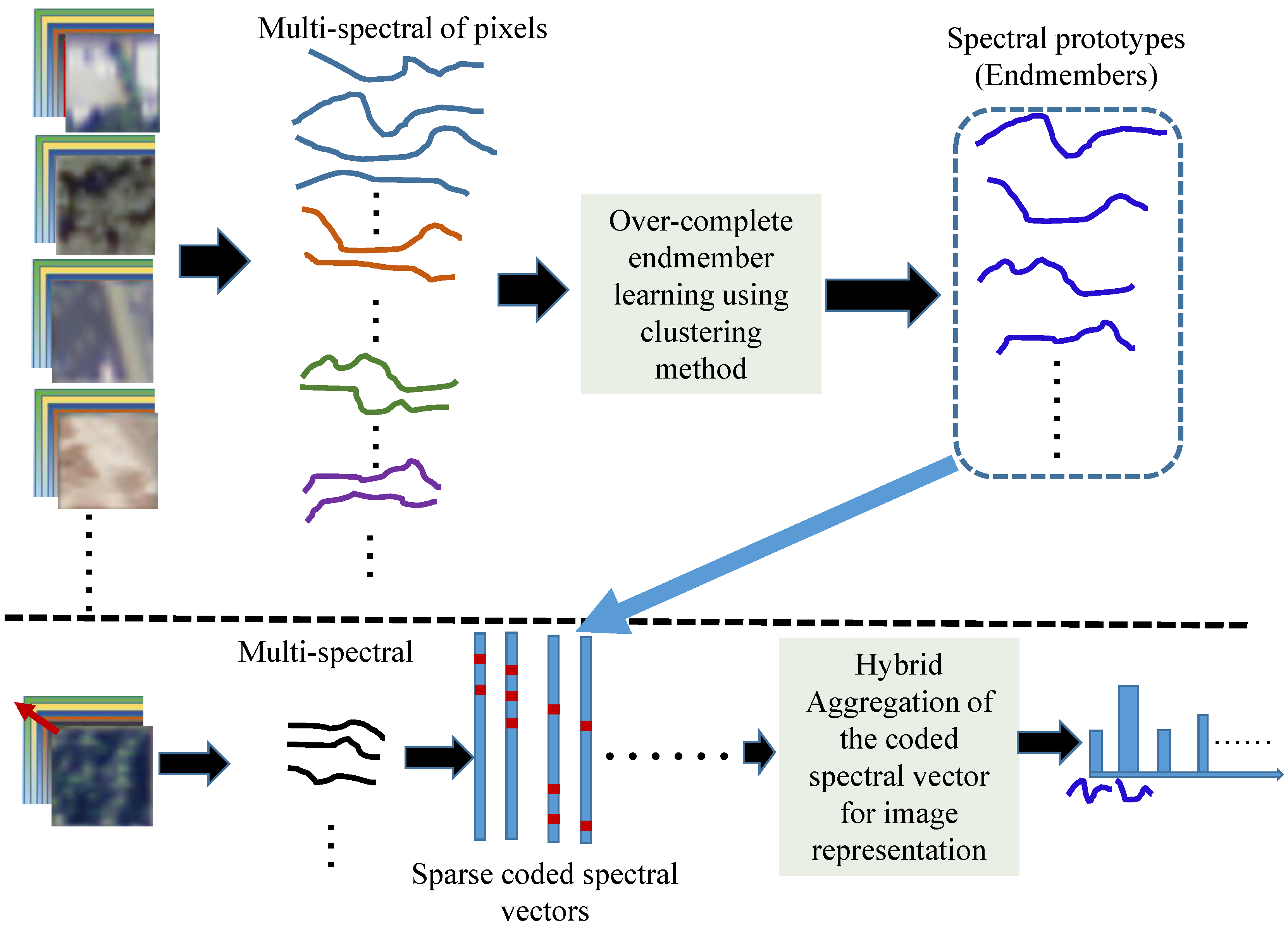
On the other hand, despite its low spatial resolution, a satellite image is usually acquired in multiple spectral bands (also known as hyper-spectral data), which is expected for pixel-wise land cover investigation even with mixing pixels. It is labor intensive to concentrate on the traditional mixing pixel recovery problem (known as the unmixing model) [33,34,35]. This model can obtain material composition fraction maps and a set of spectra of pure materials (also known as endmembers) and has achieved acceptable pure pixel recovery results. These pixel-wise methods assume that the input images contain pure endmembers and that they can process the image with mixed pixels of several or dozens of endmembers. This study aims to classify a small sub-region of the satellite image into a semantic category by considering that a pixel spectrum in an explored sub-region is a supposition of several spectral prototypes (possible endmembers). At the same time, because of the large variety of multi-spectral pixels even for the same material due to environmental changes, we generate an over-complete spectral prototype set (dictionary or codebook), which means that the number of prototypes is larger than the number of spectral bands. It also takes into consideration the variety of multi-spectral pixels for the same material, whereas most optimization methods for simplex (endmember) identification [36,37,38,39] in an unmixing model generally only obtain a sub-complete prototype set, thereby possibly ignoring some detailed spectral structures for representation. Therefore, based on the learned over-complete spectral codebook, any pixel spectrum can be well reconstructed by a linear combination of only several spectral prototypes to produce a sparse coded vector. Furthermore, deciding how to aggregate the sparse coded spectral vector for the sub-region representation is a critical step for affecting the final recognition performance. In the conventional BOW model and its extensions with the spatially-analyzed local features, the coded vectors in an image are generally aggregated with an average or max pooling strategy. The average pooling simply takes the mean value of the coded coefficients corresponding to a learned visual word, which is specially utilized accompanied with hard assignment (i.e., representing any local feature using only one visual word), whereas max pooling takes the maximum value of all coded coefficients in an image or region corresponding to a learned visual word (atom), which is applied accompanied with soft-assignment or sparse coding approaches. The max pooling strategy accompanied with sparse coding approaches achieved promising performance in the classification and detection of different objects, which means that only exploiting the highest activation status of the local description prototype (possibly a distinct local structure in an object with spatial analysis) is effective. However, the max pooling strategy only retains the strongest activated pattern and would completely ignore the frequency: an important signature for identifying different types of images of the activated patterns. In addition, because of the low spatial resolution of satellite images, the exploration of spatial analysis and pixel-wise spectral analysis to provide the composition fraction of any spectral prototype would be unsuitable. We aim to obtain the statistical fractions of each spectral prototype to represent the explored sub-region, whereas max-pooling unavoidably ignores almost all of the coded spectral coefficients, while average pooling would take the coded spectral coefficients of some outliers to form the final representation. Therefore, this study proposes a hybrid aggregation (pooling) strategy of the sparse coded spectral vectors by integrating not only the maximum magnitude, but also the response magnitude of the relatively large coded coefficients of a specific spectral prototype, a process named K-support pooling. This proposed hybrid pooling strategy combines the popularly-applied average and max pooling methods and, rather than awfully emphasizing the maximum activation, preferring a group of activations in the explored region instead. The proposed satellite image representation framework is shown in Figure 1, where the top row is for over-complete spectral prototype set learning, and the bottom row manifests the sparse coding of any pixel spectral and the hybrid pooling strategy of all coded spectral vectors in a sub-region to form the discriminated feature.
Because of the low spatial resolution of satellite images, this study explores the spectral analysis method instead of spatial analysis, which is widely used in general object and natural scene recognition. The main contributions of our work are two-fold: (1) unlike the spectral analysis in the unmixing model, which usually only obtains the sub-complete basis (the number of the bases is fewer than the number of spectral bands) via simplex identification approaches, we investigate the over-complete dictionary for more accurate reconstruction of any pixel spectrum and obtain the reconstruction coefficients by using a sparse coding technique; (2) we generate the final representation of a satellite image from all coded sparse spectral vectors, for which we propose a generalized aggregation strategy. This strategy not only integrates the maximum magnitude, but also the response magnitude of the relatively large coded coefficients of a specific spectral prototype instead of employing the conventional max and average pooling approaches.
This paper is organized as follows. Section 2 describes related work including the BOW model based on spatial analysis and the multi-spectral unmixing problem by assuming a limited number of bases (endmembers) and the corresponding abundance for each spectral pixel. The proposed strategy, which entails sparse coding for multi-spectral representation of pixels, is introduced in Section 3 together with a generalized aggregation approach for coded spectral vectors. The experimental results and discussions are provided in Section 4. Finally, the concluding remarks are presented in Section 5.
2. Related Work
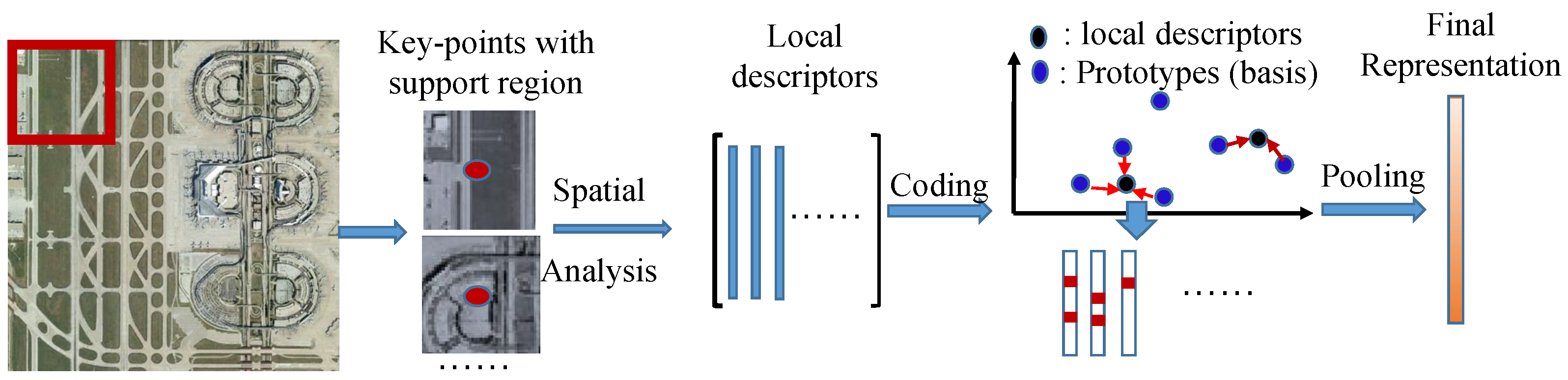
Considerable research efforts are being devoted to understanding satellite images. Among the approaches researchers have developed, the bag-of-visual-words (BOW) model [5,6,7] and its extensions have been widely applied to land-use scene classification. In general, this type of classification considers large-scale categories (with coverage of tens or hundreds of meters in one direction) such as airports, farmland, ports and parks. A flowchart of the BOW model is shown in Figure 2 and includes the following three main steps: (1) local descriptor extraction, which concentrates to explore the spatial relation of nearby pixel and ignores or separately analyzes the intensity variation of different colors (spectral bands) by using methods such as SIFT [16] and SURF [40]; (2) a coding procedure, which approximates a local feature using a linear combination of pre-defined or learned bases (codebook), and transforms each local feature into a more discriminated coefficient vector; (3) a pooling step, which aggregate all of the coded coefficient vectors in the region of interest into the final representation of this region via a max or average pooling strategy. The local descriptor in the BOW model for most applications usually remains untouched as SIFT and SURF, of which the design is handcrafted for exploring the local distinctive structure of the target objects. The local descriptor, which is most generally used, namely SIFT, needs to roughly and uniformly quantize the gradient direction between the nearby pixels into several orientation bins; however, this would cause the loss of some subtle structures and affect the final image representation ability. Therefore, some researchers investigated the local feature extraction procedure by automatically learning from a large number of unlabeled images with unsupervised learning techniques instead of using the handcrafted local feature extraction [20,21,22] and improved the classification performance to some extent. However, all of the above-mentioned algorithms mainly concentrate on spatial analysis to explore the distinctive local structure of general objects and take less consideration of the color (spectra) information, an approach that would be unsuitable for satellite scene classification as a result of its low spatial resolution. Recently, developments in deep convolutional networks have witnessed great success in different image classification applications, including applications involving the use of remote sensing images; however, these methods still focus on convoluting a spatial supported region into local feature maps. Because of the presence of multiple available spectral bands in satellite images, this study proposes to investigate the pixel spectral band and validate the feasibility and effectiveness for satellite scene classification.
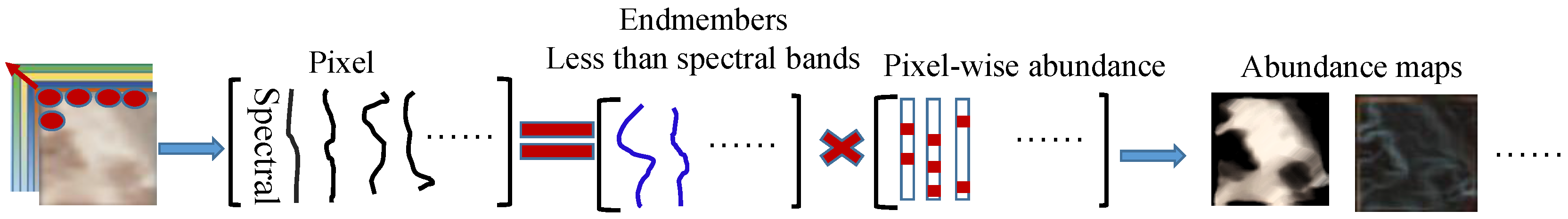
On the other hand, the existence of multiple spectral bands (also known as hyper-spectral data) in satellite images has promoted many researchers to propose pixel-wise land cover investigation to enable the variety of mixed pixels, known as an unmixing model [33,34,35], to be processed. The purpose of the unmixing model is to decompose the raw satellite images, composed of mixed pixels, into several material composition fraction maps and the corresponding set of pure spectral materials (also known as endmembers). The flowchart representing this procedure is shown in Figure 3. Given a multi-spectral satellite image with size (where B denotes the number of spectral bands and N and M denote the height and width of the satellite image, respectively), where the pixels may cover several types of land materials due to the low spatial resolution, we first re-arrange the image in the form of a matrix with a pixel-wise spectral column vector (size: ). The spectral vector of the i-th pixel is assumed to be a linear combination of several endmembers (basis) with the composition fraction as the weighted coefficients: , where is a set of spectral column vectors (K) representing the existing endmembers (land materials) in the processed satellite image. Considering the physical phenomenon of the spectral image, the elements in the endmember spectra and the fraction magnitude of the pixel abundance are non-negative, and the abundance vector for each pixel is summed to one. Then, the matrix formula for all pixels in a satellite image of interest can be formed as follows:
Much work has been devoted to concentrating the endmember determination, which is usually considered as a simplex identification problem [36,37,38,39]. However, the unmixing procedure is investigated in an image-wise approach, and the endmember and the abundance have been optimized independently for different images, which leads to completely different endmembers for different images. Furthermore, only a sub-complete set of the simplex (the number of simplexes are fewer than the number of spectral bands) can be obtained in the optimization. This study aims to learn a common set of bases (endmembers) for different sub-regions of satellite images, and an over-complete dictionary is preferred to take into consideration the variety of pixels in the same material and possible outliers in the target application. In the next section, we describe our proposed strategy in detail.
3. Generalized Aggregation of Sparse Coded Multi-Spectra
The low spatial resolution of satellite images, for example a ground sampling distance of each pixel in Landsat 8 images, has led us to focusing on the multiple spectral bands of a single pixel for statistical analysis. Let be the set of D-dimensional spectral vectors of all pixels extracted from a satellite image, i.e., . Our goal is first to code the spectral vector to a more discriminated coefficient vector based on a set of common bases (codebook). Given a codebook with K entries, , different coding schemes can transform each spectrum into a K-dimensional coded coefficient vector to generate the final image representation. Next, we provide the detail of the codebook (an over-complete basis) learning and coding methods.
3.1. Codebook Learning and Spectral Coding Approaches
The most widely-applied codebook learning and vector coding strategy in general object recognition applications is the vector quantization (VQ) method. However, because this strategy approximates any input vector with only one learned base, it possibly leads to a large reconstruction error. Therefore, several efforts have been made to approximate an input vector using a linear combination of several bases such as sparse coding (SC) and locality-constrained linear coding (LLC). These methods have been proven to perform impressively in different general object and natural scene classifications. As mentioned in [11], the smoothness of coded coefficient vectors is more important than the sparse constraint. This means the coded coefficient vector should be similar if the inputs are similar. Therefore, this study focuses on locality-constrained sparse coding for multi-spectral analysis.
Vector quantization: given training samples , the codebook learning procedure with VQ solves the following constrained least-squares fitting problem:
where is the set of codes for . The cardinality constraint means that there will be only one non-zero element in each code , corresponding to the quantization of . The non-negative constraint , and the sum-to-one constraint means that the summation of the coded weight for is one. The codebook can be learned from the prepared training samples, which are the spectral vectors of all pixels from a large number of satellite images, by the expectation maximization (EM) strategy. The detail of the algorithm of the VQ implementation in Equation (2) is shown in Algorithm 1. In the VQ method, the codebook vectors can be freely assigned as any larger number than the dimension of the input spectral vector , which forms an over-complete dictionary. After learning the codebook using the training spectral samples, it is fixed for coding the multi-spectral vectors of all pixels. The VQ approach can obtain the sparsest representation vector for an input vector (only one non-zero value), which means that it only approximates any input vector with one selected base from the codebook and thus leads to large reconstruction error. Therefore, several researchers proposed the use of sparse coding for vector coding, which can adaptively select several bases to approximate the input vector and thus reduce the reconstruction error. Sparse coding has been proven to perform more effectively in different applications.
Locality-constrained sparse coding: In terms of local coordinate coding, Wang et al. [11] claimed that locality is more important than sparsity, which not only leads to sparse representation, but also retains the smoothness between the transformed representation space and the input space. Therefore, this study incorporates a locality constraint instead of the pure sparsity constraint in Equation (3). This approach can simultaneously result in sparse representation, known as the locality-constraint sparse coding (LcSC), which is applied for codebook learning and spectral coding with the following criteria:
where the first term is the reconstruction error for the used samples and the second term is the constraint of locality and implicit sparsity. ⊙ denotes the element-wise multiplication, and the constraint allows the shift-invariant codes. is the locality controller for supplying different freedom of each basis vector proportional to its similarity to the input descriptor . We define the controller vector as the following:
where is used for adjusting the rate of weight decay for the locality controller. The locality controller vector imposes very large weight on the coded coefficients of the basis vectors that have no similarity (large distance) to the input vector, and in the results, the coefficients corresponding to the basis vectors that are not similar would be extremely small or zero. Therefore, the resulting coded vector for any input would be sparse and smooth between the coded space and the input space as a consequence of only using similar basis vectors. The detail implementation of the LcSC method in Equation (3) is shown in Algorithm 2. in Algorithm 2 is initialized with the VQ method.
| Algorithm 1 Codebook learning of VQ method in Equation (2). | |
| Input: | |
| Output: | |
| Initialization: Randomly take K samples from for initializing : . | |
| 2: | for do |
| for do | |
| 4: | Calculate the Euclidean distance between and , and assign |
| to cluster if , | |
| end for | |
| 6: | Recalculate with the assigned samples to the k-th cluster |
| end for | |
| 8: | Repeat the above Steps 2–7 until the predefined iteration is arrived or the change of the codebook becomes small enough in two consecutive iterations. |
| Algorithm 2 Codebook learning of LcSC method in Equation (3). | |
| Input: , , , | |
| Output: | |
| 1: | Initialization:. |
| 2: | for do |
| 3: | for do |
| 4: | Calculate the control element between and using Equation (4), |
| 5: | end for |
| 6: | Normalize : ; |
| 7: | Calculate the temporary coded vector with the fixed codebook using Equation (3), |
| 8: | Refine the coded vector via selecting the atoms with the larger coded coefficients only: |
| , , and | |
| , . | |
| 9: | Update : , where and , |
| 10: | Project back to : |
| 11: | end for |
3.2. Generalized Aggregation Approach
Given a satellite image sub-region, the multi-spectral vectors having the same number of pixels can be generated and thus produce the same number of coded coefficient vectors using coding approaches. The approach selected to aggregate the obtained coefficient vectors to form the final representation of the investigated sub-region plays an essential role in determining the recognition results of this region. As we know, the widely-used pooling methods for aggregating the encoded coefficient vectors in the traditional BOW model and its extension versions are average and max strategies. Average pooling aggregates all of the weighted coefficients, which are the coded coefficients of a pre-learned word in the BOW model, in a defined region by taking the average value, whereas max pooling aggregates these by taking the maximum value. In the vision community, the max pooling in combination with popularly-used coding methods such as SC and soft assignment manifests promising performance in a variety of image classification applications. However, the max-pooling strategy only retains the strongest activated pattern (the learned visual word) and would completely ignore the frequency of the activated patterns (visual words). This frequency counting the number of local descriptors, which are similar to the learned visual words, is also an important signature for identifying different types of images. Therefore, this study proposes a hybrid aggregation (pooling) strategy of the sparse coded spectral vectors by integrating not only the maximum magnitude, but also the response magnitude of the relatively large coded coefficients of a specific spectral prototype, termed K-support pooling. This proposed hybrid pooling strategy combines the popularly used average- and max-pooling methods and can avoid emphasizing the maximum activation; instead, it prefers using a group of activations in the explored region.
Let us denote the coded coefficient weight of the k-th codebook vector for the n-th multi-spectra in a satellite image as . We aim to aggregate all of the coded weights of the k-th codebook vector in the image to obtain the overall weight indication as the following:
where denotes the pooled coded weight of of the k-th codebook vector in the image . We can design different transformation functions f for aggregating the set of activations into a indicating value. The simplest pooling method simply averages the coded weights of all input vectors in this processed image formulated as:
The average-pooling strategy is generally used in the original BOW model, which assigns a local feature only to a nearest word and thus produces coded coefficients with a value of either one or zero. It eventually creates the representative histogram of the learned words for an image. Motivated by the visual biological study, the maximum activation would be more related to the human cortex response than the average activation and can provide translation-invariant visual representation. Therefore, the max pooling strategy has been widely used accompanied with SC and soft assignment coding strategies in the BOW model. The max-pooling can be formulated as:
Max pooling takes the maximum coded weights of all input vectors in an images as the overall activation degree and then completely ignores how many inputs are possibly activated. This study proposes a hybrid aggregation (pooling) strategy of the sparse coded spectral vectors by integrating not only the maximum magnitude, but also the response magnitude of the relatively large coded coefficients of a specific spectral prototype. The resulting integration is named K-support pooling. The proposed generalized aggregation approach firstly sorts the coefficient weight of the k-th codebook vector of all inputs from large to small values in a processed image as:
and then only retains the first L larger coefficient weights. The final activation degree of the processed prototype is calculated by averaging the retained L-values, which is the mean of the selected L-support locations (pixels), named as K-support pooling. It is formulated as the following:
For each codebook vector, we repeat the above procedure and produce the activation degrees of all codebook vectors in a processed image. Finally, the L aggregated coefficient weights can be obtained for representing the processed image.
3.3. SVM Classifier for Satellite Images
In this study, we use support vector machine (SVM) as the classifier for satellite images. Support vector machines are supervised learning models with a set of training examples and their corresponding labels. With the training samples, an SVM algorithm builds a classification model that assigns new examples to one category or the other. More formally, a support vector machine constructs a hyperplane or set of hyperplanes in a high-dimensional space, which can be used for classification, regression and so on. The generally used SVM can be divided into two categories: linear and nonlinear versions. In this study, we apply linear SVM as the classifier of satellite images. With the extracted features (described in the above subsections) from the training images and the corresponding class labels, we constructs multi-class SVM classification model using one-to-all strategy and then predict the class label of the extracted feature from an unknown-label image.
4. Experiments
4.1. Datasets
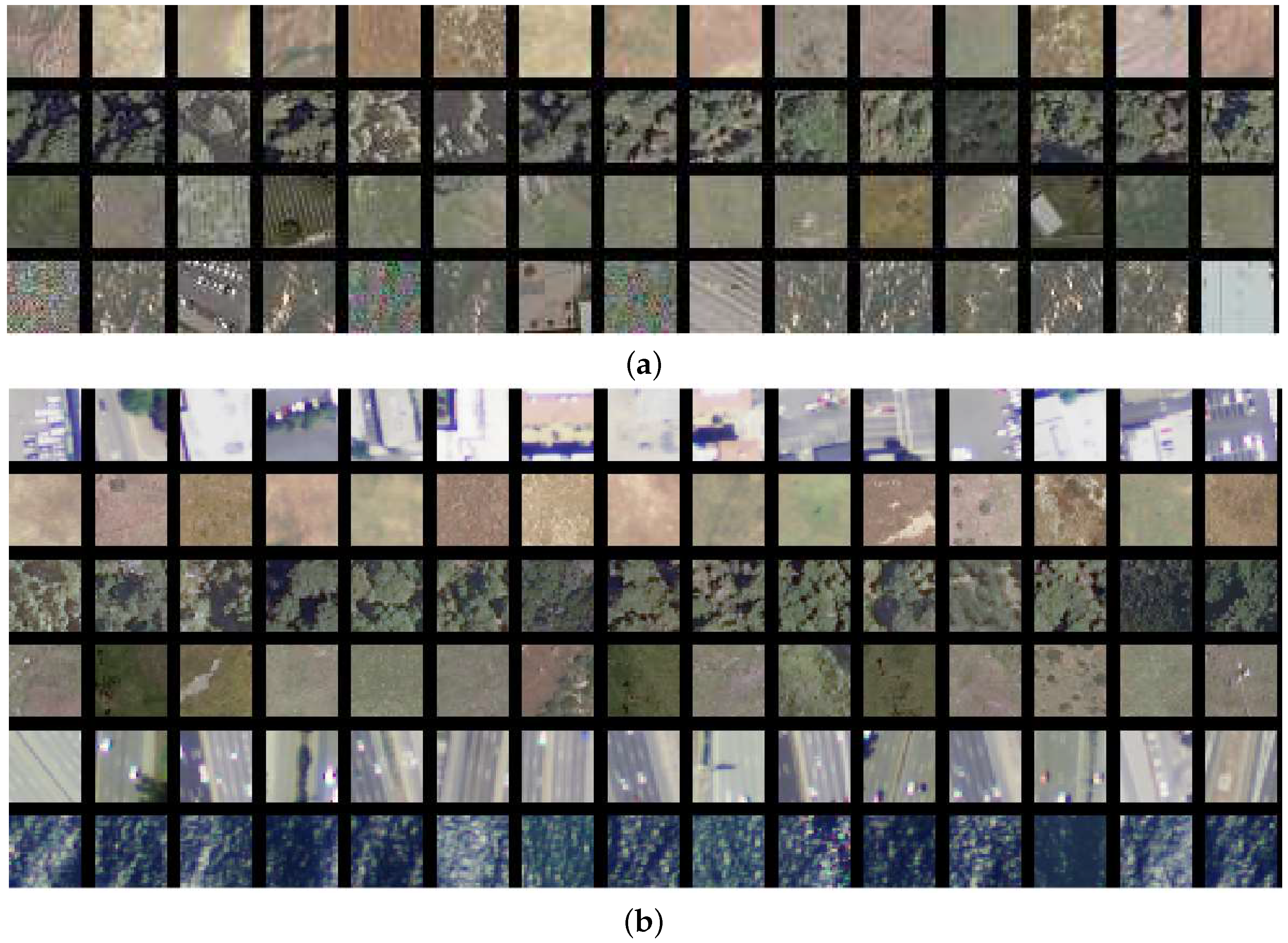
We evaluate our proposed image representation strategy with the generalized aggregated vector of the sparse coded multi-spectra on a benchmark database of satellite imagery classification, the DeepSat dataset [29], and a Megasolar dataset [41]. The DeepSat dataset includes two subsets: SAT-4 and SAT-6, which were released in [29]. The images in this dataset are from the National Agriculture Imagery Program (NAIP), and each is cropped to a sub-region. There are four spectral channels, red, green, blue and near-infrared (NIR), which means each pixel can be represented as a four-dimensional vector. SAT-4 consists of a total of 500,000 images, of which 400,000 images were chosen for training and the remaining 100,000 were used as the testing dataset. Four broad land cover classes were considered: barren land, trees, grassland and a class that includes all land cover classes other than the three. SAT-6 consists of a total of 405,000 images with 324,000 images as the training and 81,000 as the testing dataset. This dataset includes six land cover classes: barren land, trees, grassland, roads, buildings and water bodies. The sample images representing different classes from SAT-4 and SAT-6 are shown in Figure 4a,b, respectively. Several studies have been carried out to recognize the land cover classes in the SAT-4 and SAT-6 datasets. There are two state-of-the-art studies of land use recognition on SAT-4 and SAT-6. Motivated by the recent success of the deep learning framework, Basu et al. proposed a DeepSat architecture, which firstly extracted different statistical features from the input images and then fed them into a deep brief network for classification. Compared with several deep learning architectures, i.e., deep belief network (DBN), deep convolutional network (DCN) and stacked denoising autoencoder (SDE) via the raw image as the input, the proposed DeepSat could achieve a much more accurate recognition performance. In addition, Ma et al. proposed integrating the inception module from GoogleNet in the deep convolutional neural network to overcome the multi-scale variance of the satellite images and achieved some improvement in terms of the recognition performance for the SAT-4 and SAT-6 datasets. We compare the recognition performance using our proposed spectral analysis framework and the state-of-the-art based on deep learning techniques in the experimental results subsection.
In addition, we also give the classification performance with our proposed method on a Megasolar dataset [41], which was collected from 20 satellite images taken in Japan, 2015, by Landsat 8. The used image have 7 channels corresponding to different wavelengths, where half correspond to the non-visible infra-red spectrum, and their resolution is roughly 30 m per pixel. The satellite images are divided into cells; more than 20% of the pixels covered by a power plant are considered as positive samples, while those without a single pixel belonging to a power plant are treated as negative samples. There are 300 training positive samples augmenting to 4851 by rotation transformation and 2,247,428 training negative samples. The positive samples in validation and test subset are 126, and the negative samples are more than 860,000. In our experiments, we exploited the augmented 4851 positive samples and randomly selected 4851 negative samples from training subset for training, and the 126 positive samples in validation and test subsets and randomly selected 3000 negative samples are for the test.
4.2. Spectral Analysis
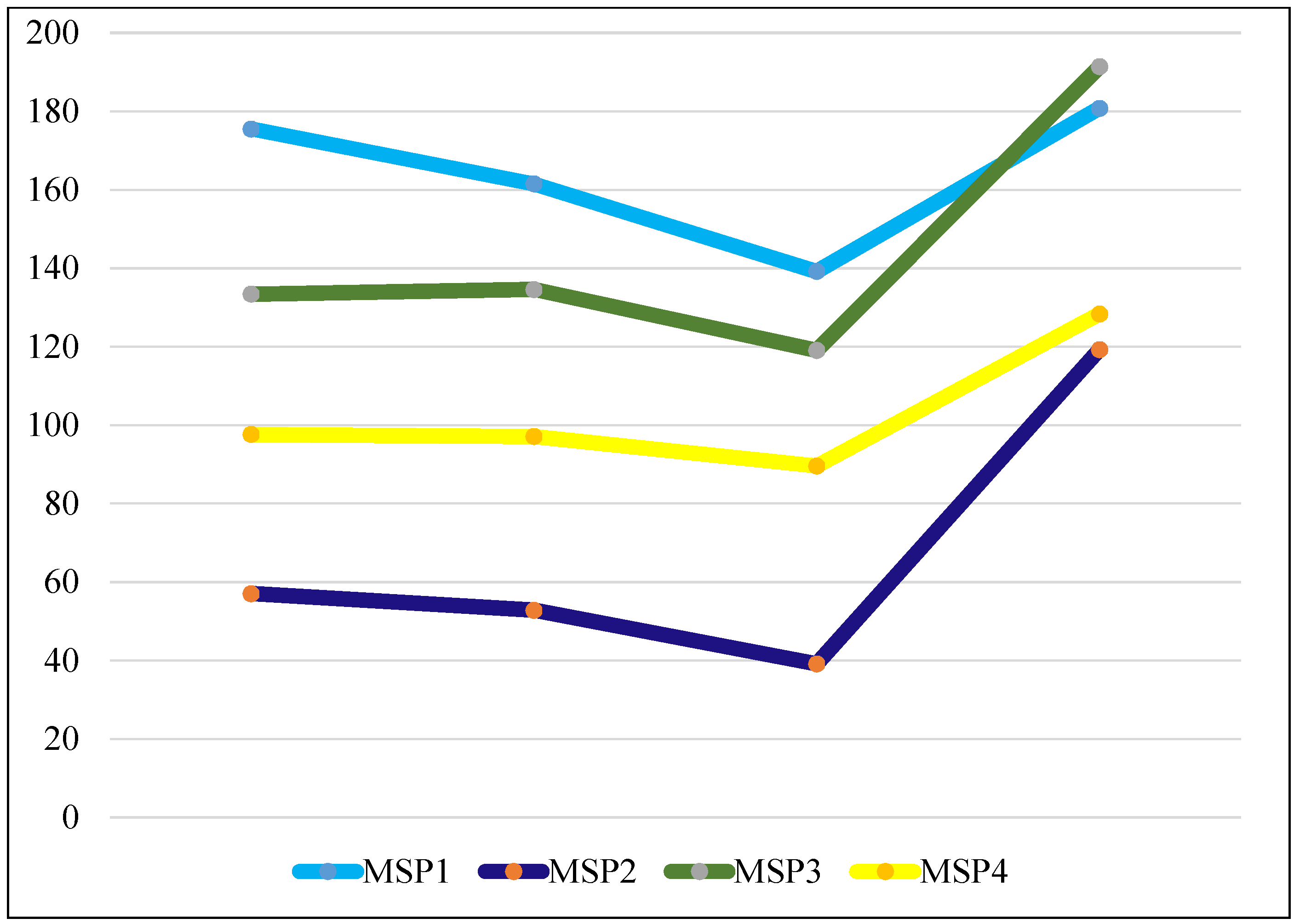
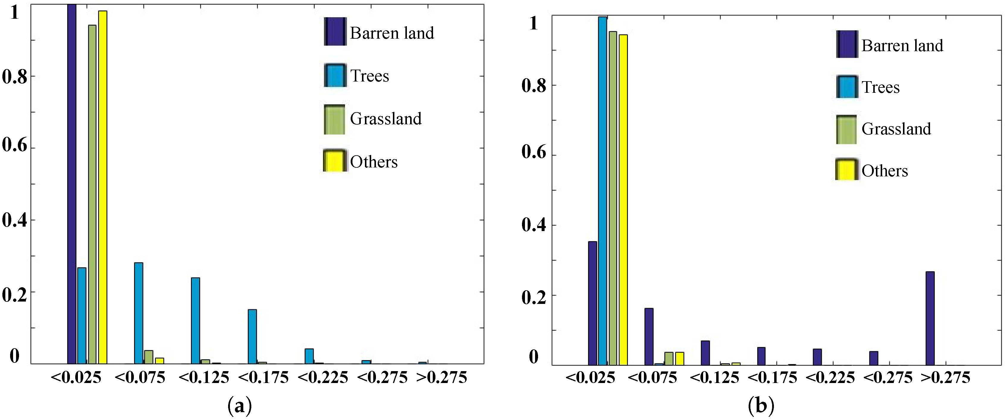
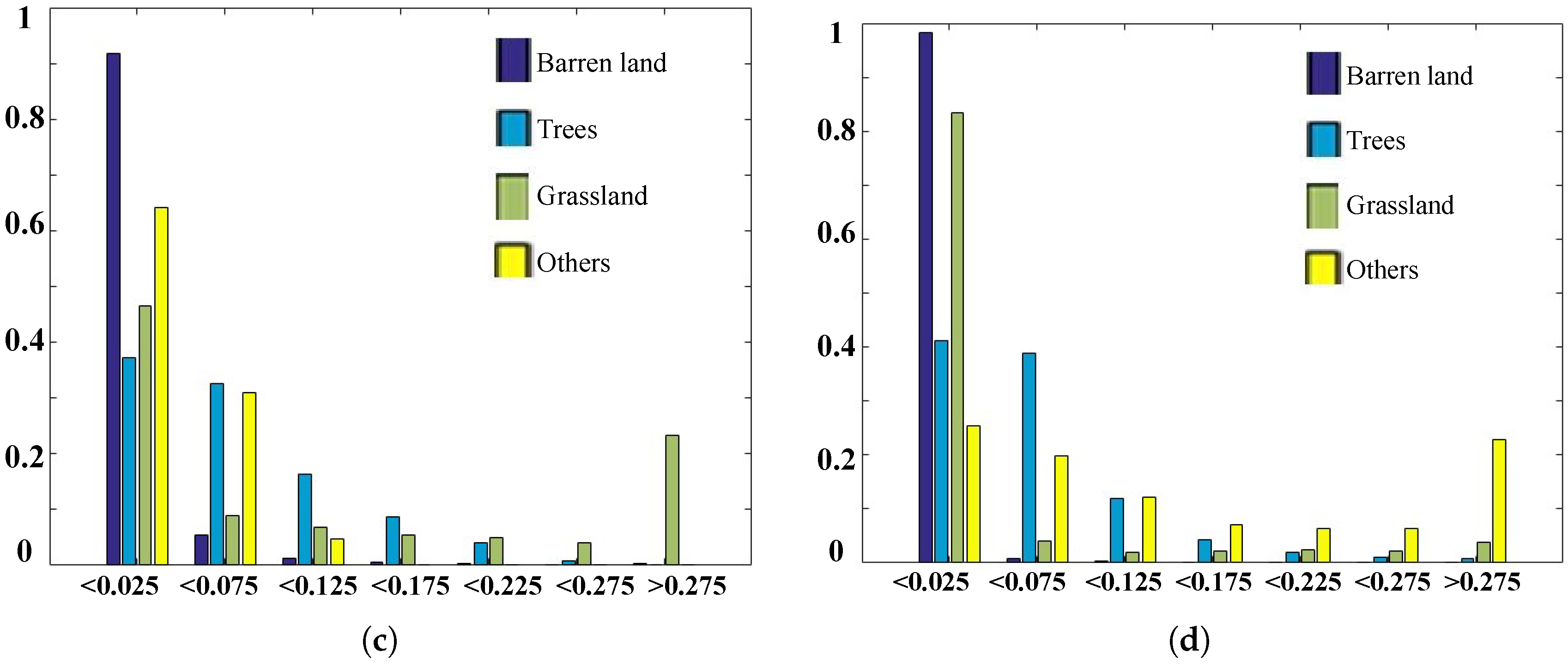
In our proposed strategy, we first need to learn the multi-spectral prototypes. In the implementation, we randomly select 1000 images from each class of the training dataset (SAT-4 and SAT-6, respectively) and generate the pixel-wise multi-spectral vectors from all of the selected images for learning the multi-spectral prototypes. Based on the introduced codebook learning approach, the K multi-spectral prototypes can be obtained. Figure 5 shows four multi-spectral prototypes of the learned codebook (32) using the SAT-4 dataset. Figure 6a–d indicates the image statistics of the coefficient weights corresponding to the considered prototypes (multi-spectral Prototype 1 (MSP1), MSP2, MSP3 and MSP4 from Figure 6a–d), where the horizontal and vertical axes denote the aggregated weight width of the four multi-spectral prototypes and image frequencies of each land use class in the defined weight regions, respectively. From Figure 6a, we can see that the second class (steel blue bar: trees) contains a greater number of images with large weights, whereas more than 90% of the images from the other three classes exhibit very small weights (less than 0.025). This means that the multi-spectral prototype, MSP1 in Figure 5, mainly represents the spectral data of trees material. Figure 6b confirms that the first class (midnight blue bar: barren land) contains more images with large weights, whereas more than 90% of the images from the other three classes manifest very small weights (less than 0.025). This means that the multi-spectral prototype, MSP2 in Figure 5, mainly represents the spectral data of barren land material. From Figure 6c,d, similarly as in Figure 6a,b, we can conclude that the multi-spectral prototypes MSP3 and MSP4 in Figure 5 mainly denote the spectral signature of grassland and other classes, respectively. Thus, the prototype vectors in the learned codebook would be accounted for in the multi-spectral signatures of the pure material in our target image dataset and would be effective for representing any multi-spectral vectors and display high discriminating ability for land use image classification.
4.3. Experimental Results
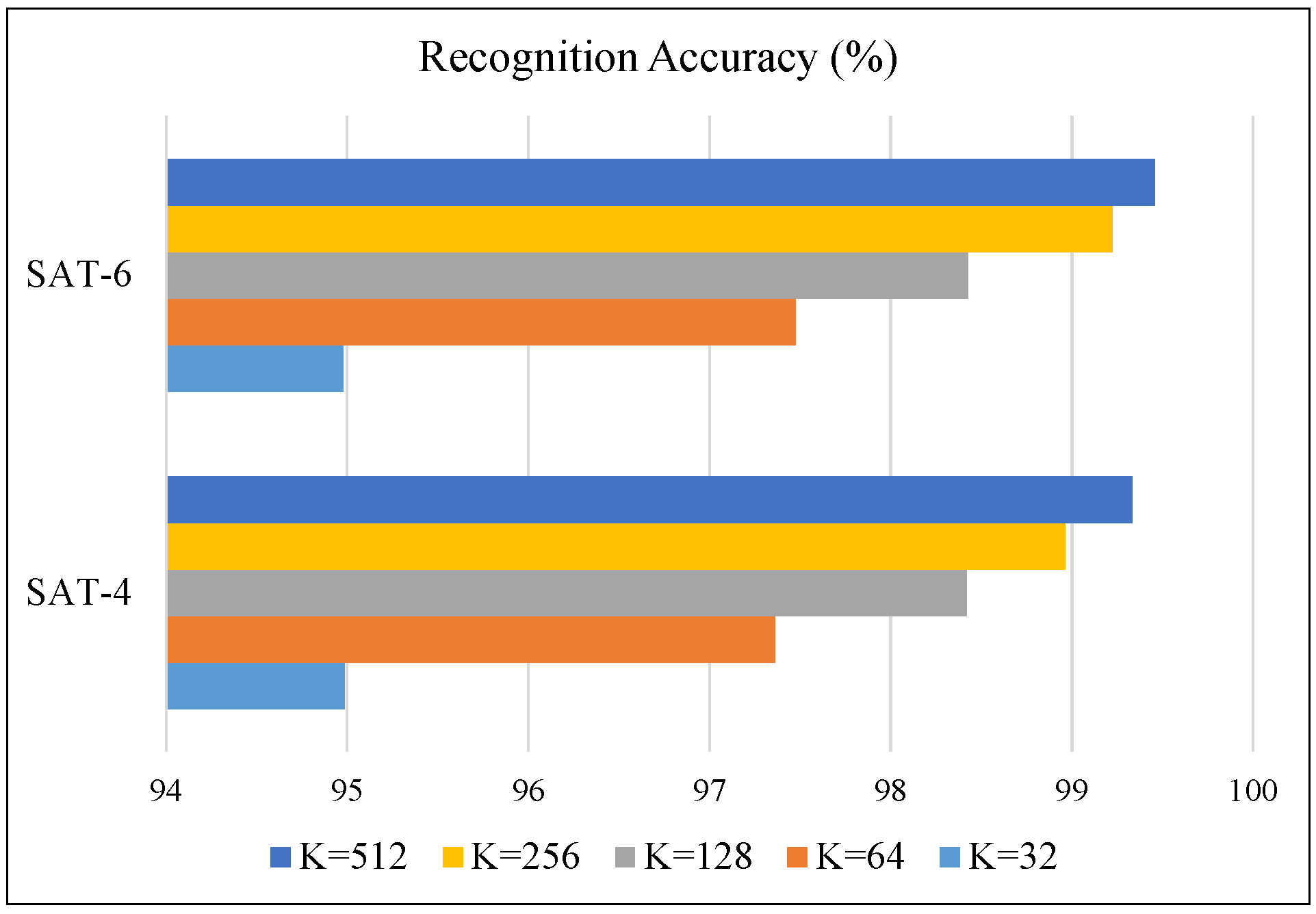
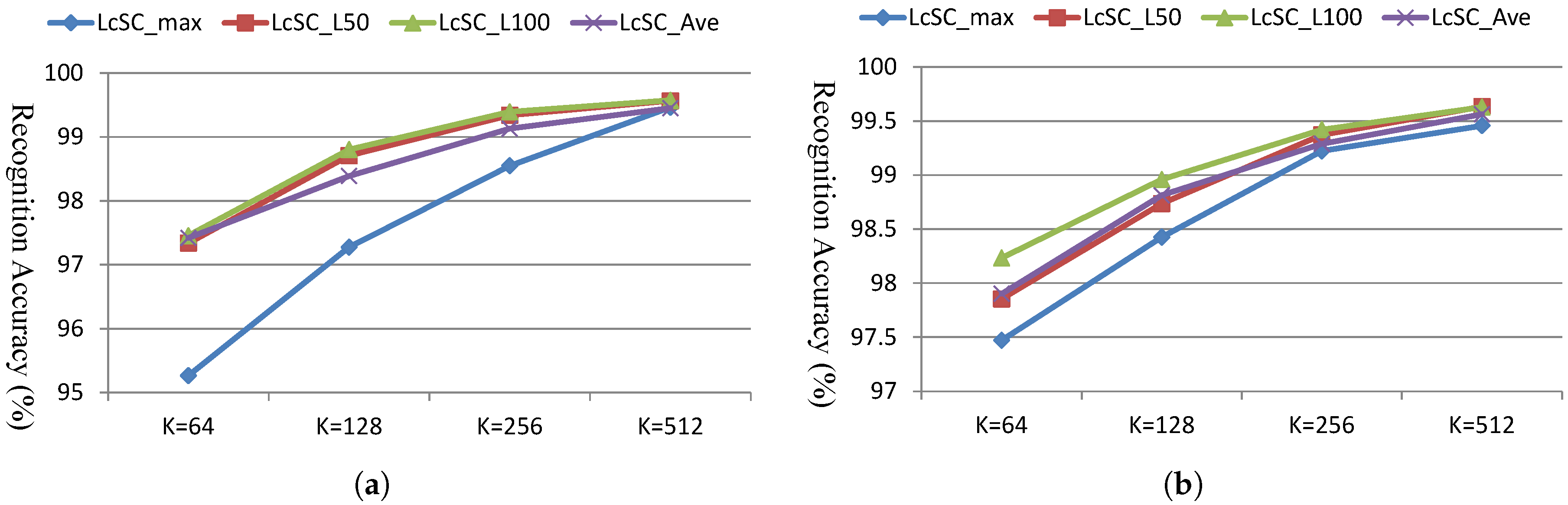
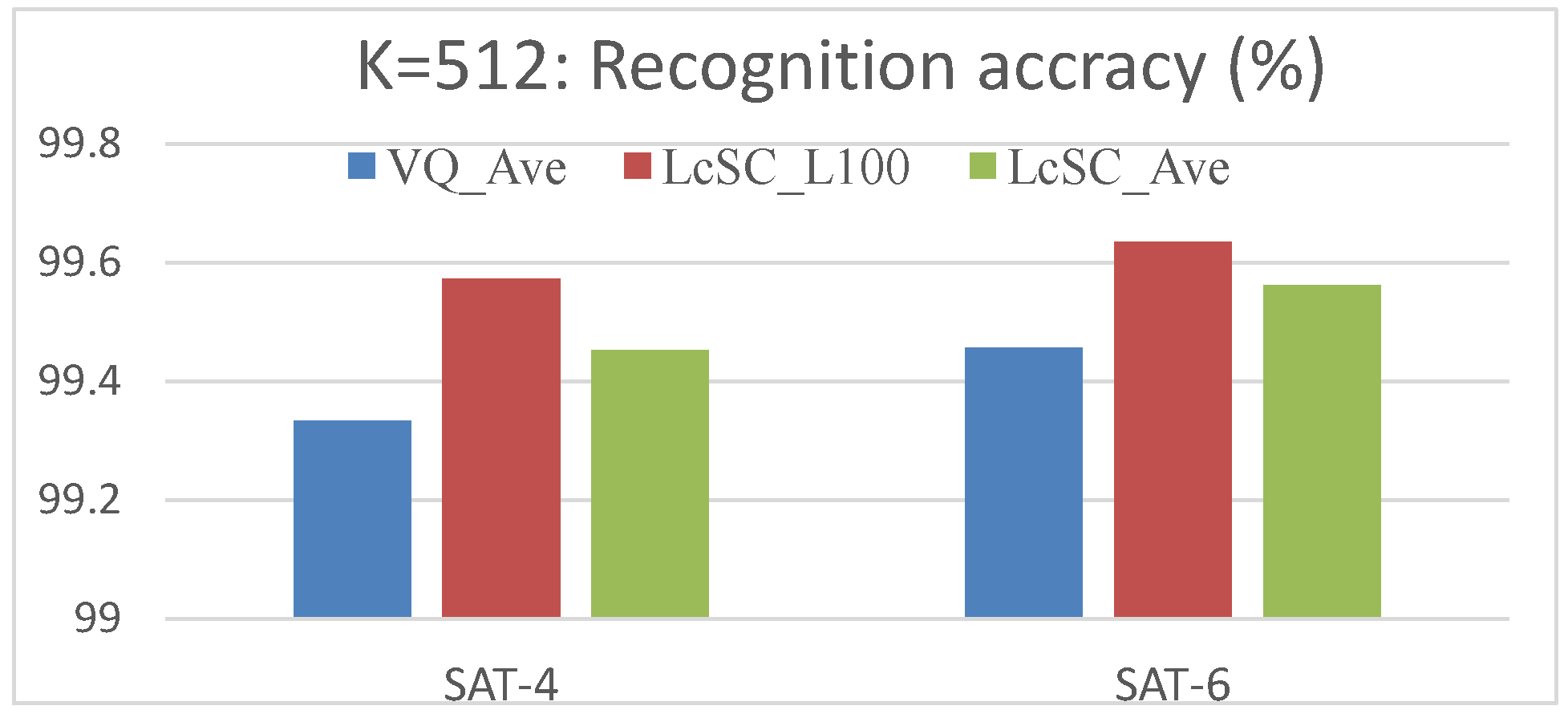
In this section, we evaluate the recognition performance on the SAT-4, SAT-6 and Megasolar datasets using our proposed multi-spectral analysis. With the aggregated coded spectral vector, we simply use a linear SVM as the classifier, which learns the classification model with the images in the training dataset and predicts the land use class label for the images of the test dataset. The recognition performances on SAT-4 and SAT-6 using the VQ coding approach combined with the average pooling strategy and different codebook sizes (K = 32, 64, 128, 256, 512) are shown in Figure 7. The results in this figure confirm the recognition performance of approximately 95% on average for both the SAT-4 and SAT-6 datasets even with the codebook size of 32 only, whereas the accuracy of more than 99% is achieved with the codebook size of 512. Next, we evaluate the recognition performances using the LcSC coding approach with different pooling methods (average: LcSC_Ave, Max: LcSC_Max; and the proposed generalized method: LcSC_L50, LcSC_L100 with the top 50 and 100 largest weights) and different codebook sizes for both SAT-4 and SAT-6 datasets, as shown in Figure 8a,b. Figure 8 shows that the proposed generalized pooling method can achieve a more accurate recognition performance than the conventional average- and max-pooling strategies under different codebook sizes. Figure 9 provides a comparison of different coding strategies (VQ and LcSC) with the codebook size of 512 on the SAT-4 and SAT-6 datasets. These results confirm the improvement of the proposed coding and pooling strategies. Table 1 contains the confusion matrix using the aggregated sparse coded vector with the LcSC coding and the proposed generalized pooling strategies under the codebook size of 512, where the recognition accuracies for all land use classes exceed 99%. Finally, the results of the performance comparison with state-of-the-art methods in [29,30] are provided. The comparison involved the application of different kinds of deep frameworks, DBN, DCN, SDE, the designed deep architectures in [29], named as DeepSat, and DCNN in [30], which integrated the inception module for taking into account the multi-scale variance in satellite images. Table 2 provides the compared average recognition accuracies on both the SAT-4 and SAT-6 datasets and reveals that our proposed framework achieves the best recognition performance.
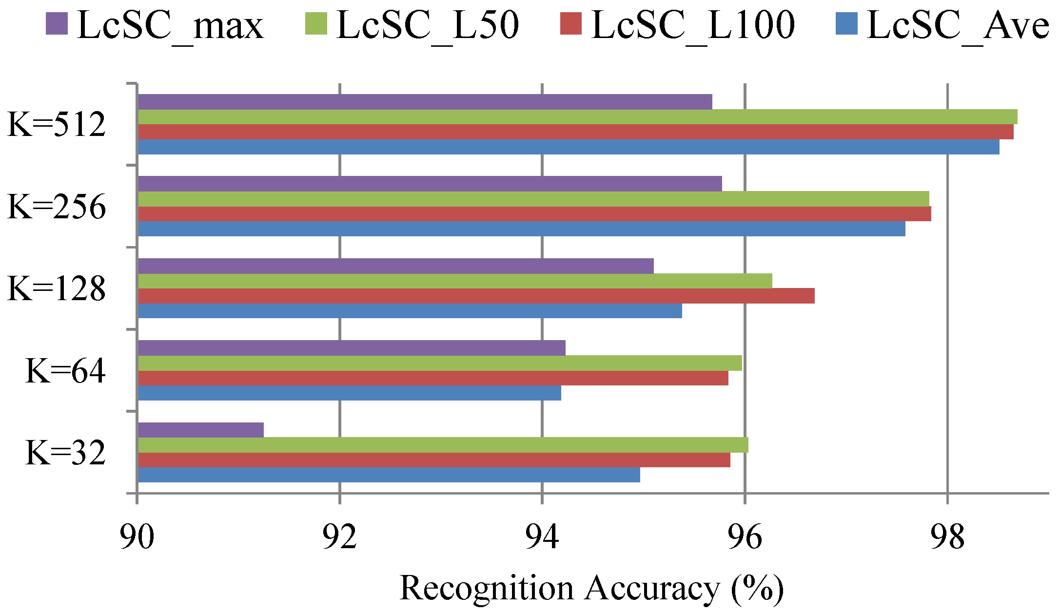
In the following, the recognition performance on the Megasolar dataset with seven spectral channels is provided. The experimental results using the LcSC coding approach with different pooling methods (average: LcSC_Ave, Max: LcSC_Max; and the proposed generalized method: LcSC_L50, LcSC_L100 with the top 50 and 100 largest weights) and different codebook sizes are given in Figure 10. Since the unbalance test sample numbers for positive and negative, the average recognition accuracy of the test positive and negative samples are computed, Figure 10 manifests that the proposed generalized pooling method can achieve a more accurate recognition performance than the conventional average- and max-pooling strategies under different codebook sizes.
4.4. Computational Cost
We implemented the proposed multi-spectral analysis and satellite image recognition system on a desktop computer with an Intel Core i5-6500 CPU. This subsection provides the processing times of the four procedures in our proposed strategy: the codebook (spectral atoms) learning (denoted as CL), SVM training (denoted as SVM-T), LcSC-based feature extraction (FE) and the label prediction with the pre-constructed SVM model (denoted SVM-P). As we know, the CL and SVM-T procedures can be implemented off-line, where CL learns the spectral atoms while SVM-T constructs a classification model with the extracted features from training images and their corresponding labels. Given any test image with an unknown class label, we need only two on-line steps: feature extraction (FE) and class label prediction with the pre-learned SVM model (SVM-P). Table 3 provides the computational times of different procedures in our proposed strategy with atom numbers: K = 256, 512, for both SAT-4 and SAT-6 datasets, where we randomly selected 500 images from each class for codebook learning. From Table 3, it can be seen that the off-line procedures take about a few hundreds of seconds for codebook learning and decades of minutes for SVM model learning, while the on-line feature extraction and SVM prediction procedures for one image are much faster with decades of millisecond only than the off-line procedure.
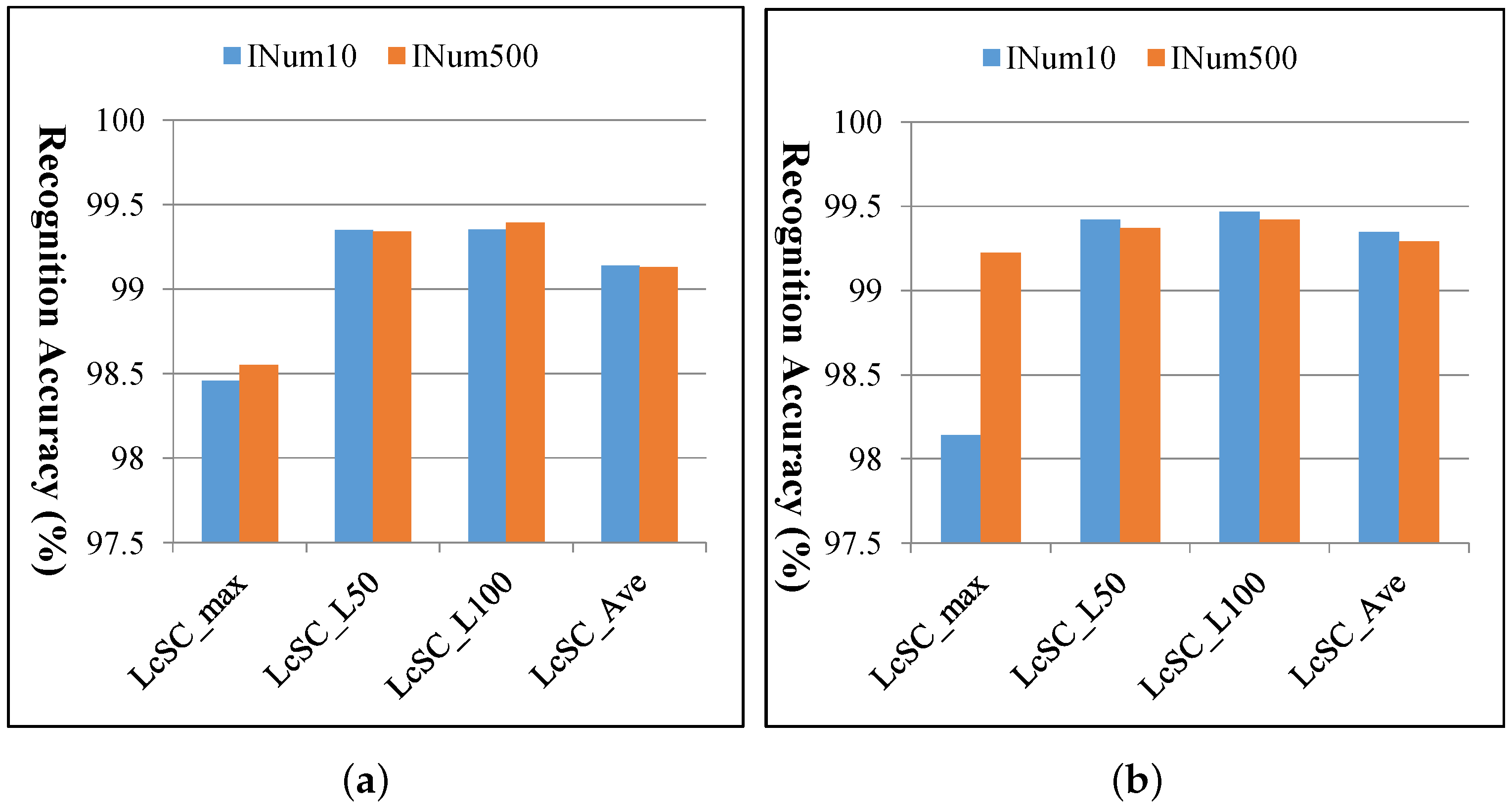
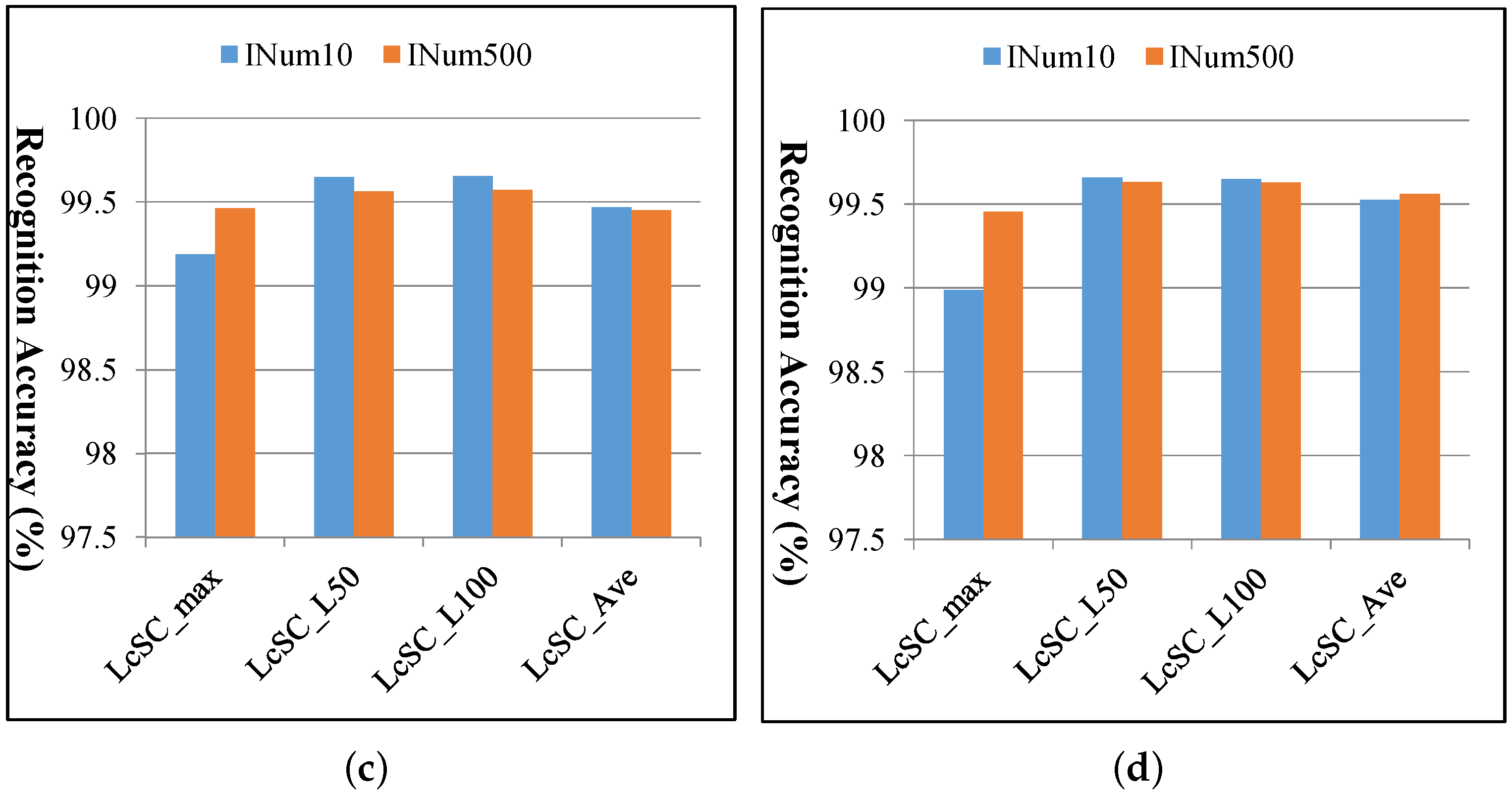
As the codebook learning for LcSC is an unsupervised procedure, it may not greatly affect the recognition performance with different numbers of images. We implemented the multi-spectral analysis strategy with the learned codebook using the randomly selected 10 images (denoted as INum10) only, instead of 500 images (denoted as INum500, in the previous experiments) from each class, and provide the compared results in Figure 11. From Figure 11, we can see that except the max-pooling-based LcSC feature, there are no obvious differences in recognition performances with the learned codebook using different image numbers, and thus, were can say that our proposed feature extraction strategy is robust to the codebook learning procedure. The processing times for codebook learning with 10 and 500 images from each class, respectively for both SAT-4 and SAT-6 datasets, are shown in Table 4, which manifests that the computational time can be greatly reduced for codebook learning with a small number of images.
5. Conclusions
This study proposed an effective and discriminative multi-spectral image representation for satellite image recognition. Due to the low resolution of the available satellite images, it would be unsuitable to conduct the spatial analysis for exploring the nearby pixel relation, and on the other hand, because of the possible available multi-spectral bands, the recognition problem may benefit from the spectral analysis. These motivated us to explore the widely-used BOW model, which achieves impressive performance for some vision applications, using the available pixel-wise multi-spectra instead of spatial analysis in the conventional method. The proposed multi-spectral analysis firstly learns the multi-spectral prototypes (dictionary) for representing any pixel-wise spectral data. Then, based on the learned dictionary, a sparse coded spectral vector for any pixel is generated with locality-constrained sparse coding techniques, which can guarantee the smoothness between the input spectral space and the coded vector space. Finally, we combined the set of coded spectral vectors in a satellite scene image to form a same-dimensional feature vector as the image representation, which we accomplished by using a generalized aggregation strategy. This strategy consisted of integrating not only the maximum magnitude, but also the response magnitude of the relatively large coded coefficients of a specific spectral prototype instead of using the conventional max- and average-pooling approaches. Experiments on three satellite datasets validated that the recognition performance of our proposed approach is comparable and impressive compared with the state-of-the-art methods for satellite scene classification.
Acknowledgments
This work was supported in part by the Grand-in Aid for Scientific Research from the Japanese Ministry for Education, Science, Culture and Sports under Grant Nos. 15K00253; We thanks Hiroki Miyamoto and Ryosuke Nakamura (AIST, Japan) for providing the database in our experiments.
Author Contributions
X.-H.H. carried out the method development, conducted experiments, and drafted the manuscript. Y.-W.C. have revised the draft critically for important intellectual content and given the final approval of the version to be published. All authors read and approved the final manuscript.
Conflicts of Interest
The authors declare no conflict of interest.
References
- Xu, Y.; Huang, B. Spatial and temporal classification of synthetic satellite imagery: Land cover mapping and accuracy validation. Geo-Spat. Inf. Sci. 2014, 17, 1–7. [Google Scholar] [CrossRef]
- Rogan, J.; Chen, D.M. Remote sensing technology for mapping and monitoring land-cover and land-use change. Prog. Plan. 2004, 61, 301–325. [Google Scholar] [CrossRef]
- Jaiswal, R.K.; Saxena, R.; Mukherjee, S. Application of remote sensing technology for land use/land cover change analysis. J. Indian Soc. Remote Sens. 1999, 27, 123–128. [Google Scholar] [CrossRef]
- Xia, G.S.; Yang, W.; Delon, J.; Gousseau, Y.; Sun, H.; Maitre, H. Structrual High-Resolution Satellite Image Indexing. In Proceedings of the ISPRS, TC VII Symposium Part A: 100 Years ISPRS, Vienna, Austria, 5–7 July 2010; pp. 298–303. [Google Scholar]
- Jiang, Y.-G.; Ngo, C.-W.; Yang, J. Towards optimal bag-of-features for object categorization and semantic video retrieval. In Proceedings of the 6th ACM International Conference on Image and Video Retrieval, Amsterdam, The Netherlands, 9–11 July 2007; pp. 494–501. [Google Scholar]
- Jurie, F.; Triggs, B. Creating efficient codebooks for visual recognition. In Proceedings of the ICCV’05, Tenth IEEE International Conference on Computer Vision, Beijing, China, 17–21 October 2005; pp. 604–610. [Google Scholar]
- Jegou, H.; Douze, M.; Schmid, C. Packing bag-of-features. In Proceedings of the ICCV’09, 12th IEEE International Conference on Computer Vision, Kyoto, Japan, 29 September–2 October 2009. [Google Scholar]
- Lazebnik, S.; Schmid, C.; Ponce, J. Beyond bags of features: Spatial pyramid matching for recognizing natural scene categories. In Proceedings of the CVPR’06, IEEE Computer Society Conference on Computer Vision, New York, NY, USA, 17–22 June 2006; pp. 2169–2178. [Google Scholar]
- Yang, J.C.; Yu, K.; Gong, Y.H.; Huang, T. Linear spatial pyramid matching using sparse coding for image classification. In Proceedings of the CVPR’09, IEEE Computer Society Conference on Computer Vision, Miami, FL, USA, 20–25 June 2009. [Google Scholar]
- Yu, K.; Zhang, T.; Gong, Y.H. Nonlinear learning using local coordinate coding. In Proceedings of the NIPS’09, Advances in Neural Information Processing Systems 22, Vancouver, BC, Canada, 7–10 December 2009; pp. 2223–2231. [Google Scholar]
- Wang, J.J.; Yang, J.C.; Yu, K.; Lv, F.J.; Huang, T.; Gong, Y.H. Locality-constrained Linear Coding for Image Classification. In Proceedings of the CVPR’10, IEEE Computer Society Conference on Computer Vision, San Francisco, CA, USA, 13–18 June 2010. [Google Scholar]
- Han, X.-H.; Chen, Y.-W.; Xu, G. High-Order Statistics of Weber Local Descriptors for Image Representation. IEEE Trans. Cybern. 2015, 45, 1180–1193. [Google Scholar] [CrossRef] [PubMed]
- Jegou, H.; Douze, M.; Schmid, C. Improving Bag-of-Features for Large Scale Image Search. Int. J. Comput. Vis. 2010, 87, 316–336. [Google Scholar] [CrossRef]
- Perronnin, F.; Sanchez, J.; Mensink, T. Improving the Fisher Kernel for Large-Scale Image Classification. In Proceedings of the ECCV2010, 11th European Conference on Computer Vision, Crete, Greece, 5–11 September 2010; pp. 143–156. [Google Scholar]
- Han, X.-H.; Wang, J.; Xu, G.; Chen, Y.-W. High-Order Statistics of Microtexton for HEp-2 Staining Pattern Classification. IEEE Trans. Biomed. Eng. 2014, 61, 2223–2234. [Google Scholar] [CrossRef] [PubMed]
- Lowe, D.G. Distinctive image features from scale-invariant keypoints. Int. J. Comput. Vis. 2004, 60, 91–110. [Google Scholar] [CrossRef]
- Yang, Y.; Newsam, S. Bag-of-visual-words and spatial extensions for land-use classification. In Proceedings of the 18th SIGSPATIAL International Conference on Advances in Geographic Information Systems, San Jose, CA, USA, 2–5 November 2010; pp. 270–279. [Google Scholar]
- Zhao, L.J.; Tang, P.; Huo, L.Z. Land-use scene classification using a concentric circle structured multiscale bag-of-visual-words model. IEEE J. Sel. Top. Appl. Earth Obs. Remote Sens. 2014, 7, 4620–4631. [Google Scholar] [CrossRef]
- Chen, S.; Tian, Y. Pyramid of Spatial Relations for Scene-Level Land Use Classification. IEEE Trans. Geosci. Remote Sens. 2014, 53, 1947–1957. [Google Scholar] [CrossRef]
- Cheriyadat, A. Unsupervised Feature Learning for Aerial Scene Classification. IEEE Trans. Geosci. Remote Sens. 2014, 52, 439–451. [Google Scholar] [CrossRef]
- Zhang, F.; Du, B.; Zhang, L. Saliency-Guided Unsupervised Feature Learning for Scene Classification. IEEE Trans. Geosci. Remote Sens. 2015, 53, 2175–2184. [Google Scholar] [CrossRef]
- Hu, F.; Xia, G.; Wang, Z.; Huang, X.; Zhang, L.; Sun, H. Unsupervised Feature Learning via Spectral Clustering of Multidimensional Patches for Remotely Sensed Scene Classification. IEEE J. Sel. Top. Appl. Earth Obs. Remote Sens. 2015, 8, 2015–2030. [Google Scholar] [CrossRef]
- Simonyan, K.; Zisserman, A. Very deep convolutional networks for large-scale image recognition. arXiv 2014. [Google Scholar]
- Jia, Y.; Shelhamer, E.; Donahue, J.; Karayev, S.; Long, J.; Girshick, R.; Guadarrama, S.; Darrell, T. Caffe: Convolutional Architecture for Fast Feature Embedding. In Proceedings of the MM2014, 22nd ACM International Conference on Multimedia, Orlando, FL, USA, 3–7 November 2014; pp. 675–678. [Google Scholar]
- Razavian, A.S.; Azizpour, H.; Sullivan, J.; Carlssonand, S. CNN features off-the-shelf: An astounding baseline for recognition. In Proceedings of the IEEE Conference on Computer Vision and Pattern Recognition Workshops, Columbus, OH, USA, 23–28 June 2014; pp. 512–519. [Google Scholar]
- Castelluccio, M.; Poggi, G.; Sansone, C.; Verdoliva, L. Land Use Classification in Remote Sensing Images by Convolutional Neural Networks. arXiv 2015. [Google Scholar]
- Penatti, O.A.B.; Nogueira, K.; Santos, J.A.D. Do Deep Features Generalize from Everyday Objects to Remote Sensing and Aerial Scenes Domains? In Proceedings of the IEEE Conference on Computer Vision and Pattern Recognition Workshops, Boston, MA, USA, 7–12 June 2015; pp. 44–51. [Google Scholar]
- Hu, F.; Xia, G.; Hu, J.W.; Zhang, L.P. Transferring Deep Convolutional Neural Networks for the Scene Classification of High-Resolution Remote Sensing Imagery. Remote Sens. 2015, 7, 14680–14707. [Google Scholar] [CrossRef]
- Basu, S.; Ganguly, S.; Mukhopadhyay, S.; Dibiano, R.; Karki, M.; Nemani, R. DeepSat—A Learning framework for Satellite Imagery. In Proceedings of the 23rd SIGSPATIAL International Conference on Advances in Geographic Information Systems, Seattle, WA, USA, 3–6 November 2015. [Google Scholar]
- Ma, Z.; Wang, Z.P.; Liu, C.X.; Liu, X.Z. Satellite imagery classification based on deep convolution network. Int. J. Comput. Autom. Control Inf. Eng. 2016, 10, 1055–1059. [Google Scholar]
- WWW2. NAIP. Available online: http://www.fsa.usda.gov/Internet/FSA$_$File/naip$_$2009$_$info$_$final.pdf (accessed on 16 March 2017).
- Zhong, Y.F.; Fei, F.; Liu, Y.F.; Zhao, B.; Jiao, H.Z.; Zhang, L.P. SatCNN: Satellite image dataset classification using agile convolutional neural networks. Remote Sens. Lett. 2017, 8, 136–145. [Google Scholar] [CrossRef]
- Adams, J.B.; Smith, M.O.; Johnson, P.E. Spectral mixture modeling: A new analysis of rock and soil types at the Viking Lander 1 site. J. Geophys. Res. 1986, 91, 8098–8112. [Google Scholar] [CrossRef]
- Settle, J.; Drake, N. Linear mixing and the estimation of ground cover proportions. Int. J. Remote Sens. 1993, 14, 1159–1177. [Google Scholar] [CrossRef]
- Plaza, A.; Martinez, P.; Perez, R.; Plaza, J. A quantitative and comparative analysis of endmember extraction algorithms from hyperspectral data. IEEE Trans. Geosci. Remote Sens. 2004, 42, 650–663. [Google Scholar] [CrossRef]
- Du, Q.; Raksuntorn, N.; Younan, N.; King, R. End-member extraction for hyperspectral image analysis. Appl. Opt. 2008, 47, 77–84. [Google Scholar] [CrossRef]
- Chang, C.-I.; Wu, C.-C.; Liu, W.; Ouyang, Y.-C. A new growing method for simplex-based endmember extraction algorithm. IEEE Trans. Geosci. Remote Sens. 2006, 44, 2804–2819. [Google Scholar] [CrossRef]
- Zare, A.; Gader, P. Hyperspectral band selection and endmember detection using sparsity promoting priors. IEEE Trans. Geosci. Remote Sens. 2008, 5, 256–260. [Google Scholar] [CrossRef]
- Zortea, M.; Plaza, A. A quantitative and comparative analysis of different implementations of N-FINDR: A fast endmember extraction algorithm. IEEE Trans. Geosci. Remote Sens. 2009, 6, 787–791. [Google Scholar] [CrossRef]
- Bay, H.; Ess, A.; Tuytelaars, T.; Gool, L.V. SURF: Speeded Up Robust Features. Comput. Vis. Image Underst. 2008, 110, 346–359. [Google Scholar] [CrossRef]
- Ishii, T.; Edgar, S.-S.; Iizuka, S.; Mochizuki, Y.; Sugimoto, A.; Ishikawa, H.; Nakamura, R. Detection by classification of buildings in multispectral satellite imagery. In Proceedings of the International Conference on Pattern Recognition (ICPR), Cancun, Mexico, 4–8 December 2016. [Google Scholar]
Figure 1.
Proposed satellite image representation framework. The top row manifests the learning procedure of the multi-spectral prototypes, whereas the bottom row denotes the coding and pooling procedure of the pixel-wise multi-spectra in images to provide the final representation vector.
Figure 1.
Proposed satellite image representation framework. The top row manifests the learning procedure of the multi-spectral prototypes, whereas the bottom row denotes the coding and pooling procedure of the pixel-wise multi-spectra in images to provide the final representation vector.

Figure 2.
Bag-of-visual-words model for image representation.

Figure 3.
Flowchart of the linear unmixing model.

Figure 4.
Some sample images. (a) Sample images from the SAT-4 dataset. Each row denotes a class of images, and from top to bottom, the classes are barren land, trees, grassland and others, respectively. (b) Sample images from the SAT-6 dataset. Each row denotes a class of images, and from top to bottom, the classes are buildings, barren land, trees, grassland, roads and water bodies, respectively.

Figure 5.
Plotted spectra of four learned multi-spectral prototypes (MSP) from the SAT-4 dataset, named MSP1, MSP2, MSP3, MSP4, respectively.
Figure 5.
Plotted spectra of four learned multi-spectral prototypes (MSP) from the SAT-4 dataset, named MSP1, MSP2, MSP3, MSP4, respectively.

Figure 6.
Image number statistics of the aggregated coefficients for different learned multi-spectral prototypes and the SAT-4 training dataset. (a) The image frequency of different land use classes between different aggregated coefficient regions of the MSP1 in Figure 5; (b) for the MSP2 in Figure 5; (c) for the MSP3 in Figure 5; (d) for the MSP4 in Figure 5.


Figure 7.
Recognition accuracies of the proposed multi-spectral representation based on the vector quantization (VQ) coding strategy under different codebook sizes (K = 32, 64, 128, 256, 512) for both datasets SAT-4 and SAT-6.
Figure 7.
Recognition accuracies of the proposed multi-spectral representation based on the vector quantization (VQ) coding strategy under different codebook sizes (K = 32, 64, 128, 256, 512) for both datasets SAT-4 and SAT-6.

Figure 8.
Recognition accuracies of the proposed multi-spectral representation based on LcSC coding and different pooling strategies (LcSC_Max: Max pooling; LcSC_Ave: average pooling; LcSC_L50: the proposed generalized pooling method with the top 50 coefficients; LcSC_L100: the proposed generalized pooling method with the top 100 coefficients) under codebook sizes (K = 64, 128, 256, 512) for both datasets: (a) SAT-4 and (b) SAT-6.

Figure 9.
Compared recognition accuracies based on VQ and LcSC coding strategies for codebook size: K = 512 for both datasets SAT-4 and SAT-6.
Figure 9.
Compared recognition accuracies based on VQ and LcSC coding strategies for codebook size: K = 512 for both datasets SAT-4 and SAT-6.

Figure 10.
Recognition accuracies of the proposed multi-spectral representation based on LcSC coding and different pooling strategies under codebook sizes (K = 32, 64, 128, 256, 512) for the Megasolar dataset.
Figure 10.
Recognition accuracies of the proposed multi-spectral representation based on LcSC coding and different pooling strategies under codebook sizes (K = 32, 64, 128, 256, 512) for the Megasolar dataset.

Figure 11.
Comparison of the recognition accuracies of the proposed multi-spectral representation based on LcSC coding with the learned codebook using 10 and 500 images, respectively, from each class for both the SAT-4 and SAT-6 datasets. The compared accuracies with (a) codebook size: K = 256 for SAT-4, (b) codebook size: K = 512 for SAT-4, (c) codebook size: K = 256 for SAT-6 and (d) codebook size: K = 512 for SAT-6.


Table 1.
Confusion matrix using locality-constraint sparse coding (LcSC) coding and the proposed generalized pooling strategy with codebook size K = 512 for both SAT-4 and SAT-6 datasets.
Table 1.
Confusion matrix using locality-constraint sparse coding (LcSC) coding and the proposed generalized pooling strategy with codebook size K = 512 for both SAT-4 and SAT-6 datasets.
| (a) SAT-4 | ||||||
| (%) | Barren Land | Trees | Grassland | Others | ||
| Barren land | 99.404 | 0 | 0.554 | 0.042 | ||
| Trees (linear) | 0 | 99.97 | 0.035 | 0 | ||
| Grassland | 0.407 | 0.061 | 99.515 | 0.017 | ||
| Others | 0.034 | 0.003 | 0.003 | 99.961 | ||
| (b) SAT-6 | ||||||
| (%) | Building | Barren Land | Trees | Grassland | Road | Water |
| Building | 100 | 0 | 0 | 0 | 0 | 0 |
| Barren land | 0 | 99.134 | 0 | 0.866 | 0 | 0 |
| Trees | 0 | 0 | 99.894 | 0.106 | 0 | 0 |
| Grassland | 0.008 | 0.802 | 0.143 | 99.047 | 0 | 0 |
| Road | 0 | 0 | 0 | 0 | 100 | 0 |
| Water | 0 | 0 | 0 | 0 | 0 | 100 |
| Methods | SAT-4 | SAT-6 |
|---|---|---|
| DBN [29] | 81.78 | 76.41 |
| CNN [29] | 86.83 | 79.06 |
| SDAE [29] | 79.98 | 78.43 |
| Semi-supervised [29] | 97.95 | 93.92 |
| DCNN [30] | 98.408 | 96.037 |
| Ours | 99.709 | 99.679 |
Table 3.
Computational times of different procedures in our proposed strategy. CL, FE, SVM-T and SVM-P denote codebook learning, feature extraction, SVM training and SVM prediction, respectively, while ’s’ and ’m’ represent second and minute and CB size denotes codebook size, respectively.
Table 3.
Computational times of different procedures in our proposed strategy. CL, FE, SVM-T and SVM-P denote codebook learning, feature extraction, SVM training and SVM prediction, respectively, while ’s’ and ’m’ represent second and minute and CB size denotes codebook size, respectively.
| CB Size | Off-Line | On-Line | ||||
|---|---|---|---|---|---|---|
| CL(s) | SVM-T(m) | FE(s) | SVM-P(s) | |||
| SAT-4 | SAT-6 | SAT-4 | SAT-6 | For one 28 × 28 image | ||
| Dict:256 | 270.40 | 393.17 | 42.62 | 9.54 | 0.024 | 0.010 |
| Dict:512 | 530.96 | 906.17 | 52.89 | 11.25 | 0.038 | 0.014 |
Table 4.
Processing time (s) for codebook learning with 10 and 500 images, respectively, for both SAT-4 and SAT-6 datasets.
Table 4.
Processing time (s) for codebook learning with 10 and 500 images, respectively, for both SAT-4 and SAT-6 datasets.
| Codebook Size | SAT-4 | SAT-6 | ||
|---|---|---|---|---|
| INum10 | INum500 | INum10 | INum500 | |
| K = 256 | 4.54 | 270.40 | 6.61 | 393.17 |
| K = 512 | 7.37 | 530.96 | 12.57 | 906.17 |
© 2017 by the authors. Licensee MDPI, Basel, Switzerland. This article is an open access article distributed under the terms and conditions of the Creative Commons Attribution (CC BY) license (http://creativecommons.org/licenses/by/4.0/).
Share and Cite
MDPI and ACS Style
Han, X.-H.; Chen, Y.-w. Generalized Aggregation of Sparse Coded Multi-Spectra for Satellite Scene Classification. ISPRS Int. J. Geo-Inf. 2017, 6, 175. https://0-doi-org.brum.beds.ac.uk/10.3390/ijgi6060175
AMA Style
Han X-H, Chen Y-w. Generalized Aggregation of Sparse Coded Multi-Spectra for Satellite Scene Classification. ISPRS International Journal of Geo-Information. 2017; 6(6):175. https://0-doi-org.brum.beds.ac.uk/10.3390/ijgi6060175
Chicago/Turabian StyleHan, Xian-Hua, and Yen-wei Chen. 2017. "Generalized Aggregation of Sparse Coded Multi-Spectra for Satellite Scene Classification" ISPRS International Journal of Geo-Information 6, no. 6: 175. https://0-doi-org.brum.beds.ac.uk/10.3390/ijgi6060175
Note that from the first issue of 2016, this journal uses article numbers instead of page numbers. See further details here.