Trajectory Data Mining via Cluster Analyses for Tropical Cyclones That Affect the South China Sea

Abstract

The equal division of tropical cyclone (TC) trajectory method, the mass moment of the TC trajectory method, and the mixed regression model method are clustering algorithms that use space and shape information from complete TC trajectories. In this article, these three clustering algorithms were applied in a TC trajectory clustering analysis to identify the TCs that affected the South China Sea (SCS) from 1949 to 2014. According to their spatial position and shape similarity, these TC trajectories were classified into five trajectory classes, including three westward straight-line movement trajectory clusters and two northward re-curving trajectory clusters. These clusters show different characteristics in their genesis position, heading, landfall location, TC intensity, lifetime and seasonality distribution. The clustering results indicate that these algorithms have different characteristics. The equal division of the trajectory method provides better clustering result generally. The approach is simple and direct, and trajectories in the same class were consistent in shape and heading. The regression mixture model algorithm has a solid theoretical mathematical foundation, and it can maintain good spatial consistency among trajectories in the class. The mass moment of the trajectory method shows overall consistency with the equal division of the trajectory method.

1. Introduction

Tropical cyclones (TCs) are a type of intense atmospheric cyclonic eddy generated over warm tropical oceans [1]. They are one of the most globally devastating natural catastrophes and usually have a considerable socio-economic impact for countries in TC-prone areas [2,3,4]. The South China Sea (SCS), which is the largest semi-enclosed marginal sea in the Northwest Pacific, is also an active region of TCs. Approximately 13.2% of the TCs formed in the Western North Pacific (WNP) were generated in the SCS [5]. In addition, more than 60% of the TCs in the WNP affect countries and areas located around the SCS [6]. Previous studies have primarily focused on WNP TCs in general [7,8,9,10,11,12,13,14], whereas relatively few studies have focused on the specific characteristics of TCs affecting the SCS. With the rapid social economic development and population growth in the areas around the SCS, it is important to gain a better understanding of how TC behaviour affects the SCS.

TC landfall locations are primarily determined by their trajectories [15]; therefore, identifying the rules of TCs trajectories represents one of the most important aspects of TC disaster protection [16]. Previous studies have found that the characteristics of these TC trajectories can be better understood by classifying them into several clusters [9,11,14]. For example, by classifying TC trajectories into three types (straight-moving storms, re-curving-south storms, and re-curving-north storms), Harry and Elsberry [11] illustrated the relationship between TC trajectory types and anomalous 700-mb large-scale circulation patterns and TC genesis locations. Hodnish and Gray [9] investigated features of environmental wind fields at all levels of the troposphere that are related to TC re-curvature by categorizing TCs into four patterns: non-re-curving cyclones, sharply re-curving cyclones, gradually re-curving cyclones and left-turning cyclones. Lander [14] discussed the effects of the reverse orientation of the summer monsoon trough of the WNP further north and east than normal for TC motion by classifying TC trajectories into four major patterns: straight moving, re-curving, north oriented and SCS oriented.

However, the results of previous studies were relatively qualitative and descriptive; therefore, more effective quantitative methods are needed to better understand the behaviour of TC trajectories. The numerical clustering method includes objective characteristics and represents a quantitative data-mining method that is widely applied in many areas, including public transportation [17,18], the humanities and social sciences (e.g., Twitter events) [19,20,21], and environmental pollution [22,23,24]. Compared with other clustering objects, TCs with different lifetimes generate tracks with different lengths; thus, they cannot be analysed through the direct use of common clustering methods. To overcome this shortcoming, different methods have been proposed. Some studies included special trajectory points and the K-means clustering method [25] to perform cluster analyses of TC trajectories. Based on the geographical position of TCs at their maximum intensity and terminal position, Elsner and Liu studied the WNP and the North Atlantic TCs by classifying them into three clusters [10,26]. Blender used six-hourly trajectory point positions over three days to cluster trajectories of extratropical TCs in the North Atlantic [27], and Corporal-Lodangco and Leslie clustered TCs affecting the Philippines based on their genesis, maximum intensity, and decay point positions [28].

However, these methods are exclusively based on limited special points of the TC track, and Gaffney [29] suggested that this method is not desirable for resolving the problem because the features of TC trajectories should be expressed by the entire TC trajectory [29,30]. To overcome the deficiencies of these methods, Gaffney proposed a Finite-Mixture-Model (FMM) clustering algorithm [29,31], which has been utilized in many TC trajectory clustering analyses of the WNP [30,32], the North Atlantic Ocean [33,34], the Eastern North Pacific Ocean [35], and the North Indian Ocean [36]. Nakamura et al. proposed the use of two mass moments of TC trajectory, namely, the centroid and the variance (x-, y-, and xy-directions), for TC trajectory clustering. These two mass moments reflect the TC position and shape separately and constitute a vector of five scalar components per TC track. By applying the mass moments to the K-means clustering method, a reliable clustering result of six clusters for the North Atlantic TCs were obtained [34]. Kim also solved this problem and analysed the WNP TCs by dividing each trajectory into M segments of equal length [6]. Through sufficient density of equal dividing sample points, the original position and shape character of each trajectory can be retained. Therefore, the common clustering method can be used to cluster the re-sampled TC tracks.

TCs that affect the SCS include not only the TCs forming locally in the SCS but also the TCs forming in the WNP and then migrating into the SCS. Therefore, it would be more appropriate to incorporate all these TCs in the TC trajectory analysis to obtain a more comprehensive understanding of the trajectory characteristics of TCs that affect the SCS. However, few studies have focused on the unique TC trajectory characteristics of the SCS, especially using quantitative numeric clustering methods [37,38]. In this paper, we use the three abovementioned methods based on full TC trajectory information to perform TC trajectory clustering and analyse the TC trajectory patterns that affect the SCS. Comparisons of the results of these methods are performed, and their differences are analysed.

2. Research Methods

2.1. Research Data

In this paper, the best-track dataset for TCs from 1949 to 2014 provided by the China Meteorological Administration (CMA) was adopted. This dataset provides the longitude and latitude for the spatial location, the maximum sustained wind velocity, and lowest pressure near the centre of TCs every six hours in the WNP (to the north of the equator and the west of longitude 180° E, including the SCS) since 1949. Because there are more observations of TCs in the continental and surrounding sea areas of China, this dataset has more advantages in the areas surrounding China and the SCS [39,40].

The spatial range in this study is within the region (105°–125° E, 0°–27° N), which covers the entire SCS and the surrounding areas and countries. When a TC generated in the WNP passes through this region, it is selected as a TC that has an impact on the SCS. Only TCs with a maximum wind velocity ($v_{max}$) above the tropical storm threshold (17.2 m/s $\le v_{max}$) were adopted. Overall, 946 TC trajectories were selected. We also conducted a clustering analysis for the TC trajectories after 1972, the year in which satellite observation techniques began to be used. According to the results, there are no essential differences in the analysis results compared with data recorded since 1949, lending credibility to the trajectory data of the TCs recorded in the dataset.

2.2. Equal Division of TC Trajectory Method

Equally dividing a trajectory into M parts is a simple and straightforward method of processing trajectory data of different lengths. In the actual application, the equivalent trajectory division points can be extracted using available tools, such as the ICurve.QueryPoint method of the ArcGIS Engine.

For random variables that obey the Gaussian distribution, more than 99% of the values of the random variable are contained in the range of (μ − 3σ, μ + 3σ), where μ is the average, and σ is the standard deviation of the random variable. According to the central limit theorems, the lifetime of a TC can be assumed to obey the Gaussian distribution. The statistical result shows that the average lifetime of TCs in the dataset is μ = 178 h, and the standard deviation is σ = 80 h. Because the TC trajectory obtains each sampling point for every six-hour time interval, we selected 80 equal division sample points for each TC track. Therefore, the coordinate points of each TC trajectory are organized into a 1 × 160 row vector, $Tr{j}_i={\left[{\tilde{x}}_1, {\tilde{y}}_1, \cdots , {\tilde{x}}_{80}, {\tilde{y}}_{80}\right]}_{1\times 160}$. The ensemble of all TC tracks in the dataset will constitute a k × 160 matrix, ${\tilde{X}}_k={\left[Tr{j}_1, \cdots , Tr{j}_k\right]}^T$, and k = 946 is the number of TC trajectories.

2.3. Mass Moment of the TC Trajectory Method

Using the mass moment of the trajectory, the shape and length of the entire trajectory can be comprehensively considered in the clustering process. This method includes two mass moments, the first of which is represented by the coordinates $\left(\overline{x},\overline{y}\right)$ for the central point position of the trajectory. The equation is as follows:

$$\mathrm{M}1=\frac{1}{A}{\displaystyle \int }w\left(r\right)rdxdy=\frac{1}{{{\displaystyle \sum }}_{i=1}^{n}w\left(r_i\right)}{{\displaystyle \sum }}_{i=1}^{n}w\left(r_i\right)r_i,$$

(1)

where r is the coordinate vector (x, y) for a point on the trajectory, w(r) is the value corresponding to the selected weight variable (such as the intensity of TC) at that point, and A is a constant represented by the integral of the selected weight variable on the overall trajectory. The form of the polynomial sum on the right side of the equation is an approximate simplified calculation of this value using n discrete observation points in the trajectory. M1 is the geometric centre of the trajectory, representing its location.

The second matrix represents the variance of coordinates x, y of the trajectory, and the corresponding mathematical form is as follows:

$$\mathrm{M}2=\frac{1}{A}{\displaystyle \int }w\left(r\right){\left(r-M1\right)}^{2}dxdy=\frac{1}{{{\displaystyle \sum }}_{i=1}^{n}w\left(r_i\right)}{{\displaystyle \sum }}_{i=1}^{n}w\left(r_i\right){\left(r_i-M{1}_i\right)}^2.$$

(2)

The variable symbols in this equation are equivalent to the corresponding symbols in the equation for M1 [34]. In this paper, we cluster the TC trajectories according to the shape characteristics of the trajectory, and the value of w at different points is set to one. The expression form of matrix M2 is $\mathrm{M}2=\left[\begin{array}{cc}{\sigma }_x^2& {\sigma }_{xy}\\ {\sigma }_{yx}& {\sigma }_y^2\end{array}\right].$ This matrix corresponds to a variance ellipse that represents the shape of the trajectory. The long axis of the ellipse reflects the direction and range for the maximum distribution of the trajectory points, and the short axis of the ellipse reflects the degree of concentration for the distribution of the trajectory points in this direction. The angle of the long axis is determined by the covariance, which reflects the overall moving trend of the trajectory.

Through this transformation, each trajectory is expressed by a five-dimensional vector, i.e., $\left[\overline{x},\overline{y},{\sigma }_x^2,{\sigma }_y^2,{\sigma }_{xy}\right]$. For the coordinate elements and variance elements in the vector to have the same order of magnitude, the variables must be normalized. In addition, we assign the weight for each coordinate variable as ${\rho }_1=0.5/2$ and the weight for each variance variable as ${\rho }_2=0.5/3$. Thus, the position and shape factors of the trajectory have the same effect on the clustering results.

Kim [6] suggested that compared with hard clustering methods such as K-means, fuzzy clustering methods allow each object to belong to all clusters with assigned corresponding membership coefficients (ranging from 0 to 1) that evaluate the degree to which an object belongs to each of clusters. Thus, fuzzy clustering can better manage fuzzy datasets such as TC trajectories, which are too complex to determine the potential boundaries and discrete different patterns. Chu [41] also argues that the fuzzy c-means (FCM) algorithm is more suitable for TC track data. Therefore, in this paper, the FCM clustering algorithm is selected to perform cluster analyses of TC trajectories in both the mass moment method and the equal division method.

2.4. Mixed Regression Model Method

The mixed regression model uses the linear combination of a finite number of density functions to express the distribution of data, and the Expectation Maximum (EM) algorithm is used to perform the clustering analysis of the trajectory data. In the regression mixture model, coordinates x and y of each observation point in the trajectory are expressed in the form of a p-order polynomial function with respect to observation time t, $\mathrm{z}={\beta }_p{t}^p+{\beta }_{p-1}{t}^{p-1}+\cdots +{\beta }_1{t}^1+{\beta }_0$. The form of the function for the regression polynomial fitting of each trajectory is as follows:

$$z_i=T_i\beta +{\epsilon }_i,$$

(3)

where $z_i={\left[X, Y\right]}_{n_i\times 2}$, X, Y are the column vector of the x coordinate and the y coordinate for the trajectory, respectively; $T_i$ is the n_i × (p + 1) Vandermonde determinant; and β is the (p + 1) × 2 matrix of the regression coefficients. The first column in the matrix is the regression coefficient of the x coordinate on the TC trajectory, the second column is the regression coefficient of the y coordinate. ε_i is the n_i × 2 error term that obeys the normal distribution; its average is 0, and n_i is the number of points in the trajectory. According to the number of observation points in the trajectory, n_i can take different values. Based on the qualitative artificial method and the quantitative analysis used to determine the fitting results for the TC trajectory, Gaffney suggested that the quadratic polynomial has the best fitting result for the TC trajectory [42]. Therefore, quadratic polynomials are typically used for clustering analyses of TC trajectories. In this paper, we also adopt the quadratic polynomial method to perform the clustering analysis of TCs in the SCS.

The conditional density function for the ith trajectory is as follows:

$$p\left(z_i|t_i,\theta \right)=f(z_i|T_i\beta ,{\displaystyle \sum })={\left(2\pi \right)}^{-n_i/2}exp\left[-\frac{1}{2}tr\left(z_i-T_i\beta \right){{\displaystyle \sum }}^{-1}{\left(z_i-T_i\beta \right)}^{\prime }\right].$$

(4)

According to the definition of the mixture model, when there are k functions of probability density, the probability density function of the trajectory i is as follows:

$$p\left(z_i|t_i,\psi \right)={{\displaystyle \sum }}_k^K{\alpha }_k{p}_k(z_i|t_i,{\theta }_k)={{\displaystyle \sum }}_k^K{\alpha }_k{f}_k(z_i|T_i{\beta }_k,{{\displaystyle \sum }}_k).$$

(5)

For the dataset that contains n typhoon trajectories, $Z=\left\{z_1,\cdots ,z_n\right\}$, the overall probability density is the product of the different trajectory probability densities in set Z, such as Equation (6), where $T_i=\left\{t_1,\cdots ,t_n\right\}$ is the observation time of different typhoon trajectories:

$$p(Z|T,\psi )={{\displaystyle \prod }}_i^n{{\displaystyle \sum }}_k^K{\alpha }_k{f}_k(z_i|T_i{\beta }_k,{{\displaystyle \sum }}_k).$$

(6)

Using the observed coordinate data of TC trajectories and the EM algorithm, the probability for each trajectory as the member of the kth density function is obtained. By dividing the trajectory into the function with the largest probability, the clustering of TC tracks is achieved.

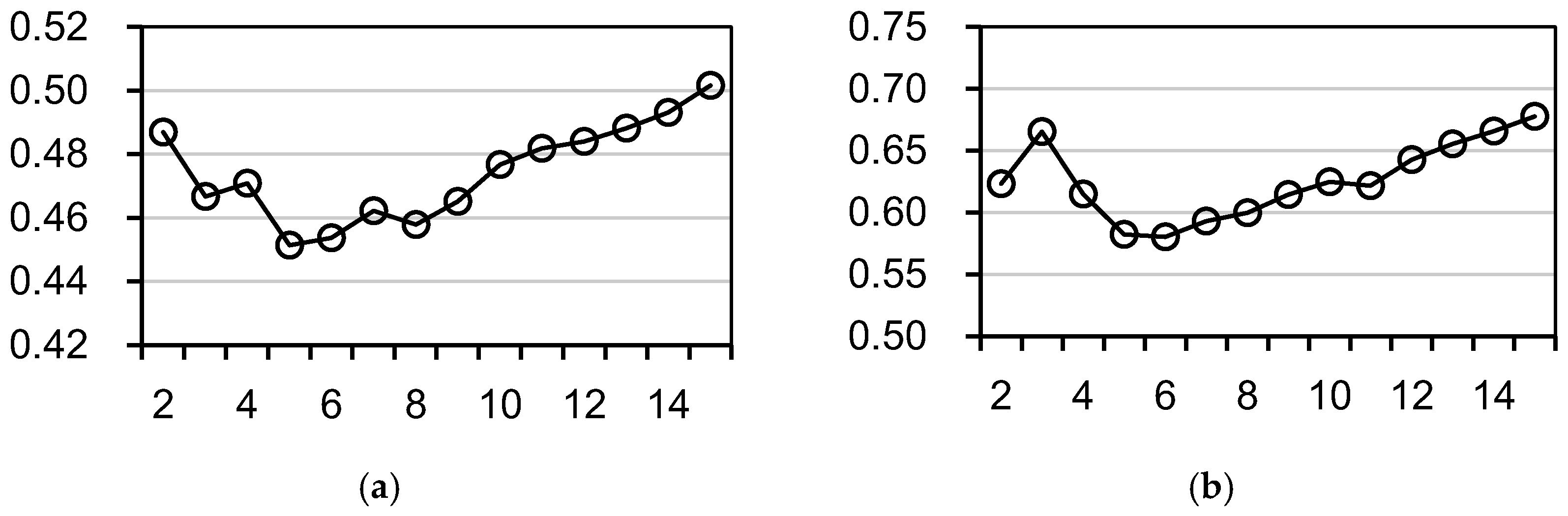
2.5. Selection of the Number of Clusters

Determining the optimum number of clusters is an important process performed in clustering analysis. To determine the optimum number of clusters, Figure 1 shows the coefficients of variation index values obtained by the equal division of the trajectory and the mass moment of the trajectory methods. The coefficient of variation represents the ratio between the standard deviation and the average of the total distances of all the TC trajectories to their cluster centres, and this value reflects the overall degree of dispersion for TC trajectories to their class centres. Smaller values for the index correspond to better clustering results. The index shows that when the number of clusters is set to five or six, relatively good clustering results can be obtained. We also used indices such as average similarity [43], the partition index [44], and the log-likelihood index [30], and a comprehensive comparison of different indices was performed to determine the optimum number of clusters [45]. All these indices showed consistent results with the coefficient of variation index. Compared with previous studies on the clustering analysis of TCs in the entire WNP, both Camargo [30] and Kim [6] selected seven as the optimum number of clusters. However, this paper includes only the TCs that affect the region of the SCS. Therefore, by summarizing the above analyses, we select five classes as the optimum number of clusters.

3. Results

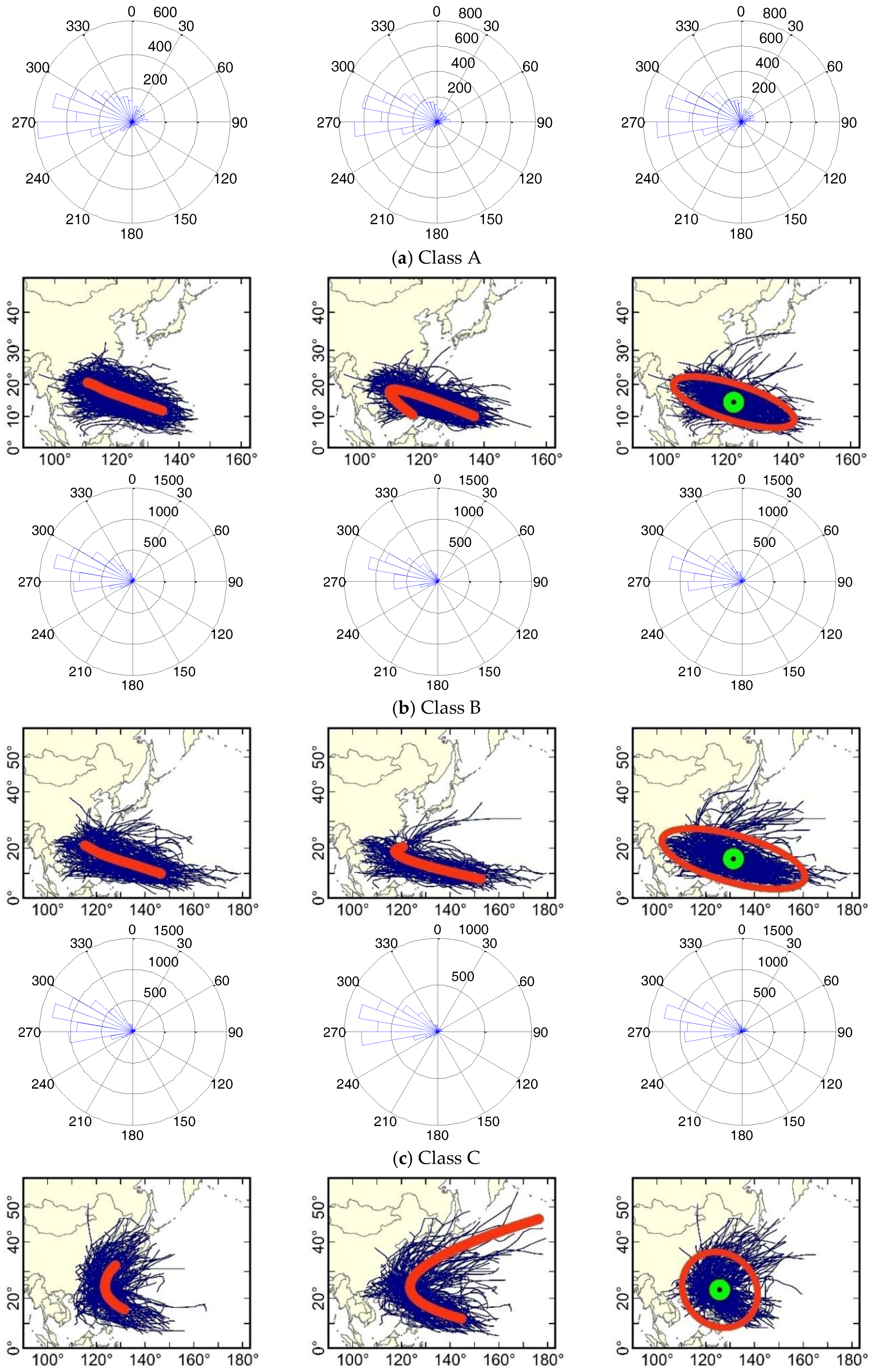
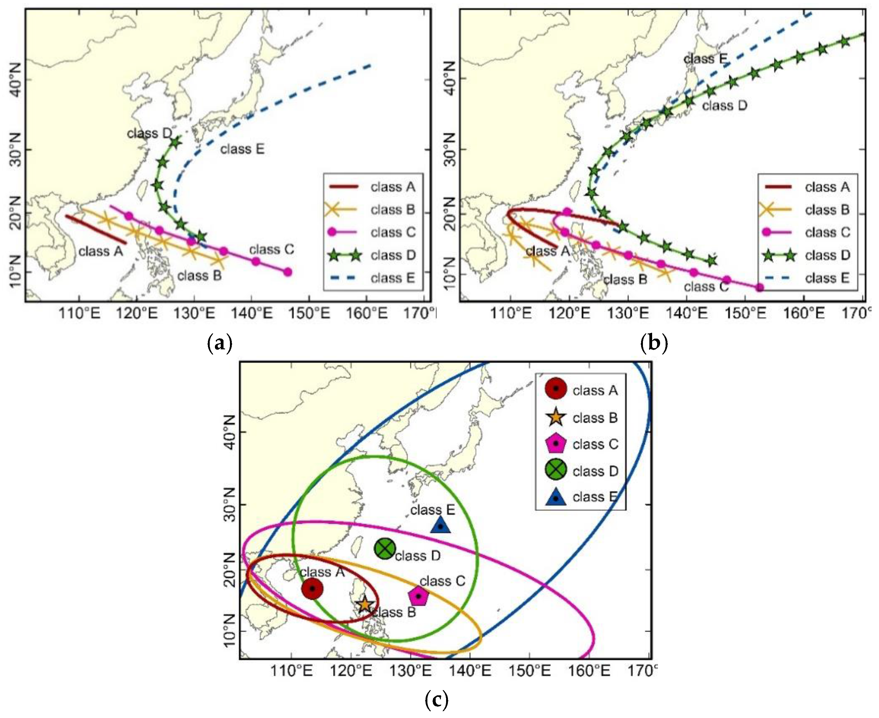
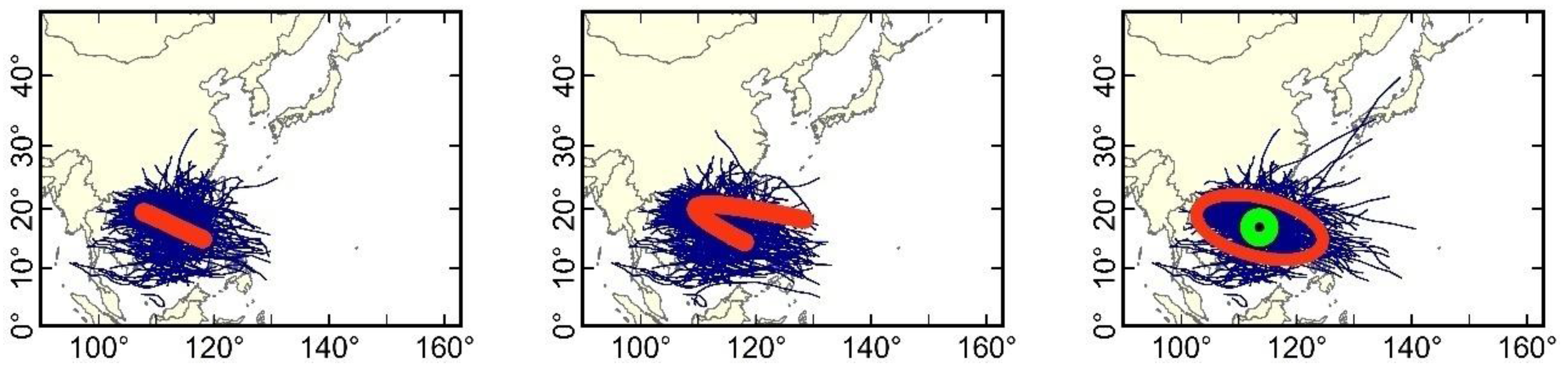
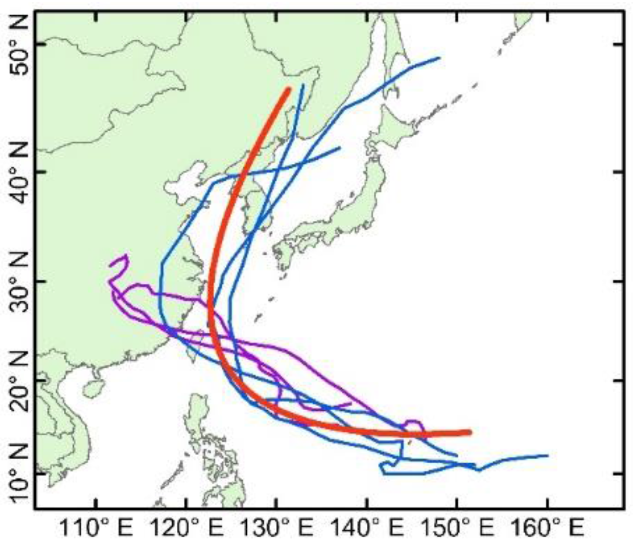
3.1. Clustering Results for the TC Trajectories

The clustering centre represents the overall characteristics and tendency of elements in the class. Figure 2 shows the clustering centres obtained by various clustering methods. This figure shows that the clustering centres of the equal division of the trajectory method (Figure 2a) and the mixed regression model method (Figure 2b) are both curved, representing the average spatial location and moving features of their class. The results for the mass moment of the trajectory method (Figure 2c) show the average of variance ellipses for the different element trajectories in the class, and the average ellipses provide an expression of the spatial distribution of the trajectory. To facilitate the comparison among the results of the three methods, classes with similar location and shape properties are sorted into the same group, and a class number is assigned and sequentially marked as class A, class B, class C, class D, and class E.

In general, the different algorithms all obtain three classes of westward straight-moving trajectories and two classes of northward re-curving trajectories for the TCs affecting the SCS. The class centres of the three straight-moving classes are sequentially shifted east from the SCS basin to approximately 150° E. Therefore, the corresponding average length of the trajectory also gradually increases (

Table 1. Statistics for the length of the tropical cyclone (TC) trajectories in each category.

TC Trajectory Class	Equal Division of the Trajectory Method		Mixed Regression Model Method		Mass Moment of the Trajectory Method
	Average Length (km)	Standard Deviation (km)	Average Length (km)	Standard Deviation (km)	Average Length (km)	Standard Deviation (km)
Class A	1804.77	824.79	1939.48	900.28	2014.61	1007.87
Class B	3297.24	971.83	3429.85	966.40	3318.78	1066.28
Class C	4604.63	1297.13	5118.53	1275.13	5239.34	1416.27
Class D	4049.65	1846.76	5216.37	1945.33	3812.19	1529.89
Class E	7526.23	2210.65	4331.05	2545.40	8489.51	1930.25

). Among them, class A and class B are the two main classes: the sum of the elements in these two classes account for more than 50% (

Table 2. Number of TC trajectories in the different classes and the proportion relative to the total TC number.

TC Trajectory Class	Equal Division of the Trajectory Method		Mixed Regression Model Method		Mass Moment of the Trajectory Method
	Number of Trajectories in the Class	Percentage	Number of Trajectories in the Class	Percentage	Number of Trajectories in the Class	Percentage
Class A	227	24%	260	27%	261	28%
Class B	266	28%	208	22%	243	26%
Class C	203	21%	119	13%	186	20%
Class D	166	18%	163	17%	204	21%
Class E	84	9%	196	21%	52	5%
Overall	946	100%	946	100%	946	100

). For the two re-curving classes, the average length of the trajectories in class D is less than the average length of the trajectories in class E (Table 1).

Although classes in the same group show great consistency in their spatial character, some differences remain. These differences will be analysed in detail in the following discussion.

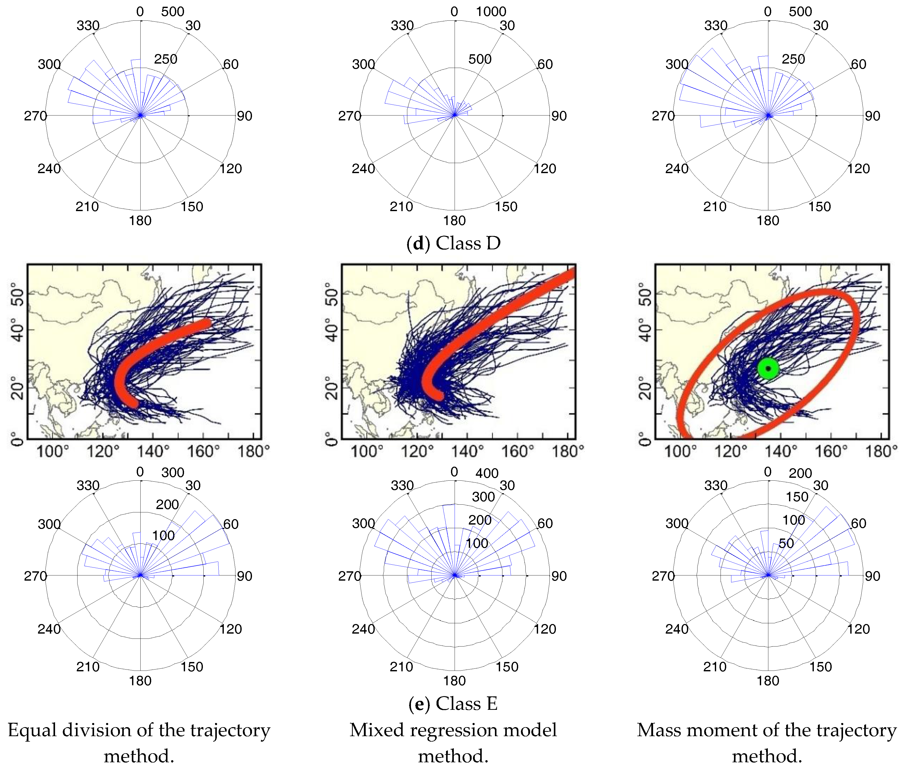
3.2. Trajectory Features of Different TC Classes

Figure 3 shows the TC trajectories contained in the different classes and the corresponding class centres. The clustering results for the same group obtained by the different clustering algorithms are placed on the same row, and the corresponding frequency distribution of the heading of TC trajectories in the class is shown at the lower part. This frequency, which reveals the heading distribution of TC movement at a 10° interval, is an accumulation of the angle between any two adjacent points in the TC trajectory.

The TC tracks in classes A, B, and C are primarily in found a straight westward movement. From the perspective of spatial distribution, these straight-moving classes are primarily distributed in the region to the south of 30° N. Class A is primarily concentrated in the region of the SCS, i.e., the trajectories were generated locally in the SCS. The trajectories contained in class B and class C represent TCs generated in the WNP that move into the SCS. The heading frequencies for these three categories show obvious single-peak distribution and are primarily distributed in the range near 280°. In addition, different clustering algorithms show relatively high consistency in their clustering results.

The class centre curve pattern for class D and class E show that these two classes are re-curving TC classes: TCs in these two classes move to high latitudes after turning near the SCS. The overall movement distances of the trajectories in class E are greater, reaching approximately 60° N. In addition, these two classes both have a relatively large spatial distribution range. Moreover, the frequency distributions of heading for these two classes are the double-peak distributions in the northwest and northeast direction. However, the heading frequency distribution of trajectories in class D (middle of Figure 3d) obtained by the mixed regression model shows a significant single-peak structure moving in the northwest direction. In contrast, the results obtained by the equal division of the trajectory method and mass moment of the trajectory method have two obvious peaks in the northwest and northeast directions, indicating that for class D, obtained by the mixed regression model, western movement is the predominant moving trend for TCs, although the class centre curve pattern shows a northward re-curving motion pattern.

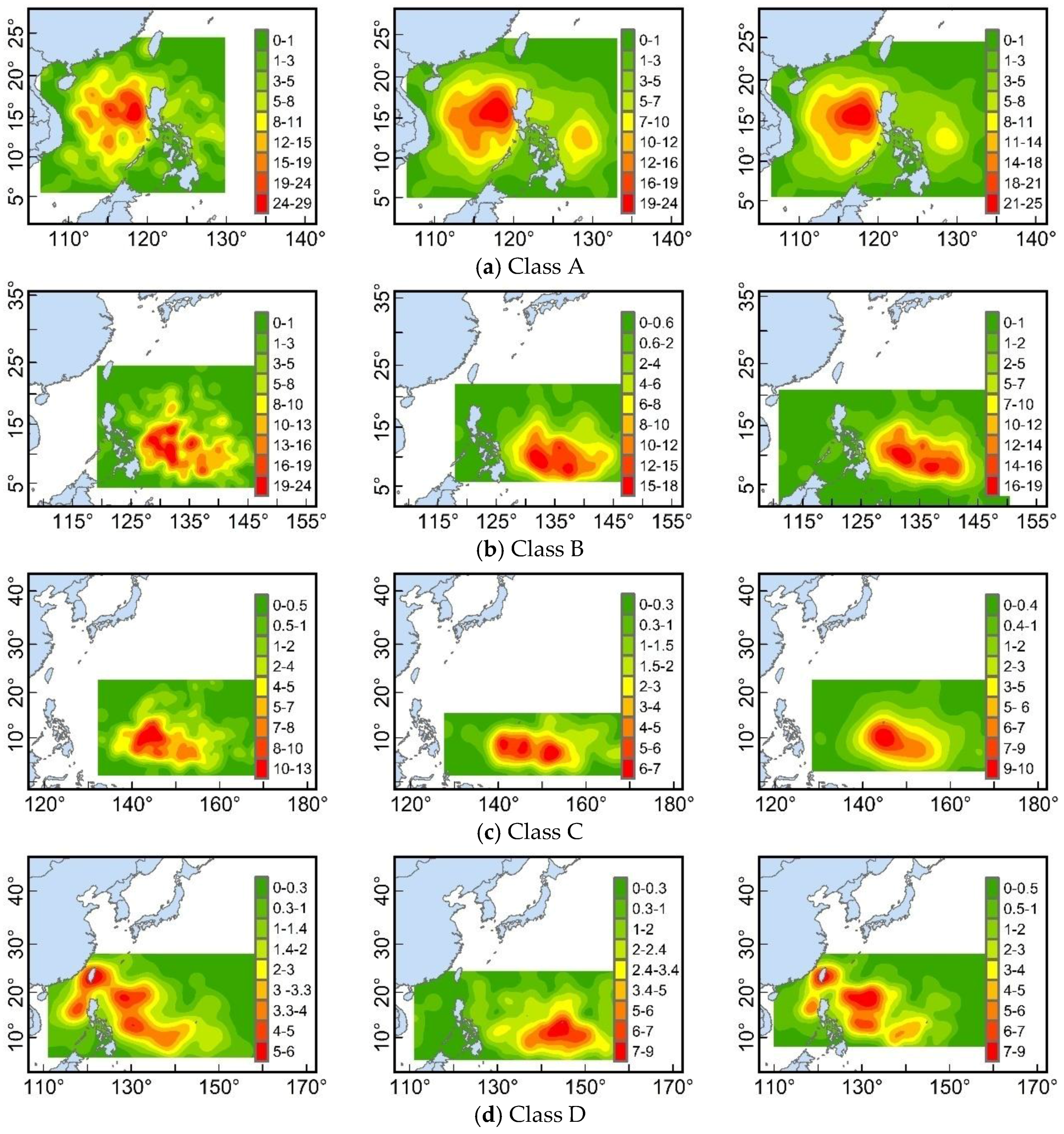
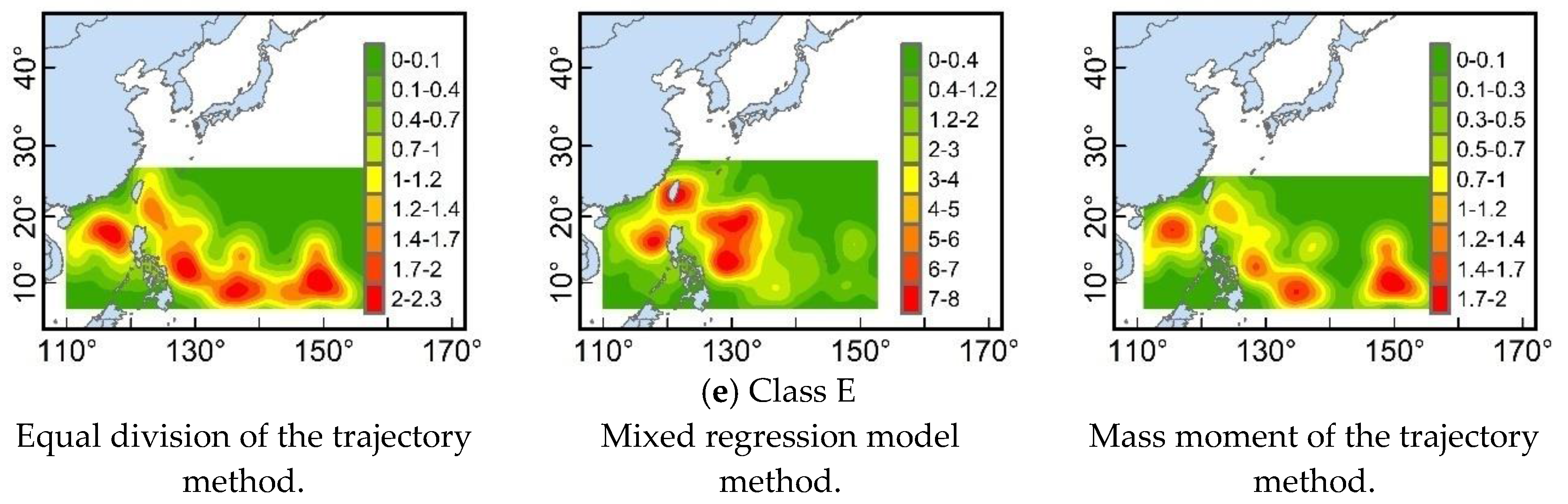
3.3. Genesis Locations of Different TC Classes

The spatial location of TC generation is connected—to a certain extent—to the movement mode of its trajectory [11]. It can be seen from the kernel density distribution (KDE) of the genesis positions (Figure 4) that the spatial distribution of TC genesis locations for three westward straight-moving classes (classes A, B, and C) obtained through different methods are essentially consistent (Figure 4a–c). The average longitudes for the genesis locations of classes A, B, and C are approximately 118° E, 135° E, and 150° E, respectively (

Table 3. Average longitude and latitude coordinates of the starting TC trajectory points in different classes.

TC Trajectory Class	Equal Division of the Trajectory Method		Mixed Regression Model Method		Mass Moment of the Trajectory Method
	Longitude	Latitude	Longitude	Latitude	Longitude	Latitude
Class A	117.38	14.914	118.99	14.47	118.90	14.72
Class B	134.01	11.81	135.94	10.79	135.09	10.28
Class C	148.93	9.78	150.84	7.87	150.04	9.62
Class D	130.67	16.06	142.38	12.43	130.66	17.00
Class E	132.75	13.75	127.75	17.05	132.96	13.89

), which corresponds to the three major source regions for TC generation in the WNP, namely, the SCS basin, the Philippine Basin, and the Mariana Islands [46], respectively.

However, for the TC trajectories in classes D and E, considerable differences are observed. Figure 4d shows that the spatial distribution of TC genesis locations for class D obtained by the equal division of the trajectory method and mass moment of the trajectory method is relatively scattered and primarily restricted to the west of 140° E, with the main concentration in the Philippine Basin, the SCS, and the area around Taiwan Island. Moreover, the average longitude for the genesis locations is located near 130° E (Table 3). In contrast, for class D obtained by the mixed regression model method, the TC genesis location is more concentrated and primarily distributes to the east of 140 °E, near the region of the Mariana Islands. According to the previous analyses, the class D obtained by the mixed regression model method is a mixed cluster, containing both straight and re-curving TC trajectories forming to the east of 140° E, and shows a significant west-moving trend Figure 3d). Compared with class C obtained by the mixed regression model method, which is also a class that primarily contains west straight-moving TC trajectories forming to the east of 140° E, the main difference is that the average latitude of TC genesis positions in class D are located in a more northerly position, located at approximately 12° N. Class C is located at approximately 7° N (Table 3). Therefore, classes C and D obtained by the mixed regression model generate a division of western-moving TCs based on latitude difference, which leads to the member TCs in class C obtained by the mixed regression model method representing only 13% of the overall number of TCs, relatively less than the results obtained by the other two methods (Table 2).

The spatial distributions of TC genesis locations in class E (to the left and right of Figure 4e) obtained by the equal division of the trajectory and the mass moment of the trajectory methods are more dispersive, and they are widely distributed from the SCS to 150° E. This means that TCs in this class present shapes that are more similar in trajectory than the genesis positions. In comparison, class E (seen in the middle of Figure 4e) obtained by the mixed regression mode shows more consistency in spatial distribution of TC genesis positions and is relatively similar to that of class D (seen on the left and right of Figure 4d) obtained by the equal division of the trajectory method and the mass moment of the trajectory method.

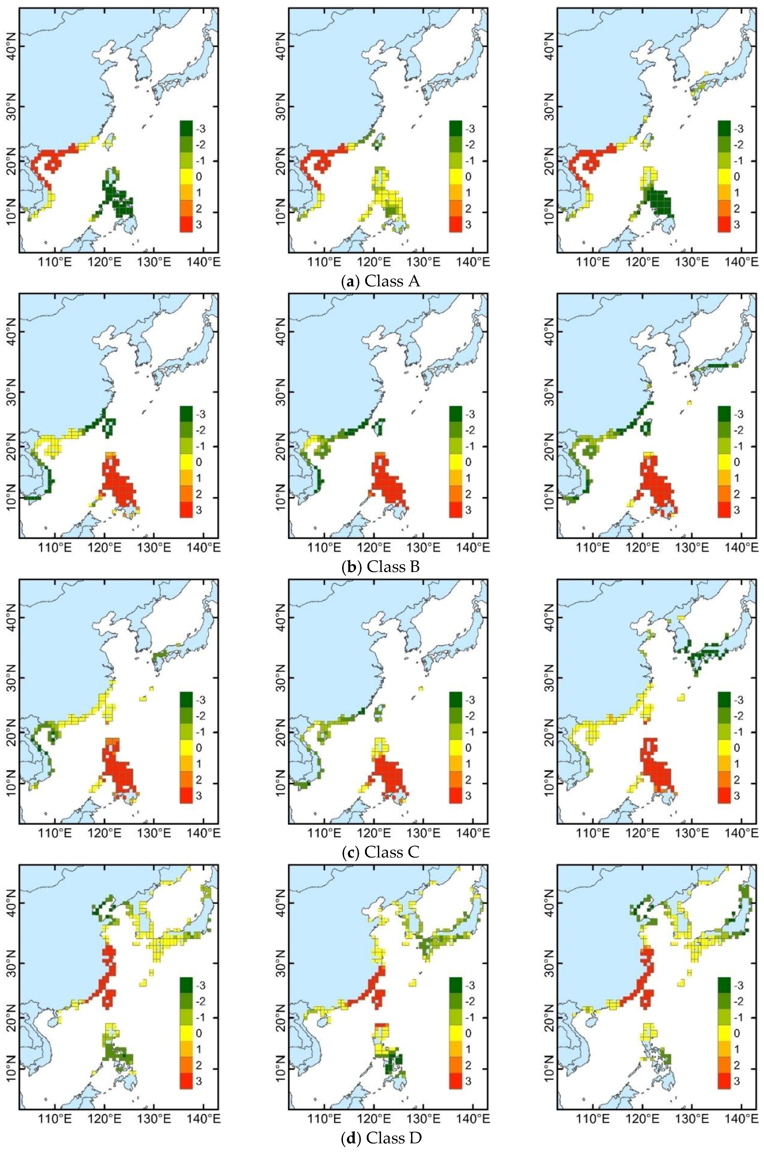
3.4. Landfall Locations for Different TC Classes

Landfall locations are directly associated with TC disasters. Therefore, to obtain a better understanding for landfall rules of TCs in different classes, a hot-spot analysis of landfall locations was performed for different TC categories. The analysis identified statistically significant spatial clusters of hot spots and cold spots, which correspond to frequent landfall locations and infrequent landfall locations, respectively. The analytical results are shown in Figure 5. In the figure, the red areas indicate frequent landfall locations, and the green areas indicate infrequent landfall locations. Figure 5 shows that the frequent landfall locations for different classes of TCs can be divided into two types. The frequent landfall locations for westward straight-moving TCs are the surrounding countries and regions of the SCS to the south of 22° N. The frequent landfall locations for northward re-curving TCs are located in the eastern coastal region of China to the north of 22° N.

From the perspective of different trajectory categories, for TCs in class A (Figure 5a), the frequent landfall locations are primarily concentrated in the coastal regions of South China and the northern region of Vietnam. The Philippines is an obvious infrequent landfall location. For TCs in classes B (Figure 5b) and C (Figure 5c), the most obvious frequent landfall locations are concentrated along the coast of the Philippines; the coastal regions of South China and Vietnam are comparatively infrequent landfall locations. Compared to the average latitude of the genesis location of TCs in class C obtained by the equal division of the trajectory and the mass moment of the trajectory methods, the class C genesis location obtained by the mixed regression model is located in a more southerly position (Table 3), and therefore, it does not form a significant frequent landfall location in the north of Luzon Island, unlike class C obtained by the other two methods.

The frequent landfall location for class D is mainly concentrated in the eastern and southeastern areas of China. Because class D obtained by the mixed regression model is a mixed TC trajectory class with a dominant westward heading, the frequent landfall location for this class occurs more to the south, extending only to Zhejiang Province in China (in the middle of Figure 5d). In contrast, the frequent landfall location of class D obtained by the other two trajectory clustering algorithms extends further northward and reaches Jiangsu Province of China (on the left and right of Figure 5d).

The frequent landfall location of class E obtained by the mixed regression model (in the middle of Figure 5e) is consistent with that of class D obtained by the equal division of the trajectory and the mass moment of the trajectory methods (on the left and right of Figure 5d) for their similarity in TC trajectory shape and genesis position, as mentioned in the previous section. However, class E obtained by the equal division of the trajectory and mass moment of the trajectory methods forms only a finite frequent landfall location in the eastern coast region of China.

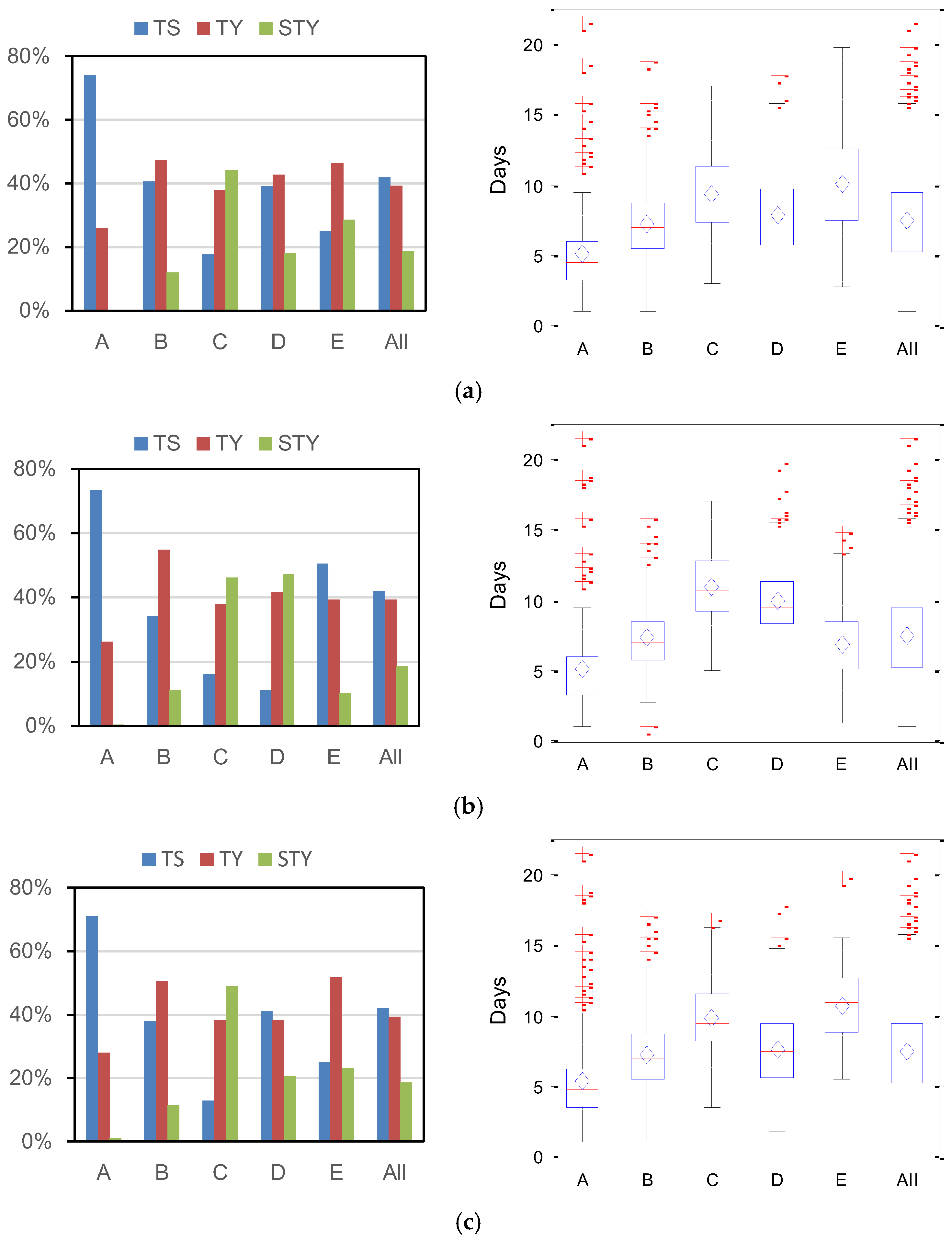
3.5. Intensity and Lifetime of Different TC Classes

The distribution of maximum intensity levels reached by the TCs in the various classes over the lifetime of the TC is shown in Figure 6. TCs are categorized into tropical storm (TS, 17.2 $\le v_{max}\le$ 32.6 m/s), typhoon (TY, 32.7 $\le v_{max}\le$ 50.9 m/s) and super typhoon (STY, $v_{max}\ge$ 51.0 m/s) categories according to their grade of maximum wind. For all the TCs shown in Figure 6, the proportion of tropical storms and typhoons is essentially the same: both account for approximately 40% of the overall TCs. The proportion of TCs reaching the level of super typhoon is approximately 20%.

There are some differences in the intensity distribution of TCs in different classes. Among these results, relatively high consistency in the intensity distribution tendency of TCs can be seen in the clustering results obtained by the equal division of the trajectory method (Figure 6a) and the mass moment of the trajectory method (Figure 6c). The maximum intensity level of the TCs in class A is relatively low because of the limited spatial scale of the SCS basin and the influence of the surrounding land. The tropical storm type accounts for the vast majority (>70%) of the TCs in class A, followed by the typhoon level, which accounts for approximately 26%; however, few super-typhoon TCs are observed in this class. The TCs in classes B and D are similar, and the proportion of tropical storm and typhoon-level TCs is essentially the same and comprises the vast majority of TCs (>80%) in the classes. A few super-typhoon TCs occur in classes B and D.

In class C, the super-typhoon TCs and typhoon TCs account for the vast majority (>80%). One significant difference is that the proportion of super-typhoon TCs in this class exceeds the proportion of the other two types of TCs, accounting for more than 40%. The TCs in class C have longer moving distances and lifetimes in general because of their easternmost genesis regions near the Mariana Islands (on the right side of Figure 6a); therefore, these TCs are more likely to reach higher intensities [47,48,49]. The opposite situation is true for TCs in class A, which have the shortest lifetime and lowest strength distribution.

The average lifetime is longest for class E TCs. Therefore, TCs in this class also have a relatively strong intensity. The proportion of TCs reaching typhoon intensity is approximately 50%, and the proportion of super typhoons exceeds 20%. The proportion of super typhoons that is relatively lower than class C may be related to the re-curving north movement of TCs in class E, where cooler sea surface temperature inhibits the development of intense TCs [50].

For TCs in classes obtained by the mixed regression model (Figure 6b), the intensity statistical results exhibit different features. The intensity of TCs in class D also have the highest proportion of strong TC intensity, similar to that of TCs in class C. This is an embodiment of the similarity of TCs in intensity distribution in these two classes, which show a relatively high consistency in the trajectory movement trend and genesis position. The lifetime statistics show that the TCs in class D are the second-longest (on the right of Figure 6b) among the TC groups obtained by the mixed regression model. The northward re-curving TCs in class E show similarity in intensity distribution and lifetime to those in class D obtained by the equal division of the trajectory and the mass moment of the trajectory methods. Both of these classes have main genesis locations restricted to the west of 140 °E concentrated in the Philippine Basin and the SCS. The tropical storm and typhoon-level TCs comprise the vast majority (~90%), and the average lifetime is approximately seven days, which is close to the total average value.

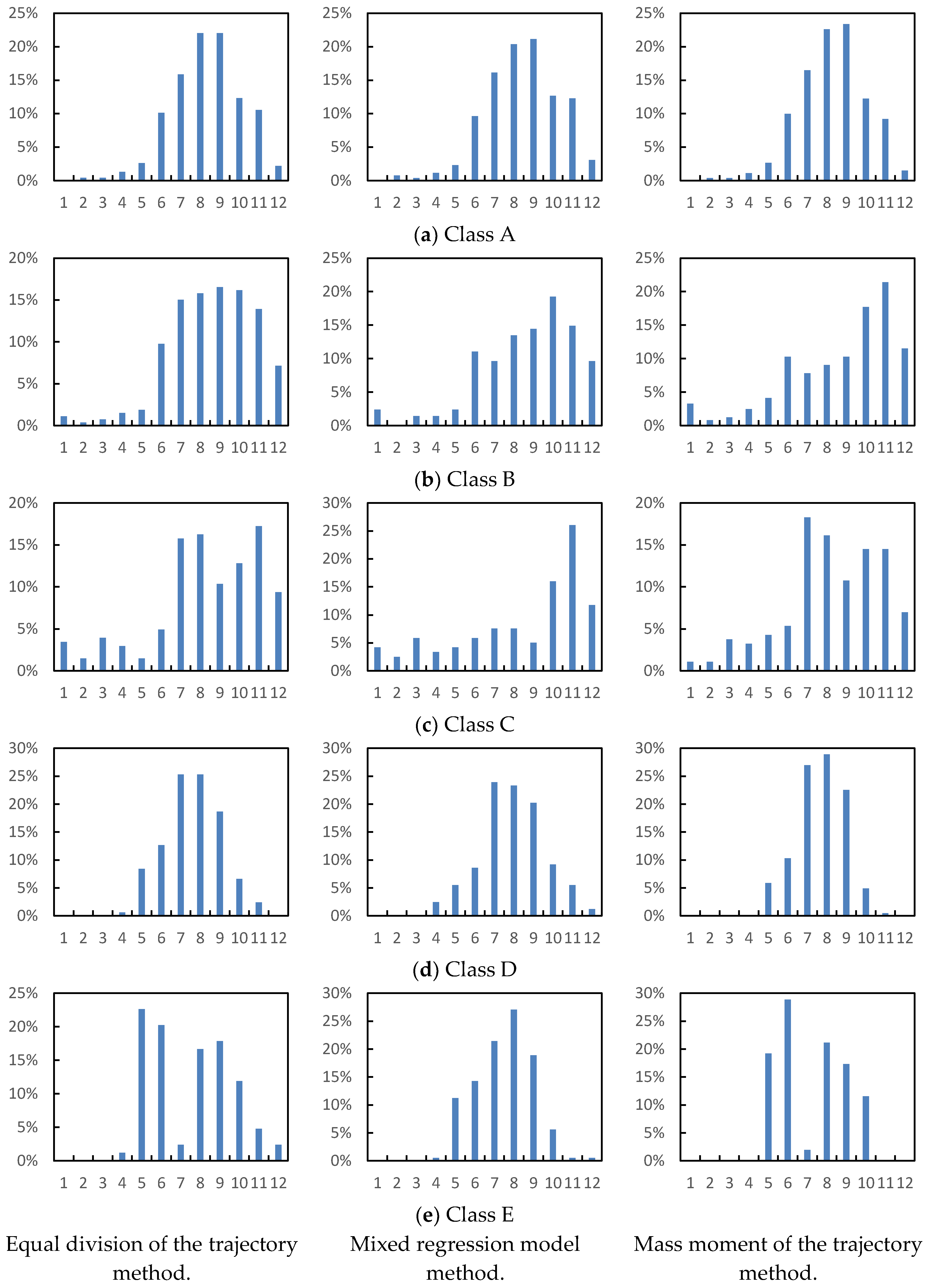
3.6. Seasonal Distribution of Different TC Classes

The seasonal distribution for class A (Figure 7a) is primarily concentrated in June–November, and relatively high consistency is reached for the results obtained by the different algorithms for this class. TCs in class B obtained by the equal division of the trajectory method (on the left of Figure 7b) are primarily distributed from July–November. The relatively larger spread time is likely related to the relatively high sea surface temperature of the Philippine Sea, which are higher than 26 °C [30]. In contrast, for class B obtained by the mass moment of the trajectory method (on the right of Figure 7b), more TC activities are observed for October–November. The average genesis position statistic results show that TCs in class B obtained by the mass moment of the trajectory method are located in a relatively more southerly location than those obtained by the equal division of the trajectory method (Table 3). This reflects that the average generation position of TCs in the WNP gradually moves northward from June to August and begins to retreat southward beginning in September [6,51].

For the TCs in class C obtained by the equal division of the trajectory and the mass moment of the trajectory methods, the seasonal distribution has obvious double peaks in July, August, October and November (left and right of Figure 7 c). This distribution follows the straight-moving TCs, which are mostly distributed in the early and late stages of the TC season in the WNP [6,51]. The northward re-curving moving trajectory of class D is primarily concentrated during July-September (on the left and right of Figure 7d). Although class D obtained by the mixed regression model method has a similar form of seasonal distribution (in the middle of Figure 7d), it is important to remember that this class is a mixture class and contains numerous westward straight-moving TC trajectories. Compared to the genesis position with class C, which was also obtained by the mixed regression model method, TCs in class C shifted more southward (Table 3). In addition, the seasonal distribution of class C displays a pronounced winter active mode concentrated in October-December (in the middle of Figure 7c). Accordingly, these two classes obtained by the mixed regression model method together also reflect the north-south oscillation of the genesis positions of TCs with the change of seasonality in the WNP.

The seasonality distribution of TC activity in class E (on the left and right of Figure 7e) exhibits a bimodal pattern and is concentrated during the conversion from spring to summer and summer to fall in May, June, August, September, and October. This seasonal distribution reflects the seasonal distribution of the extratropical transition of TC in the WNP, which is related to large-scale circulation modes and high-altitude trough activity in the mid-high latitude region over the WNP [52,53]. The statistical analysis indicates that 82% of the TCs in class E obtained by the equal division of the trajectory method experienced an extratropical transition process, and 94% of the TCs in the class obtained by the mass moment of the trajectory method experienced an extratropical transition process. The seasonal distribution of class E obtained by the mixed regression model method has more similarity to that of class D obtained by the equal division of the trajectory method and the mass moment of the trajectory method. This result is consistent with the similarity of class features for these classes as analysed previously.

4. Discussion

In this paper, three clustering methods were applied to analyse the trajectory of TCs that affect the SCS. Among these methods, the equal division of the trajectory method and the mass moment of the trajectory method preprocess the original trajectory data into a structure that can express the characteristics of the original trajectory and satisfy the data-processing requirements of normal clustering algorithms. In contrast, the mixed regression model method can conduct clustering operations on the original trajectory data with different lengths based on a special mathematical regression model.

The form of the clustering centre provides a preliminary understanding of the overall characteristics of the elements in the class. The TC cluster centre obtained by different methods are different (Figure 2). Among these cluster centres, the mass moment of the trajectory method obtains a variance ellipse class centre, which provides a good expression of the spatial distribution of the trajectory. Both the equal division of the trajectory method and the mixed regression model method acquired a line-type class centre. However, the class centre for the mixed regression model still produced curve lines in the cases of classes A and B (Figure 2b), even though these classes primarily consist of straight-moving TC trajectories. This observation produces a confusing expression for the TC trajectory mode of the classes. However, the class centres acquired by the equal division of the trajectory method provide a relatively simple and clear expression (Figure 2a) corresponding to the TC trajectory mode of classes A and B. The reason may be that the mixed regression model method is essentially based on a quadratic polynomial curve fitting process, which may be more susceptible to the effect of abnormal trajectories in the class. Thus, the cluster centre takes the form of a curve, and it cannot accurately reflect the overall characteristics of TC trajectories in the class. In contrast, the class centre obtained by the equal division of the trajectory method is a result of an averaging operation of all TC trajectory data in the class. Therefore, the influences of abnormal trajectories in the class are eliminated by the averaging process. In addition, the cluster centre can better embody the overall tendency of the moving trend of TCs in the class.

The previous analysis shows that differences are observed in the results obtained from the different models. These differences reflect the methods’ individual features.

Table 4. Comparison of three clustering methods for the trajectory.

Clustering Method	Equal Division of the Trajectory Method	Mixed Regression Model Method	Mass Moment of the Trajectory Method
Type of method	Combination with the general clustering model after the transformation of the original trajectory	Cluster the original trajectory data based on the mathematical model	Combination with the general clustering model after the transformation of the original trajectory
Model complexity	Simple	Complicated	Relatively complicated
Information contained	Spatial location and shape information of the trajectory	Original complete trajectory information	Spatial location, shape information and some velocity information of the trajectory
Clustering results	Trajectory shape consistency is relatively good	Trajectory spatial consistency is relatively good	Essentially similar to the equal divide method
Class centre	Average trajectory in the class	Quadratic curve	Variance ellipse

summarizes the main characteristics of the different algorithms. For the equal division of the trajectory method, the velocity information contained in the original trajectory cannot be retained after the equal division of the trajectory is performed. The mass moment of the trajectory method retains the velocity information of the original trajectory, at least to an extent. However, this transformation process also produces biases in the space and shape information expression of the TC trajectory and may induce some deviation in the clustering result. Figure 8 shows a re-curving trajectory mixed in the straight-moving trajectory class C obtained by the mass moment of the trajectory method. The left side of the figure shows the original observation points of the TC trajectory, and the right side is the equal division point of the trajectory. It can be seen from Figure 8a that when the TC moved to a high latitude, the accelerated velocity caused a decrease in the number of observation data points in the trajectory obtained in the same time interval; therefore, the central point of the trajectory is more to the south and closer to the side of the trajectory with dense sampling points. In addition, the long axis direction of the variance ellipse is consistent with the distribution direction of the dense trajectory points. In Figure 8b, because the equal division sampling points are uniformly distributed, the central point is shifted to the north, closer to the geometric centre of the trajectory, and the variance ellipse indicates the overall distribution trend of the trajectory. Therefore, the central point and the variance ellipse are more susceptible to the sample points in the trajectory, which may influence the clustering result and result in some mixture of trajectory types in the TC trajectory cluster. However, the overall clustering results show that, for TC trajectory, it is not the velocity but the shape and spatial location that are the main factors in determining the clustering results. This finding is consistent with the previous view [6,30]. Moreover, in comparison, relatively high consistency is observed for the clustering results obtained by the mass moment of the trajectory method and the equal division of the trajectory method.

The mixed regression model method has a solid theoretical mathematical basis. The clustering operation can be conducted for the original trajectory data without preprocessing. By expanding the dimension of the polynomial coefficient matrix, this method can conveniently add variable factors that are likely to play a role in clustering results into the model. Through regression fitting, the clustering results show relatively good concentration for the TC spatial location. However, the quadratic polynomial used to fit the TC trajectory will likely cause a mixture of the various types of TC trajectory. Figure 9 shows the quadratic polynomial fitting of the TC trajectories with different movements contained in class D according to the mixed regression model method. The red trajectory represents the fitted quadratic polynomial curve. For the straight trajectory and the re-curving trajectory with relatively high local similarity, we can achieve a relatively good fit through the same quadratic polynomial curve.

To compare the trajectory motion modes in the clustering results obtained by the various algorithms, cosine similarity statistics between the trajectories in the different classes were conducted (

Table 5. Cosine similarity statistics of TC trajectories in different classes obtained by the various trajectory clustering methods.

Clustering Method	Equal Division of the Trajectory Method			Mixed Regression Model Method			Mass Moment of the Trajectory Method
	Mean	Maximum	Minimum	Mean	Maximum	Minimum	Mean	Maximum	Minimum
Class A	0.991	1.000	0.914	0.990	1.000	0.924	0.991	1.000	0.914
Class B	0.993	1.000	0.944	0.994	1.000	0.963	0.992	1.000	0.928
Class C	0.992 *	1.000	0.950	0.991 *	1.000	0.939	0.986	1.000	0.898
Class D	0.988	1.000	0.911	0.981	1.000	0.877	0.986	1.000	0.922
Class E	0.987 *	1.000	0.940	0.982	1.000	0.885	0.987 *	1.000	0.940

Note: The asterisk * indicates the difference is not significant at the 0.05 level.

). The statistical results show that, in general, the algorithms all obtain relatively good TC trajectory clustering results. The results of the equal division of the trajectory method are more consistent in TC trajectory movement, especially for the re-curving trajectories in classes D and E. The average cosine similarities of these two classes are 0.988 and 0.987 for the equal division of the trajectory method. For the mixed regression model method, the similarities are 0.981 and 0.982, which are the lowest among these three methods. The statistical results are significant at the 0.05 level.

The above analyses suggest that the equal division of the trajectory method provides a simple and direct solution to the problem. This algorithm also reaches a relatively better clustering result from the standpoint of the characteristic expression and consistency of the TC trajectory movement in the class. For the mass moment of the trajectory method, the spatial distribution of TC trajectories in different classes is well displayed through a variance ellipse form class centre. It may be somewhat difficult to select the proper length of the clutter centre for the mixed regression model method to more accurately express the characteristics of TC tracks in the class. A relatively greater mixture of different types of TC trajectories may be caused in the clustering result. However, a relatively high spatial concentration of TC trajectories in the clustering result is achieved with this algorithm, which may be a priority option in the case of TC trajectory spatial consistency being retained.

5. Conclusions

In this article, three trajectory clustering algorithms were applied to analyse the trajectories of TCs that affected the SCS from 1949 to 2014. Based on the complete spatial position and trajectory shape information of the TC trajectories, five trajectory clusters were obtained, including three western straight-line movement trajectory clusters and two northward re-curving trajectory clusters.

The TC trajectories in different clusters show different characteristics in their properties, such as lifetime, strength, movement distance, landfall location, and seasonality distribution. For the TCs in class A, which were generated in the most western region, within the SCS, the intensity is weaker overall. The TCs in class C, which were generated in the most eastern region at approximately 145 °E near the Mariana Islands, have the highest proportion of super-typhoon grade TCs for their longer movement distance and extended lifetimes. The landfall location analysis shows that the northward re-curving TCs were primarily concentrated along the coasts of the eastern provinces of China. Two landfall types are observed for the westward straight-moving TCs. For the TCs in class A, the landfall locations were primarily concentrated in the coastal regions of South China and north of Vietnam. For the TCs from the WNP in classes B and C, the most affected area was the Philippines.

The monthly activity frequency distribution of TCs in classes A and B were primarily distributed during June–November. There are no obvious peak seasons for the TCs generated east of the Philippines in class B. For the TCs in class C, two obvious peak seasons are observed in the early and late stages of the TC season. The northward re-curving TCs in class D are primarily concentrated in the period from July–September. In contrast, the TCs in class E obtained by the equal division of the trajectory and the mass moment of the trajectory methods are primarily concentrated during the conversion from spring to summer and summer to fall, reflecting the seasonality distribution characteristics of TCs experiencing extratropical transition.

A comparison of the results obtained by these trajectory-clustering algorithms shows that the equal division of the trajectory method provide a better clustering result generally. The class centre provides a simple and clear expression for the pattern of TC tracks in the class. In addition, the heading of TC tracks maintains a relatively good consistency in the class. The results obtained by the trajectory mass moment algorithm are more consistent with the results obtained by the equal division of the trajectory method. The mixed regression model method, which presents higher sensitivity in the trajectory position, can obtain TC clusters with a more concentrated spatial distribution.

References

1. Wang, Y.; Wu, C.-C. Current understanding of tropical cyclone structure and intensity changes—A review. Meteorol. Atmos. Phys. 2004, 87, 257–278. [Google Scholar] [CrossRef]
2. Chan, J.C.L.; Liu, K.S.; Ching, S.E.; Lai, E.S.T. Asymmetric distribution of convection associated with tropical cyclones making landfall along the South China Coast. Mon. Weather Rev. 2004, 132, 2410–2420. [Google Scholar] [CrossRef]
3. McGregor, G.R. The tropical cyclone hazard over the South China Sea 1970–1989. Appl. Geogr. 1995, 15, 35–52. [Google Scholar] [CrossRef]
4. Gemmer, M.; Yin, Y.; Luo, Y.; Fischer, T. Tropical cyclones in China: County-based analysis of landfalls and economic losses in Fujian Province. Quat. Int. 2011, 244, 169–177. [Google Scholar] [CrossRef]
5. Li, X.; Ren, F.; Yang, X.; Wang, C. A study of the regional differences of the tropical cyclone activities over the South China Sea and the Western North Pacific. Clim. Environ. Res. 2010, 15, 504–510. (In Chinese) [Google Scholar]
6. Kim, H.S.; Kim, J.H.; Ho, C.H.; Chu, P.S. Pattern classification of typhoon tracks using the fuzzy c-means clustering method. J. Clim. 2011, 24, 488–508. [Google Scholar] [CrossRef]
7. Saunders, M.A.; Chandler, R.E.; Merchant, C.J.; Roberts, F.P. Atlantic hurricanes and NW Pacific typhoons: ENSO spatial impacts on occurrence and landfall. Geophys. Res. Lett. 2000, 27, 1147–1150. [Google Scholar] [CrossRef]
8. Wang, B.; Chan, J.C.L. How strong ENSO events affect tropical storm activity over the western north Pacific. J. Clim. 2002, 15, 1643–1658. [Google Scholar] [CrossRef]
9. Hodanish, S.; Gray, W.M. An observational analysis of tropical cyclone recurvature. Mon. Weather Rev. 1993, 121, 2665–2689. [Google Scholar] [CrossRef]
10. Elsner, J.B.; Liu, K.-B. Examining the ENSO-typhoon hypothesis. Clim. Res. 2003, 25, 43–54. [Google Scholar] [CrossRef]
11. Harr, P.A.; Elsberry, R.L. Tropical cyclone track characteristics as a function of large-scale circulation anomalies. Mon. Weather Rev. 1991, 119, 1448–1468. [Google Scholar] [CrossRef]
12. Harr, P.A.; Elsberry, R.L. Large-scale circulation variability over the tropical western north Pacific. Part I: Spatial patterns and tropical cyclone characteristics. Mon. Weather Rev. 1995, 123, 1225–1246. [Google Scholar] [CrossRef]
13. Harr, P.A.; Elsberry, R.L. Large-scale circulation variability over the tropical western north Pacific. Part II: Persistence and transition characteristics. Mon. Weather Rev. 1995, 123, 1247–1268. [Google Scholar] [CrossRef]
14. Lander, M.A. Specific tropical cyclone track types and unusual tropical cyclone motions associated with a reverse-oriented monsoon trough in the western North Pacific. Weather Forecast. 1996, 11, 170–186. [Google Scholar] [CrossRef]
15. Liu, K.; Chan, J.C. Climatological characteristics and seasonal forecasting of tropical cyclones making landfall along the South China coast. Mon. Weather Rev. 2003, 131, 1650–1662. [Google Scholar] [CrossRef]
16. Li, Y.; Chen, L.-S.; Zhang, S.-J. Statistical characteristics of tropical cyclone making landfalls on China. J. Trop. Meteorol. 2004, 20, 14–23. (In Chinese) [Google Scholar]
17. Liu, X.; Ban, Y. Uncovering spatio-temporal cluster patterns using massive floating car data. ISPRS Int. J. Geo-Inf. 2013, 2, 371–384. [Google Scholar] [CrossRef]
18. Qiu, J.; Wang, R. Road map inference: A segmentation and grouping framework. ISPRS Int. J. Geo-Inf. 2016, 5, 130. [Google Scholar] [CrossRef]
19. Shi, Y.; Deng, M.; Yang, X.; Liu, Q.; Zhao, L.; Lu, C.-T. A framework for discovering evolving domain related spatio-temporal patterns in Twitter. ISPRS Int. J. Geo-Inf. 2016, 5, 193. [Google Scholar] [CrossRef]
20. Markman, V. Unsupervised discovery of fine-grained topic clusters in Twitter posts. In Proceedings of the Analyzing Microtext: Papers from the 2011 AAAI Workshop, San Francisco, CA, USA, 8 August 2011. [Google Scholar]
21. Sun, Y.; Fan, H.; Li, M.; Zipf, A. Identifying the city center using human travel flows generated from location-based social networking data. Environ. Plan. B Plan. Des. 2016, 43, 480–498. [Google Scholar] [CrossRef]
22. Sârbu, C.; Einax, J.W. Study of traffic-emitted lead pollution of soil and plants using different fuzzy clustering algorithms. Anal. Bioanal. Chem. 2008, 390, 1293–1301. [Google Scholar] [CrossRef] [PubMed]
23. Chen, J.-C.; Lin, K.-Y. Diagnosis for monitoring system of municipal solid waste incineration plant. Expert Syst. Appl. 2008, 34, 247–255. [Google Scholar] [CrossRef]
24. Cheng, S.Y.; Wang, F.; Li, J.B.; Chen, D.S.; Li, M.J.; Zhou, Y.; Ren, Z.H. Application of Trajectory Clustering and Source Apportionment Methods for Investigating Trans-Boundary Atmospheric PM10 Pollution. Aerosol Air Qual. Res. 2013, 13, 333–342. [Google Scholar] [CrossRef]
25. MacQueen, J. Some methods for classification and analysis of multivariate observations. In Proceedings of the Fifth Berkeley Symposium on Mathematical Statistics and Probability; University of California Press: Berkely, CA, USA, 1967; pp. 281–297. [Google Scholar]
26. Elsner, J.B. Tracking hurricanes. Bull. Am. Meteorol. Soc. 2003, 84, 353–356. [Google Scholar] [CrossRef]
27. Blender, R.; Fraedrich, K.; Lunkeit, F. Identification of cyclone-track regimes in the North Atlantic. Q. J. R. Meteorol. Soc. 1997, 123, 727–741. [Google Scholar] [CrossRef]
28. Corporal-Lodangco, I.; Leslie, L. Cluster analysis of Philippine tropical cyclone climatology: Applications to forecasting. J. Climatol. Weather Forecast. 2016, 4, 2. [Google Scholar] [CrossRef]
29. Gaffney, J.S. Probabilistic Curve-Aligned Clustering and Prediction with Regression Mixture Models. Ph.D. Thesis, University of California, Oakland, CA, USA, 2004. [Google Scholar]
30. Camargo, S.J.; Robertson, A.W.; Gaffney, S.J.; Smyth, P.; Ghil, M. Cluster analysis of typhoon tracks. Part I: General properties. J. Clim. 2007, 20, 3635–3653. [Google Scholar] [CrossRef]
31. Gaffney, S.; Smyth, P. Trajectory clustering with mixtures of regression models. In Proceedings of the Fifth ACM SIGKDD International Conference on Knowledge Discovery and Data Mining, San Diego, CA, USA, 15–18 August 1999; pp. 63–72. [Google Scholar]
32. Camargo, S.J.; Robertson, A.W.; Gaffney, S.J.; Smyth, P.; Ghil, M. Cluster analysis of typhoon tracks. Part II: Large-scale circulation and ENSO. J. Clim. 2007, 20, 3654–3676. [Google Scholar] [CrossRef]
33. Kossin, J.P.; Camargo, S.J.; Sitkowski, M. Climate modulation of North Atlantic hurricane tracks. J. Clim. 2010, 23, 3057–3076. [Google Scholar] [CrossRef]
34. Nakamura, J.; Lall, U.; Kushnir, Y.; Camargo, S.J. Classifying North Atlantic tropical cyclone tracks by mass moments. J. Clim. 2009, 22, 5481–5494. [Google Scholar] [CrossRef]
35. Camargo, S.J.; Robertson, A.W.; Barnston, A.G.; Ghil, M. Clustering of Eastern North Pacific tropical cyclone tracks: ENSO and MJO effects. Geochem. Geophys. Geosyst. 2008, 9. [Google Scholar] [CrossRef]
36. Paliwal, M.; Patwardhan, A. Identification of clusters in tropical cyclone tracks of North Indian Ocean. Nat. Hazards 2013, 68, 645–656. [Google Scholar] [CrossRef]
37. Yang, L.; Du, Y.; Wang, D.; Wang, C.; Wang, X. Impact of intraseasonal oscillation on the tropical cyclone track in the South China Sea. Clim. Dyn. 2014, 44, 1505–1519. [Google Scholar] [CrossRef]
38. Goh, A.Z.-C.; Chan, J.C.L. Interannual and interdecadal variations of tropical cyclone activity in the South China Sea. Int. J. Climatol. 2010, 30, 827–843. [Google Scholar] [CrossRef]
39. Ying, M.; Zhang, W.; Yu, H.; Lu, X.; Feng, J.; Fan, Y.; Zhu, Y.; Chen, D. An Overview of the China Meteorological Administration Tropical Cyclone Database. J. Atmos. Ocean. Technol. 2014, 31, 287–301. [Google Scholar] [CrossRef]
40. Ren, F.; Liang, J.; Wu, G.; Dong, W.; Yang, X. Reliability Analysis of Climate Change of Tropical Cyclone Activity over the Western North Pacific. J. Clim. 2011, 24, 5887–5898. [Google Scholar] [CrossRef]
41. Chu, H.-J.; Liau, C.-J.; Lin, C.-H.; Su, B.-S. Integration of fuzzy cluster analysis and kernel density estimation for tracking typhoon trajectories in the Taiwan region. Expert Syst. Appl. 2012, 39, 9451–9457. [Google Scholar] [CrossRef]
42. Gaffney, S.J.; Robertson, A.W.; Smyth, P.; Camargo, S.J.; Ghil, M. Probabilistic clustering of extratropical cyclones using regression mixture models. Clim. Dyn. 2007, 29, 423–440. [Google Scholar] [CrossRef]
43. Davies, D.L.; Bouldin, D.W. A cluster separation measure. IEEE Trans. Pattern Anal. Mach. Intell. 1979, PAMI-1, 224–227. [Google Scholar] [CrossRef]
44. Bensaid, A.M.; Hall, L.O.; Bezdek, J.C.; Clarke, L.P.; Silbiger, M.L.; Arrington, J.A.; Murtagh, R.F. Validity-guided (re) clustering with applications to image segmentation. IEEE Trans. Fuzzy Syst. 1996, 4, 112–123. [Google Scholar] [CrossRef]
45. Abonyi, J.; Feil, B. Cluster Analysis for Data Mining and System Identification; Springer Science & Business Media: Berlin, Germany, 2007. [Google Scholar]
46. Chen, S.-R. Source regions of tropical Pacific storms over north west ocean. Meteorol. Mon. 1990, 16, 23–26. (In Chinese) [Google Scholar]
47. Camargo, S.J.; Sobel, A.H. Western North Pacific tropical cyclone intensity and ENSO. J. Clim. 2005, 18, 2996–3006. [Google Scholar] [CrossRef]
48. Chan, J.C. Decadal Variations of Intense Typhoon Occurrence in the Western North Pacific. In Proceedings of the Royal Society of London A: Mathematical, Physical and Engineering Sciences; The Royal Society: London, UK, 2008; pp. 249–272. [Google Scholar]
49. Mei, W.; Xie, S.-P.; Primeau, F.; McWilliams, J.C.; Pasquero, C. Northwestern Pacific typhoon intensity controlled by changes in ocean temperatures. Sci. Adv. 2015, 1, e1500014. [Google Scholar] [CrossRef] [PubMed]
50. Chen, L.; Ding, Y. An Introduction to Typhoons in the Northwest Pacific; Science Press Ltd.: Beijing, China, 1979; p. 491. (In Chinese) [Google Scholar]
51. Chia, H.H.; Ropelewski, C.F. The interannual variability in the genesis location of tropical cyclones in the northwest Pacific. J. Clim. 2002, 15, 2934–2944. [Google Scholar] [CrossRef]
52. Harr, P.A.; Elsberry, R.L.; Hogan, T.F. Extratropical transition of tropical cyclones over the western north Pacific. Part II: The impact of midlatitude circulation characteristics. Mon. Weather Rev. 2000, 128, 2634–2653. [Google Scholar] [CrossRef]
53. Zhong, Y.; Xu, M.; Wang, Y. Spatio-temporal distributive characteristics of extratropically transitioning tropical cyclones over the Northwest Pacific. Acta Meteorol. Sin. 2009, 67, 697–707. (In Chinese) [Google Scholar]
Figure 1. Variation of the coefficients of variation index with the number of clusters. The left side shows the result of the equal division of the trajectory method, and the right side is the result for the mass moment of the trajectory method. (a) Equal division of the trajectory method. (b) Mass moment of the trajectory method.
Ijgi 06 00210 g001
Figure 2. Clustering centres of the tropical cyclone (TC) trajectory obtained by different clustering algorithms: (a) clustering centre for the equal division of the trajectory method, (b) clustering centre for the mixed regression model method, and (c) clustering centre for the mass moment of the trajectory method.
Ijgi 06 00210 g002
Figure 3. (ae) TC trajectory clustering results and corresponding heading frequency distribution of TC movement obtained by the different trajectory clustering methods.
Ijgi 06 00210 g003aIjgi 06 00210 g003bIjgi 06 00210 g003c
Figure 4. (ae) kernel density distribution of genesis locations for the TC trajectories in the different classes according to the different trajectory clustering methods. The density is the number of TC genesis points per square kilometre, and the unit is 10−5 events /km2.
Ijgi 06 00210 g004aIjgi 06 00210 g004b
Figure 5. (ae) Spatial distribution of landfall locations for the TCs in different classes according to the different trajectory clustering methods. Red indicates the frequent landfall locations, and green indicates the infrequent landfall locations. A value of ±3 is statistically significant at a confidence level of 99%, ±2 is statistically significant at a confidence level of 95%, and ±1 is statistically significant at a confidence level of 90%; 0 indicates that the results are not significant.
Ijgi 06 00210 g005aIjgi 06 00210 g005b
Figure 6. The statistics of intensity distribution and lifetime of TCs in different classes obtained by the different trajectory clustering methods. The histograms on the left side of the figure show the intensity distribution of TCs in different classes; the corresponding boxplot on the right side shows the lifetime statistics of TCs in the classes. The line and the diamond within the box represent the median value and the mean value of the lifetime of TCs in the class, separately. (a) Intensity and lifetime statistical results obtained by equal division of the trajectory method; (b) Intensity and lifetime statistical results obtained by mixed regression model method; (c) Intensity and lifetime statistical results obtained by mass moment of the trajectory method.
Ijgi 06 00210 g006
Figure 7. (ae) Seasonal distributions of TCs in different classes according to the different trajectory clustering methods.
Ijgi 06 00210 g007
Figure 8. Central point and variance ellipse of the trajectory obtained by the (a) original trajectory points and (b) equal division trajectory points for Typhoon Emma (November 1959).
Ijgi 06 00210 g008
Figure 9. Quadratic polynomial fitting result of the TC trajectories.
Ijgi 06 00210 g009