Improving Identification of Areas for Ecological Restoration for Conservation by Integrating USLE and MCDA in a GIS-Environment: A Pilot Study in a Priority Region Northern Mexico

Abstract

Nature conservation is critical for securing an adequate supplying of environmental services to humans. Paradoxically, financial resources for conservation are normally scarce and, forest ecosystem restoration activities are expensive. So, a careful and detailed planning is vital for optimizing economic funds when ecosystems restoration practices are implemented. In this work, we developed a methodology to find physically-degraded sites in order to determine both, urgency and feasibility to carry out ecological forest restoration activities in the Priority Region for Conservation Xilitla in the state of San Luis Potosí (Mexico). Both, Universal Soil Loss Equation (USLE) and Multi-Criteria Decision Analysis (MCDA) were integrated together by using climatic, soil, remotely-sensed, and proximity data at a 30 m spatial resolution. The results indicated that, more than 80% of the bare soil land in the protected area is under several conditions that lead to feasible ecosystem restoration. This methodology can be further applied to know about the spatial location of soil degraded sites when planning forest restoration practices in natural protected areas.

1. Introduction

For centuries, soil has been affected by diverse environmental and anthropogenic factors, impacting significantly on its physical, chemical and biological properties, and placing it at some level of degradation [1,2,3]. Worldwide, more than 4.9 billion hectares (33%) have been affected by soil degradation processes [1]. In Mexico, during 1999, it was estimated that 95 million hectares (49% of the national territory) presented some kind of degradation in the soil, which increased to 125 million hectares (64%). Main causes of land degradation in Mexico by degree of occurrence are, urbanization with 57.6% , agricultural and livestock activities with 35%, and loss of vegetation cover with 7.4% [3].

There is an increasing interest in preventing, mitigating and reversing damage to ecosystems [4,5]. So, a number of approaches to prioritize sites requiring actions for conservation/restoration based on different considerations are reported i.e., carbon stock [6,7,8,9,10], sediment retention [11,12,13,14] and biodiversity [15,16,17]. In this sense, some approaches have been developed to prioritize areas for restoration focusing on protecting those places that are special, mainly due to a benefit they are providing. For example, some authors have focused on the watershed outcomes as environmental services as a measure to prioritize land for restoration. Legge [18] proposed an approach based on the outcomes generated by the watershed for prioritizing areas for restoration. They combined three models i.e., HIT, SWAT and WWAT (High Impact Target, Soil and Water Assessment Tool, Michigan’s Water Withdrawal Assessment Tool) and assigned the highest value to agricultural land where HIT model predicted high sediment loading, where WWAT estimated a low amount of groundwater as baseflow to streams, and on soils that would provide the highest groundwater recharge modeled in SWAT. Others have used the USLE model to prioritize watersheds that could have the more benefit in trapping sediment if would be restored [19]. For further reference on the objectives considered when prioritizing for restoration, they have been classified by targeting environmental benefits i.e., wildlife habitat, water quality, and water storage, among others [20].

When dealing with soil degradation, it is particularly important the focus on preventing it from soil erosion [14,21,22,23]. Particularly, the Universal Soil Loss Equation (USLE) allows estimating the annual soil loss due to water erosion, an important variable for the identification and planning actions, such as soil conservation and restoration practices. For example, Mohamed et al. [21] studied physicochemical soil degradation by determining erosion rate and salinity and sodicity levels as indicators of environmental risk in the northern coast of Egypt. Teshome et al. [22] used USLE to estimate erosion rates as indicators of effectiveness of soil and water conservation technologies in a mountainous region of Ethiopia. Meanwhile, others have applied the USLE model in a multi-temporal perspective to study dynamics of soil erosion rates through time. Meshesha et al. [14] estimated erosion change in a region of Ethiopia by using vegetation and land use data obtained from Landsat imagery for the years 1973, 1985 and 2006, and designed potential scenarios to evaluate the effectiveness of watershed management for controlling soil loss. While Mancino et al. [23] estimated soil loss (USLE) in a region of southern Italy (Matera prefecture) under a multitemporal approach (1960, 1990 and 2010). They considered land use as driving factor for diminishing erosion rates and supposed that land abandonment was the main cause of those changes. Further studies on temporal dynamics have investigated the impact of seasonality in estimating the C factor used in the USLE model, becoming particularly special when the focus of study is on intra annual variations of vegetation cover and its effect on soil erosion [24].

To prioritize soil degraded areas, by considering some factors that may favor or limit the applicability of ecological restoration activities, Multi-Criteria Decision Analysis (MCDA) can be used [25]. This procedure works by combining geographic information into one-dimensional values considering expert preferences to achieve a particular goal [26,27]. For example, Orsi and Geneletti [28] implemented the MCDA for the identification of priority areas for the restoration of the forest landscape in Chiapas, Mexico. On the other hand, Patel et al. [29] used MCDA for the characterization of suitable sites for building water conservation structures and to guide actions for the restoration of basins in an arid environment in east India. Rahman et al. [30] used MCDA to obtain the degree of soil erosion and thus, to plan environmental restoration activities in northwest China.

The Priority Region for Conservation Xilitla (PRCX), San Luis Potosi is one of the most important Natural Areas located in the Sierra Madre Oriental of Mexico focused for protecting forest ecosystem and preventing degradation as a strategy for climate change adaptation and mitigation The goal of the initiatives for fostering the sustainable development into the PRCX is the implementation of ecosystem management practices to restore the watershed functionality and then improving the water cycle, and also increasing carbon capture by establishing tree plantations while restoring degraded soil [31].

The main idea of this research is to present a methodology to improve the identification of degraded land for being ecologically restored. Degraded land was determined at pixel level by applying Universal Soil Loss Equation (USLE); although levels of soil degradation are clearly identified by USLE and they can be potential candidates for ecological restoration by revegetating, they cannot be feasible to restore because are located in distant places making them difficult or impossible to revegetate. Thus in this approach we proposed a cross-tabulation matrix approach to identify those places that present two factors: eroded soil and are near to road/town. So, the main objective of this work is to identify suitable and feasible sites for ecological restoration in the Priority Region for Conservation Xilitla, in the Huasteca Potosina region (Mexico) by combining the use of the Universal Soil Loss Equation (USLE) with Multi-Criteria Decision Analysis.

2. Material and Methods

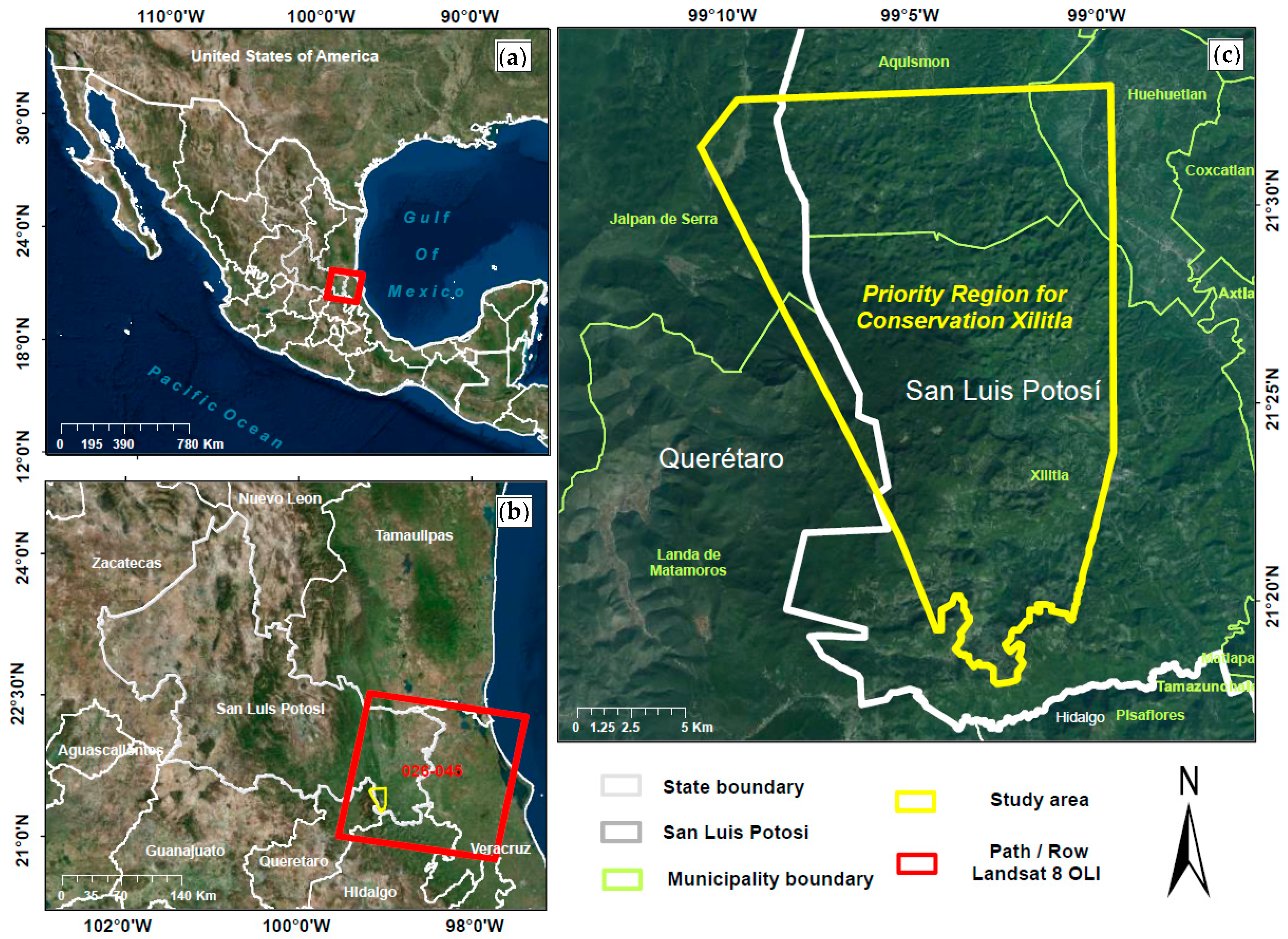
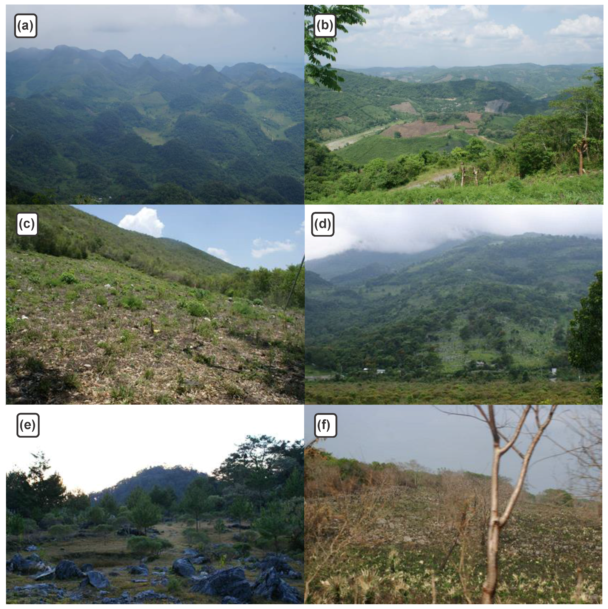
2.1. Study Area

The Priority Region for Conservation Xilitla (RPCX) is situated to the southeast of the state of San Luis Potosí (municipalities of Xilitla, Huehuetlán and Aquismón), and in the northeast of the state of Querétaro (including the municipalities Landa de Matamoros and Jalpa de Serra) in northern Mexico. The geographical location is in UTM zone 14 (21°17′46″–21°33′11″ N; 99°10′40″–98°59′12″ W, mostly contained in the municipality of Xilitla (Figure 1). The study area is located in the mountains of the Sierra Madre Oriental. Elevations range from 2950 m.a.s.l. in the highlands to 50 m.a.s.l. in the coastal plain. Wind moisture coming from the Gulf of Mexico generates an average annual precipitation of 3038 mm, and a minimum precipitation of 58 mm in the driest month of the dry season (from November to April) and a maximum precipitation of 671 mm in the rainiest month (from May to October). While, average annual temperature is 22 °C, with a minimum average of 17 °C in the warmest month and an average maximum of 26 °C in the coldest month. There are two climate types based on Köppen’s classification: Cfa [Humid subtropical with rain during all year] and Cwa [Humid subtropical with dry winter]. The soil types present in the study area are as follows: Leptosols (85.9%), Luvisols (12.2%), Feozems (1.1%) and Vertisols (0.6%). Texture varies from clay and silty soil. Vegetation type varies from cloud forest, pine forest, oak forest and pasture; however cloud forest is increasingly scarce and is located in steepest hills and poorer soils such as regosols and leptosols [32]. However, invasive plants are common in all vegetation types within the study area because of the high presence of ecological disturbances e.g., land use change mainly caused by forest fires and shifting agriculture (Figure 2).

2.2. Methodology

This research was carried out in three phases. Firstly, we used the Universal Soil Loss Equation to estimate soil erosion rate as a proxy of an urgency measure for restoration. Secondly, the Multi-Criteria Decision Analysis was applied for identifying those bare soil locations and determining its feasibility to be restored considering proximity factors. And therefore, we combined both USLE and MCDA outcomes by using a cross-tabulation matrix to identify priority land for being restored.

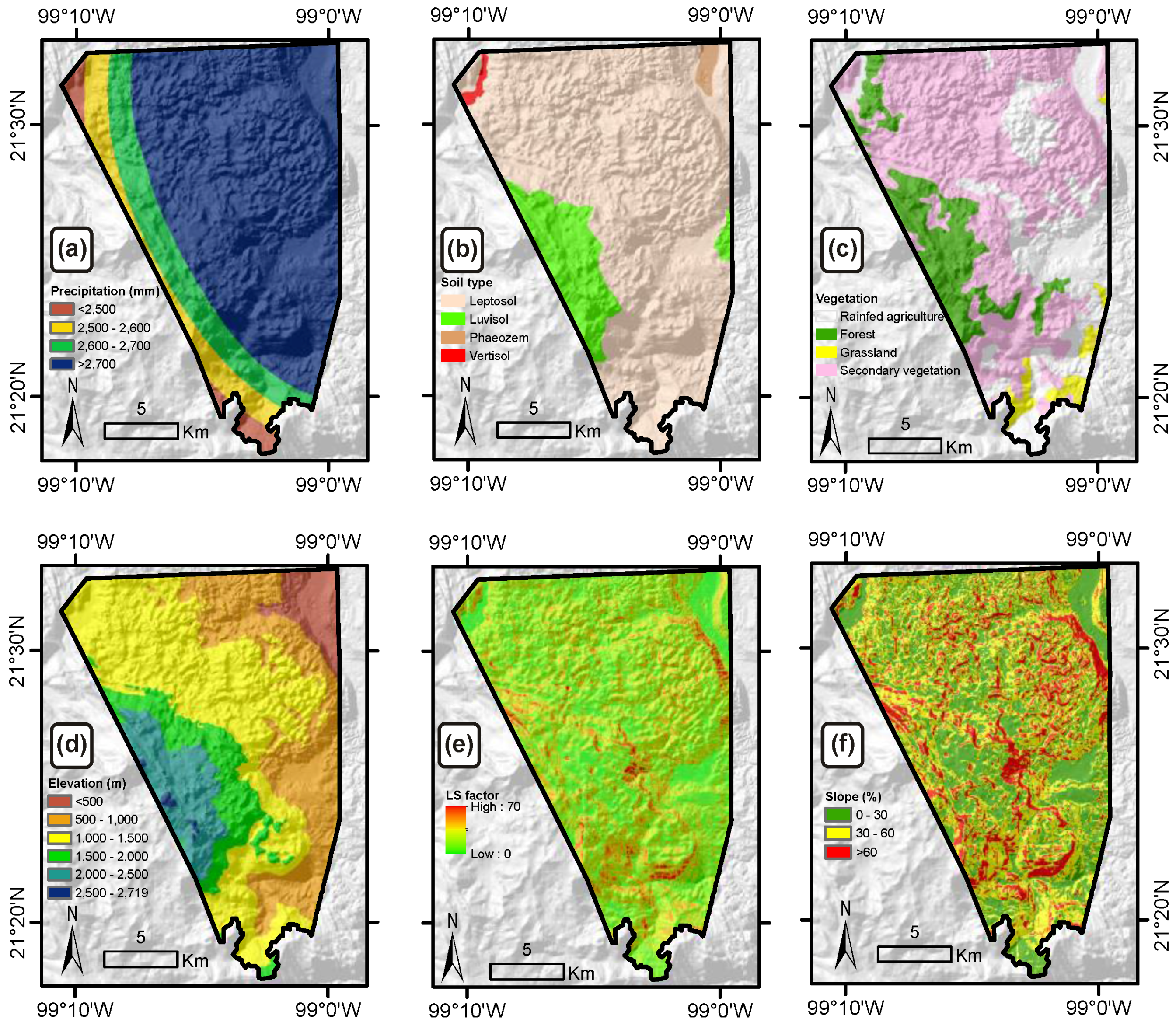
2.2.1. Universal Soil Loss Equation as a Proxy for Soil Degradation Assessment

Soil erosion was estimated by using the following equation [33,34]:

$$SLR=R\times K\times LS\times C\times P$$

(1)

where SLR is the average soil loss rate (ton·ha⁻¹·yr⁻¹), R is the factor for precipitation erosivity (MJ·mm·h⁻¹·ha⁻¹·yr⁻¹), K is the factor for soil erodibility (t·h·MJ⁻¹·mm⁻¹), LS is the combined factor for slope length and steepness (dimensionless), C is the factor for land use and land cover (dimensionless), P is the factor for management practices focused on soil conservation (dimensionless). The original variables used for determining factors used in the USLE are shown in Figure 3.

Factor R. Rainfall erosivity expresses the potential energy of raindrops to release particles from the soil and cause erosion. This index was used for a rainfall event with a maximum intensity of 30 min (EI30). For Mexico, an isoerosivity map was done at country level by analyzing 53 meteorological stations to establish 14 regions of isoerosivity [35]. The RPCX is located within in the region 13, so the formula used is as follows:

$$R=10.7427P-0.0011008P^2$$

(2)

where, R is the rainfall erosivity (MJ·mm·ha⁻¹·hr ⁻¹·yr⁻¹) and, P is the mean annual precipitation (mm). In order to obtain the annual average precipitation (P), data from 51 meteorological stations located in the area of influence (last 30 years), were interpolated by using the kriging approach in the ArcGIS version 10.2 geostatistical analyst tool (Environmental Systems Research Institute, Inc., Redlands, CA, USA). We used an ordinary kriging type, with Log transformation to make variances more constant over the entire study area and force the data to be normally distributed. The interpolation was validated by using a cross-validation technique that eliminates an observation from the dataset, fits the statistical model with the other observations, calculates the precipitation value for the eliminated observation and determine the bias (observed minus estimated value) and then determines the root mean square error (RMSE). The RMSE obtained was 283.9 mm.

K factor. Erodibility refers to the physical soil property of being eroded by water i.e., precipitation and runoff. Some characteristics influence on the degree of erodibility e.g., soil structure (texture, organic matter content). In order to obtain information about soil type and texture, we used soil data at 1:250,000 scale generated during 2002–2006 by INEGI [36]. Due to the study area was in a forested landscape, further-detail soil maps were not available for the study area. For Mexico, national covering for soil map at 1:50,000 scale is only available for agricultural valleys in the country. The soil classification used was the World Reference Base for Soil Resources. The values of erodibility used in this work were obtained by FAO [37] (

Table 1. Erodibility values according to soil type and texture in the study area.

Soil Type	Soil Texture
	Sand	Silt	Clay
Leptosol	0.053	0.079	0.026
Luvisol	0.053	0.079	0.026
Phaeozem	0.026	0.040	0.013
Vertisol	0.053	0.079	0.026

).

LS factor. The steepness and slope length are topographic factors that directly affect the soil erosion process. So, LS is a combined factor accounting the effect of slope length (L) and gradient (S). To estimate LS factor, we used the following formula developed by Moore and Burch [38,39].

$$\mathrm{LS}={\left(\frac{\mathrm{A}}{22.13}\right)}^{0.6}{\left(\frac{\sin \mathrm{B}}{0.0896}\right)}^{1.3}$$

(3)

where A is the low accumulation multiplied by cell size (m, 30 m for this case), B is the slope angle in radians. Both, flow accumulation and slope in radians were calculated using a digital elevation model obtained for the study area at 30 m pixel size from INEGI [40].

C factor. This measures the percentage of soil that can be lost when protected by a land cover type. The less vegetation cover exists, the bigger value for C factor, and then the greater soil loss. Vegetation cover represents a variable for decreasing or controlling erosion, by intercepting precipitation, increasing infiltration and reducing rainfall energy to erode soil. Figueroa et al. [41] calculated different C factor values for each coverage type. The values used for C factor are as follows: forest/secondary vegetation = 0.0001, grassland = 0.035, rainfed agriculture = 0.039 and bare soil = 0.043. Such a C factor values were assigned to a land use/land cover map obtained by applying a support vector machine algorithm. Training fields for performing the supervised classification were obtained by inspecting the Landsat scene and the vegetation and land use map Series V [42].

P factor. It refers to the impact of protecting soil from erosion by means of management practices, since they reduce runoff and consequently, the amount of soil that can be removed. It is defined as the relationship between, the amount of soil loss when protected by a conservation practice e.g., contour farming and/or terracing, to the amount of soil loss on a land cultivated in the direction of slope [43]. Commonly, this factor is obtained by digitizing conservation management practices identified in high resolution aerial imagery. But, in this case, there was no possible to detect visually in high spatial resolution imagery any soil conservation management practices; so, we used the most critical value (highest possible: 1), indicating that there was no conservation practices in the study area [44]. Once each factor was obtained, soil loss rate was calculated and classified into five classes: very low from 0 to 50 ton·ha⁻¹·yr⁻¹, low from 50 to 100 ton·ha⁻¹·yr⁻¹, middle from 100 to 150 ton·ha⁻¹·yr⁻¹, high from 150 to 200 ton·ha⁻¹·yr⁻¹, and very high higher than 200 ton·ha⁻¹·yr⁻¹.

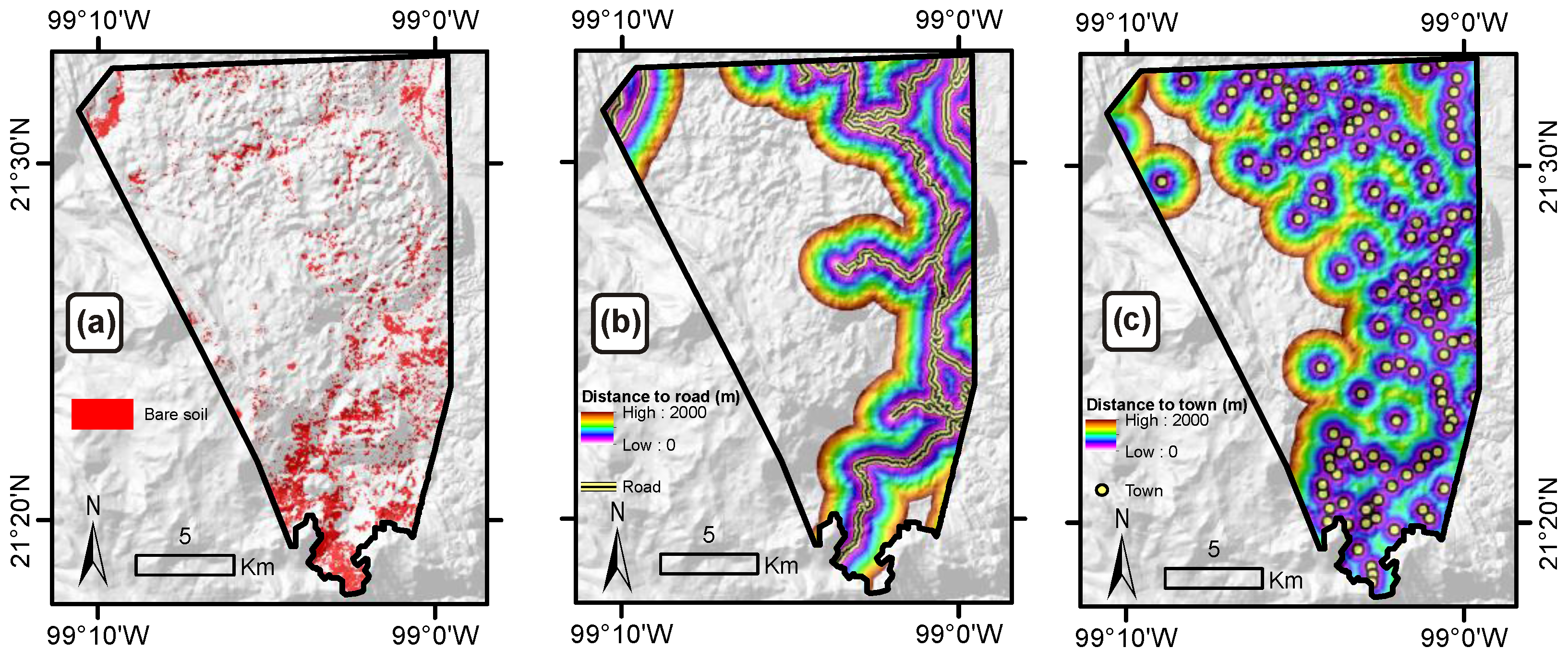
2.2.2. Multi-Criteria Decision Analysis for Determining Feasible Area to Restore

1. Factors used: distance to town/road

This approach was used to prioritize the land to be restored considering two factors and a constraint. First factor considered was population, because it is important when designing projects for ecological restoration [45]. So, 337 neighboring towns from the Priority Region for Conservation Xilitla were selected based on data from the National Institute of Statistics and Geography [46]. Hence, a map of the Euclidean distance to town at a 30 m spatial resolution was generated. Second factor was the accessibility to the priority areas to ensure the viability of the restoration project. So, the National Road Network (RNC) data was used to make the map for the factor distance to road [47,48]. Both factors (distance to town/road) were used. i.e., if the place is near to a town/road, then it is most suitable; if far, then least suitable.

Fuzzyfication process is required to standardize variables with different units of measurement and scale; it can be done by changing a real scalar value into a fuzzy value (0–1) by using a membership function. In this case, factors used are the variables distance to road/town, measured in meters. So that they are comparable and combinable, they have to be standardized by using a membership function. In this sense, such two distance factors were standardized by using a monotonically decreasing membership function denoted by the following expressions:

$$\mathrm{if}D\le 1000m\mathrm{then}{X}_i=1$$

(4)

$$\mathrm{if}D\ge 2000m\mathrm{then}{X}_i=0$$

(5)

$$\mathrm{if}1000\le D\le 2000m\mathrm{then}{X}_i=(2000-D)/1000$$

(6)

where, D is the distance to town/road, X_i is the standardized factor i with the membership functions.

In other words, the highest land suitability value = 1 was for the distance from 0 m to 1000 m and gradually decreased to 0 for those places located at/or beyond 2000 m.

In order to combine the distance to town/road map against the bare soil map, we used the weighted linear combination approach [25,49,50]. The importance values for factors were assigned equally and assumed to be 0.5. The used formula is as follows:

$$F={\displaystyle \sum _{i=1}^n{w}_i{x}_i·\underset{j=1}{\overset{k}{\Pi }}{c}_j}$$

(7)

where, F is the land feasibility to be restored, w_i is the weight for factor i and it is equal to 0.5, x_i is the standardized factor i with the membership functions; $\underset{j=1}{\overset{k}{\Pi }}{c}_j$ is the product obtained by the j constraints. i.e., bare soil obtained from a supervised classification of Landsat 8 OLI imagery spectral data.

Once land feasibility was obtained, it was classified into five classes: very low from 0 to 0.2, low from 0.2 to 0.4, middle from 0.4 to 0.6, high from 0.6 to 0.8, and very high—higher than 0.8.

2. Constraint used: bare soil map

In order to create the bare soil map for the study area, a satellite image taken by the Landsat 8 Operational Land Imager sensor during 2 January 2016 was downloaded from the Glovis Next Platform USGS and USDI [51]. The spectral bands used were as follows: Band 2—Blue (0.450–0.515 µm), Band 3—Green (0.525–0.600 µm), Band 4—Red (0.630–0.680 µm), Band 5—Near InfraRed (0.845–0.885 µm), Band 6—Short Wave InfraRed1 (1.560–1.660 µm), and Band 7—Short Wave InfraRed2 (2.100–2.300 µm). Such spectral bands were radiometrically corrected by using the following formula [52,53]:

$$P_{\lambda }=\frac{\left(Mp*Qcal+Ap\right)}{\sin \left(\theta se\right)}$$

(8)

where, P_λ is the Top-Of-Atmosphere (TOA) reflectance with correction for solar angle (dimensionless); Mp = Band-specific multiplicative rescaling factor from the metadata, called as REFLECTANCE_MULT_BAND_x, where x is the band number; Qcal = Quantized and calibrated standard product pixel values (DN); Ap = Band-specific additive rescaling factor from the metadata, called as REFLECTANCE_ADD_BAND_x, where x is the band number); sin(θse) = Local sun elevation angle. The scene center sun elevation angle in degrees is provided in the metadata found as SUN_ELEVATION.

After applying the radiometric correction to spectral data, we carried out a supervised classification by using the Vector Support Machine (SVM) algorithm. This approach employs a decision value for each landuse/landcover class to classify the pixel; in other words, a cut-off criterion is assigned (minimum probability value) as the basis for the inclusion or not of the pixel within the land use/land cover class. So, the classes are spectrally separated by a decision surface (optimal hyperplane) that maximizes the margins between classes. The nearest data (support vectors) to the optimal hyperplane are defined from training fields, which are critical elements for classification [54]. For this work, training fields were carried out for five classes: water, woodland, pasture, agriculture and bare soil, which were obtained by using a vegetation and land use map Series V [42]. The supervised classification was validated by carrying out a contingency matrix built with 100 sampling sites obtained from surveying in high spatial resolution images Google Earth platform (Google Inc., Mountain View, CA, USA). Both, the overall precision and Kappa values were 0.90 and 0.86, respectively. In consequence, the bare soil data was extracted from the created land use/land cover map, obtained from the output of the support vector machine supervised classification of Landsat 8 OLI spectral data and, it was used as a constraint in the MCDA approach (Figure 4).

2.2.3. Cross-Tabulation for Determining Priority Land to Restore

In order to select priority sites for restoration, some authors have proposed to select the top 5%, 10%, 20%, and 30% of priority areas for restoration according to several criteria [18]. However, others have compared two involved factors (i.e., environmental services and environmental risks) and selected places that maximized the value in both of them [8]. In this work, once obtained both, degraded and feasible land to restore, three levels of priority (low, middle and high priority) were determined by simply overlaying them and following the next rules (

Table 2. Decision strategy for defining priority land to restore.

			Soil Degradation Assessment by Using USLE
			Very Low	Low	Middle	High	Very High
			1	2	3	4	5
Feasibility using MCDA	Very low	1	-	-	-	-	-
	Low	2	-	-	-	-	-
	Middle	3	-	-	Low priority	Low priority	Low priority
	High	4	-	-	Middle priority	Middle priority	High priority
	Very high	5	-	-	Middle priority	High priority	High priority

). To design the decision strategy in order to select the priority sites for restoration, we divided the cross-tabulation matrix into four quadrants; the fourth quadrant was considered from middle to very high classes in both factors (soil erosion and feasibility) and was divided symmetrically in order to distribute equally the three levels of priority. The rationale of this approach was to identify the highest valued areas considering both two factors. In this case, we considered that selecting fourth quadrant would fulfill this requirement. In Figure 5 is briefly described the methodology applied in this work.

3. Results

The study area is covering 34,022.8 ha and, 13.4% of that area (4226.7 ha) is uncovered by natural vegetation (bare soil). Furthermore, 92.0% of bare soil within the study area (3890.5 ha) has climatic, edaphic, topographic conditions that lead middle, high and very high levels of soil erosion rate; while, 95.3% of the bare soil land (4030.7 ha) falls within the area with high and very high feasibility to restore. Thus, when combining USLE and MCDA outcomes, it can be revealed that 88.2% (3728.3 ha) of land is, both urgent (USLE) as well as feasible (MCDA), so it becomes a priority for restoration.

Table 3. Summary for soil erosion rate and feasibility levels in the Priority Region for Conservation Xilitla.

Level	Soil Erosion Rate USLE (ha)	Feasibility MCDA (ha)
Very low	27.0	70.4
Low	309.3	125.7
Middle	939.3	957.0
High	1955.4	961.2
Very high	995.7	2112.4
Total	4226.7	4226.7

shows both, the land classified by soil erosion rate by feasibility to restore.

Figure 6 presented the maps obtained for, (a) soil erosion calculated with the Universal Soil Loss Equation (USLE), (b) the spatial distribution of feasible sites to be restored obtained with Multicriteria Decision Analysis (MCDA), and (c) the priority areas to restore by combining two both approaches. Such maps only include bare soil pixels for being potentially ecologically restored.

Table 4. Combination of soil erosion rate and feasibility levels in the Priority Region for Conservation Xilitla for assigning priority to restore: (a) Pairwise combinations, (b) Priority areas summary, and (c) code description used for USLE/MCDA.

	(a)				(b)
USLE	MCDA	Priority	Area (ha)		Priority	Area (ha)
1	1	-	3.6		Low	858.15
1	2	-	3.8		Middle	869.67
1	3	-	3.1		High	2000.52
1	4	-	17.0		Total	4019.04
2	1	-	19.5
2	2	-	7.5
2	3	-	95.7		(c)
2	4	-	186.4		Code for USLE/MCDA	Description
3	1	-	47.8		1	Very low
3	2	-	12.1		2	Low
3	3	Low priority	304.3		3	Middle
3	4	Middle priority	154.6		4	High
3	5	Middle priority	420.3		5	Very high
4	2	-	94.41
4	3	Low priority	542.0
4	4	Middle priority	294.7
4	5	High priority	1024.2
5	2	-	7.74
5	3	Low priority	11.7
5	4	High priority	308.3
5	5	High priority	667.9
Total			4226.7

presented the detail of areas resulted from the cross-tabulation matrix. Table 4a is all possible combinations of classes for two factors and their area involved. Note that they are only for the nine pairwise comparisons that fulfilled the criteria of the fourth quadrat of the cross-tabulation matrix and Table 4b is the summarize of them. Thus, 2000.5 ha (49.7%) of land were identified with a high priority, 869.67 ha (21.6%) of land was determined as middle priority and finally 858.1 ha (21.3%) of land was as low priority. And Table 4c is the code for USLE/MCDA description used in Table 4a,b. When observing Figure 6, it is highly appreciated that soil degradation is concentrated in the center-south portion of the study area, and soil degradation increases while closer to the core city of Xilitla. A maximum degradation can be observed in the locality of Ahuacatlán de Jesús, within the municipality of Xilitla (99°03′10″ W, 21°19′13″ N), where the detail achieved with this study for detecting priority areas for making forest restoration management practices, at 30 m spatial resolution, can be appreciated. At the north portion of the study area (Municipality of Aquismon), a diminishing presence of bare soil spots was detected.

4. Discussion

This work proposed a new methodology to find the suitable sites for ecological restoration in the Priority Region for Conservation Xilitla Mexico. Such an approach combined the Universal Loss Soil Equation and Multi-Criteria Decision Analysis to find out, at pixel level, the urgent and feasible sites for ecological restoration. The evaluation method employed in this work for evaluating the feasibility of ecological restoration was the Weighted Linear Combination. The USLE model [21,55,56] and MCDA approach [49,57,58,59,60,61,62] has been normally used separately for a variety of applications. In this work, they were used as complementary. The innovative contribution of this work is the integration of two approaches by using a cross tabulation matrix for assigning the priority for restoration considering the two factors, soil erosion rate (USLE model) and feasibility (MCDA) to restore.

Environmental changes are related to a variety of social, economic and political conditions [63]; therefore, spatial models that incorporate social and economic factors interacting with biophysical processes over space and time, represent an alternative with a broad field of conceptual and methodological development [64]. High spatial resolution remotely-sensed data, i.e., Landsat 8 OLI at 30 m spatial resolution, is a useful source of spectral information to obtain the bare soil as a basis for degraded soil assessment. Several authors have also used Landsat satellite imagery, in many ways, within the methodology for estimating soil erosion. For example, Parveen and Kumar [43] used Landsat TM data to estimate C-factor by using the following equation: $\mathrm{C}={\mathrm{e}}^{\left(-\mathsf{\alpha }\left(\raisebox{1ex}{$\mathrm{NDVI}$}\!\left/ \!\raisebox{-1ex}{$\mathsf{\beta }-\mathrm{NDVI}$}\right.\right)\right)}$, where C is the C-Factor, a and b are dimensionless parameters determining the shape of the curve that relates the so-called Normalized Difference Vegetation Index (NDVI) and C-factor. Wang et al. [65] used Landsat TM and HJ satellite data to obtain land use and land cover fraction using object oriented classification for assessing soil erosion risk within a Multi-Criteria Decision Analysis framework. Borelli et al. [13] used Landsat TM and ETM sensors as ancillary data source for detecting clear-cutting at pixel level, via image differencing. Such information was used to measure the impact of clear-cutting on soil erosion in Italy. All of them represent different rationale/approaches of use of remotely sensed data when assessing soil erosion risk. In this work, we used Landsat spectral data for determining bare soil by applying the support vector machine algorithm [54] in order to find those most urgent sites that require to be ecologically restored. It is important to mention that, the quality of results obtained is often limited by the level of detail of the available data sources i.e., spatial and temporal. In our case, there was only availability of Landsat spectral data at 30 m spatial resolution [66], so the level of detail achieved can be improved; thus, further research can be addressed to use higher spatial resolution sensors i.e., Geoeye, Worldview or Quickbird, in order to find, more accurately, the bare soil land that urgently requires being ecologically restored. However, the large size of study area and the cloudy environment make difficult to build a seamless dataset with high spatial resolution imagery that cover all the study area.

Distance to roads [48,67] and distance to town [68,69] were considered to be sufficient number of variables required to the MCDA modeling, because the interest of this research was, on where are the nearest sites to restore that are more urgent. Such a sites are planning to be restored by revegetation with local species to assure regeneration of the forest site. So, the best places to accomplish this objective were those that are most eroded and near to towns and roads. The interest of restoring in this natural protected area is to prevent from erosion. There are not water bodies in the study area; the value of land, in terms of real state, can be neglected because it is a sparsely populated, rural area. Probably, the environmental service of habitat for wildlife could be considered, but, in this case, the only motivation was how to protect more efficiently soil from erosion by revegetation in this Priority Region for Conservation Xilitla.

Several approaches have been developed for delineating priority sites for restoration. Some authors have carried out studies on land use change (i.e., deforestation) by using two date maps created by remotely-sensed data, in order to detect deforested land, and making it candidate for restoration [6,70,71]. Others have identified priority areas for restoration according to environmental quality. For example, Rahman et al. [30] identified by designing an environmental quality index encompassing a set of factors such as landscape ecology, natural hazards, climate, topography, soil environment and demography by coupling remotely sensed and geospatial information in a multi-criteria decision analysis; the lower environmental quality index, the higher priority for environmental restoration.

This study area has been affected by climate change because it has been experienced drought during the last twenty years [72,73]. Furthermore, high rates of change to which ecosystems are subjected suggest urgent attention to deforestation and degradation [74]. Deforestation processes in the RPCX could lead to increase erosion and landslide events, mainly due to forest cover conversion [75,76]. Moreover, intense rainfall events presented in the barlovento region of the Huasteca Potosina, trigger soil erosion on bare land. Subsequently, soil loss rate is a serious problem for maintaining an ecosystem healthy, because soil supports all living organisms into the ecosystem and once lost, it is very difficult to recover. Thus, forest restoration activities must be carefully planned in order to identify the best places for growing tree species for soil recovery.

The Mexican government through several institutions has been always shown a strong interest in conserving/restoring and managing ecosystems while promoting sustainable development [31]. In order to achieve sustainability goals, it is mandatory to implement adequate approaches for both assessing land degradation and proposing suitable alternatives for ecosystem restoration. Hence, the relevance of the application of this methodology is, for optimizing the use of economic funds for ecological restoration activities.

In Mexico, there are a total of 177 natural protected areas by the federal government [77] and only a half of them has management program for protecting natural resources. In several management programs are indicated the requirement of spatially evaluating soil erosion in order to locate specifically the areas for ecological restoration. However, there is a lack of detailed maps depicting soil erosion in such management programs of natural protected areas (please visit http://www.conanp.gob.mx/movil/programas.php). So, there is a current need for making studies that can be used as a tool for stakeholders and decision makers for planning ecosystem restoration practices.

The proposed methodology constitutes a reliable tool for selecting sites for revegetation in Mexico, becoming relevant given the great richness of biodiversity of the country [78]. Particularly, for natural protected areas, this study means a contribution to the knowledge of science due to the lack of scientific reports of its kind, and especially to the threats faced by future ecological processes [79]. That is, the concern of revegetating degraded areas, is consistent with the processes of ecological succession [80]. Consequently, the proper identification of urgent areas to be restored is the first step. In addition, the anthropogenic causes in their role of explanatory variables [6], give scientific support to the results (Figure 6, Table 3). These indicators represent crucial elements of decision-making for local managers [81], so additional research efforts to balance the effectiveness of landscape management [82] with socio-economic interests [83] are not ruled out. Ecological restoration is a manipulative activity and explicitly experimental [71], so we would like to specify that our approach can be used as an alternative, to spatially locate the sites that require an urgent work for ecosystem restoration and besides are feasible to restore.

5. Conclusions

The combination of the Universal Soil Loss Equation (USLE) and Multicriteria Decision Analysis (MCDA) to prioritize the sites to be ecologically-restored was applied in the Priority Region for Conservation Xilitla, in the state of San Luis Potosí (Mexico). Thus, an integral approach was used to locate sites for restoration as well as their prioritization considering the feasibility determined by the distance to town and road. In this research work, after processing Landsat 8 OLI spectral data, we found out that 13% (4226.94 ha) of the total area of the Priority Region for Conservation Xilitla is covered by bare soil. The methodology applied in this research also figured out that higher than 90% of bare soil is in middle, high and very high levels of soil erosion rate; and 88.20% of bare soil land (3728.34 ha) is priority to restore. Soil erosion is not uniformly distributed within in the study area; it can be commonly visualized in the eastern part of the Priority Region for Conservation Xilitla, with a north-south pattern and following the main road, becoming a serious problem near to Xilitla. This methodology is transparent and replicable, so it could be used by stakeholders, in other latitudes with local adaptations, in order to wisely destine economic funds for planning and making forest ecosystem restoration practices in natural protected areas around the world.

References

1. Lal, R. Restoring soil quality to mitigate soil degradation. Sustainability 2015, 7, 5875–5895. [Google Scholar] [CrossRef]
2. Muñoz-Iniestra, D.J.; Ferreira-Ramírez, M.; Berenice, E.A.I.; López-García, J. Relación entre la cobertura de suelo y la degradación física y biológica de un suelo aluvial en una región semiárida. Terra Latinoamericana 2013, 31, 201–210. [Google Scholar]
3. Ramírez-Carballo, H.; Pedroza-Sandoval, A. Participatory assessment of the soil degradation in Biosphere Reserve Mapimí, Durango, México. Revista Chapingo Serie Zonas Áridas 2007, 6, 247–254. [Google Scholar]
4. Vargas Ríos, O. Restauración ecológica: Biodiversidad y conservación. Acta Biológica Colombiana 2011, 16, 221–246. [Google Scholar]
5. Yin, R.; Zhao, M. Ecological restoration programs and payments for ecosystem services as integrated biophysical and socioeconomic processes—China’s experience as an example. Ecol. Econ. 2012, 73, 56–65. [Google Scholar] [CrossRef]
6. Reddy, C.S.; Manaswini, G.; Satish, K.V.; Singh, S.; Jha, C.S.; Dadhwal, V.K. Conservation priorities of forest ecosystems: Evaluation of deforestation and degradation hotspots using geospatial techniques. Ecol. Eng. 2016, 91, 333–342. [Google Scholar] [CrossRef]
7. Adame, M.F.; Hermoso, V.; Perhans, K.; Lovelock, C.E.; Herrera-Silveira, J.A. Selecting cost-effective areas for restoration of ecosystem services. Conserv. Biol. 2015, 29, 493–502. [Google Scholar] [CrossRef] [PubMed]
8. Trabucchi, M.; O’Farrell, P.J.; Notivol, E.; Comín, F.A. Mapping ecological processes and ecosystem services for prioritizing restoration efforts in a semi-arid mediterranean river basin. Environ. Manag. 2014, 53, 1132–1145. [Google Scholar] [CrossRef] [PubMed]
9. Trabucchi, M.; Comín, F.A.; O’Farrell, P.J. Hierarchical priority setting for restoration in a watershed in NE Spain, based on assessments of soil erosion and ecosystem services. Reg. Environ. Chang. 2013, 13, 911–926. [Google Scholar] [CrossRef] [Green Version]
10. Jacobs, D.F.; Oliet, J.A.; Aronson, J.; Bolte, A.; Bullock, J.M.; Donoso, P.J.; Landhäusser, S.M.; Madsen, P.; Peng, S.; Rey-Benayas, J.M.; et al. Restoring forests: What constitutes success in the twenty-first century? New For. 2015, 46, 601–614. [Google Scholar] [CrossRef]
11. Shriver, D.M.; Randhir, T.O. Integrating Stakeholder Values with Multiple Attributes to Quantify Watershed Performance. Water Resour. Res. 2006, 42. [Google Scholar] [CrossRef]
12. Bana e Costa, C.A.; Antao da Silva, P.; Nunes Correia, F. Multicriteria Evaluation for Flood Control Measures: The Case of Ribeira Do Livramento; The London School of Economics and Political Science: London, UK, 2003. [Google Scholar]
13. Borrelli, P.; Panagos, P.; Märker, M.; Modugno, S.; Schütt, B. Assessment of the impacts of clear-cutting on soil loss by water erosion in Italian forests: First comprehensive monitoring and modelling approach. Catena 2017, 149, 770–781. [Google Scholar] [CrossRef]
14. Meshesha, D.T.; Tsunekawa, A.; Tsubo, M.; Haregeweyn, N. Dynamics and hotspots of soil erosion and management scenarios of the central rift valley of Ethiopia. Int. J. Sediment Res. 2012, 27, 84–99. [Google Scholar] [CrossRef]
15. Duarte, G.T.; Ribeiro, M.C.; Paglia, A.P. Ecosystem services modeling as a tool for defining priority areas for conservation. PLoS ONE 2016, 11, e0154573. [Google Scholar] [CrossRef]
16. Thomson, J.R.; Moilanen, A.J.; Vesk, P.A.; Bennett, A.F.; Mac Nally, R. Where and when to revegetate: A quantitative method for scheduling landscape reconstruction. Ecol. Appl. 2009, 19, 817–828. [Google Scholar] [CrossRef] [PubMed]
17. Moilanen, A.; Leathwick, J.R.; Quinn, J.M. Spatial prioritization of conservation management. Conserv. Lett. 2011, 4, 383–393. [Google Scholar] [CrossRef]
18. Legge, J.T.; Doran, P.J.; Herbert, M.E.; Asher, J.; O’Neil, G.; Mysorekar, S.; Sowa, S.; Hall, K.R. From model outputs to conservation action: Prioritizing locations for implementing agricultural best management practices in a midwestern watershed. J. Soil Water Conserv. 2013, 68, 22–33. [Google Scholar] [CrossRef]
19. Richardson, M.S.; Gatti, R.C. Prioritizing wetland restoration activity within a Wisconsin watershed using GIS modeling. J. Soil Water Conserv. 1999, 54, 537–542. [Google Scholar]
20. Widis, D.C.; BenDor, T.K.; Deegan, M. Prioritizing wetland restoration sites: A review and application to a large-scale coastal restoration program. Ecol. Restor. 2015, 33, 358–377. [Google Scholar] [CrossRef]
21. Mohamed, E.S.; Schütt, B.; Belal, A. Assessment of environmental hazards in the North Western Coast Egypt using RS and GIS. Egypt. J. Remote Sens. Space Sci. 2013, 16, 219–229. [Google Scholar] [CrossRef]
22. Teshome, A.; Rolker, D.; de Graaff, J. Financial viability of soil and water conservation technologies in northwestern Ethiopian highlands. Appl. Geogr. 2013, 37, 139–149. [Google Scholar] [CrossRef]
23. Mancino, G.; Nolè, A.; Salvati, L.; Ferrara, A. In-between forest expansion and cropland decline: A revised USLE model for soil erosion risk under land-use change in a Mditerranean region. Ecol. Indic. 2016, 71, 544–550. [Google Scholar] [CrossRef]
24. Alexandridis, T.K.; Sotiropoulou, A.M.; Bilas, G.; Karapetsas, N.; Silleos, N.G. The effects of seasonality in estimating the C-factor of soil erosion studies. Land Degrad. Dev. 2015, 26, 596–603. [Google Scholar] [CrossRef]
25. Malczewski, J. GIS-based land-use suitability analysis: A critical overview. Prog. Plan. 2004, 62, 3–65. [Google Scholar] [CrossRef]
26. Stemn, E.; Kumi-Boateng, B.; Sibil, S. Multi-criteria-GIS based site selection for irrigational reservoir—A case study. Eur. Agrophys. J. 2016, 3, 1–17. [Google Scholar] [CrossRef]
27. Uribe, D.; Geneletti, D.; del Castillo, R.; Orsi, F. Integrating stakeholder preferences and GIS-based multicriteria analysis to identify forest landscape restoration priorities. Sustainability 2014, 6, 935–951. [Google Scholar] [CrossRef]
28. Orsi, F.; Geneletti, D. Identifying priority areas for forest landscape restoration in Chiapas (Mexico): An operational approach combining ecological and socioeconomic criteria. Landsc. Urban Plan. 2010, 94, 20–30. [Google Scholar] [CrossRef]
29. Patel, D.P.; Srivastava, P.K.; Gupta, M.; Nandhakumar, N. Decision support system integrated with geographic information system to target restoration actions in watersheds of arid environment: A case study of Hathmati watershed, Sabarkantha district, Gujarat. J. Earth Syst. Sci. 2015, 124, 71–86. [Google Scholar] [CrossRef]
30. Rahman, M.R.; Shi, Z.H.; Chongfa, C. Assessing regional environmental quality by integrated use of remote sensing, GIS, and spatial multi-criteria evaluation for prioritization of environmental restoration. Environ. Monit. Assess. 2014, 186, 6993–7009. [Google Scholar] [CrossRef] [PubMed]
31. CONANP; GIZ. Programa de Adaptación al Cambio Climático de la Región Central de la Sierra Madre Oriental; Comisión Nacional de Áreas Naturales Protegidas, Deutsche Gesellschaft für Internationale Zusammenarbeit: Mexico City, Mexico, 2013. [Google Scholar]
32. Reyes-Hernández, H.; Aguilar-Robledo, M.; Aguirre-Rivero, J.; Trejo-Vázquez, I. Cambios en la cubierta vegetal y uso del suelo en el área del proyecto Pujal-Coy, San Luis Potosí, México. Investigaciones Geográficas 2006, 59, 26–42. [Google Scholar]
33. Renard, K.G.; Foster, G.R.; Weesies, G.A.; McCool, D.K.; Yoder, D.C. Predicting Soil Erosion by Water: A Guide to Conservation Planning with the Revised Universal Soil Loss Equation; U.S. Department of Agriculture, Agricultural Research Service: Beltsville, MD, USA, 1997; p. 384.
34. Wischmeier, W.H.; Smith, D.D. Predicting Rainfall Erosion Losses. A Guide to Conservation Planning; U.S. Department of Agriculture: Beltsville, MD, USA, 1978.
35. Cortés, T.H. Caracterización de la Erosividad de la Lluvia en México Utilizando Métodos Multivariados. Master’s Thesis, Colegio de Postgraduados, Montecillo, Mexico, 1991. [Google Scholar]
36. INEGI. Conjunto de Datos Vectoriales Edafológico Escala 1:250,000; Serie II; National Institute of Statistics and Geography (Mexico): Aguascalientes, Mexico, 2006. [Google Scholar]
37. Food and Agriculture Organization (FAO). A Provisional Methodology for Soil Degradation Assessment; FAO: Rome, Italy, 1979. [Google Scholar]
38. Moore, I.D.; Burch, G.J. Physical basis of the length slope factor in the Universal Soil Loss Equation. Soil Sci. Soc. Am. J. 1986, 50, 1294–1298. [Google Scholar] [CrossRef]
39. Moore, I.D.; Burch, G.J. Modeling erosion and deposition: Topographic effects. Trans. Am. Soc. Agric. Eng. 1986, 29, 1624–1630. [Google Scholar] [CrossRef]
40. INEGI. Digital Elevation Model at 30 m Spatial Resolution; National Institute of Statistics and Geography: Aguascalientes, Mexico, 2013. [Google Scholar]
41. Figueroa, S.B.; Amante, A.O.; Cortes, H.G.T.; Pimentel, J.; Osuna, C.E.S.; Rodríguez, O.; Morales, F.J. Manual de Predicción de Perdidas de Suelo Por Erosión; Secretaria de Agricultura y Recursos Hidráulicos Colegio de Postgraduados: Montecillo, Mexico, 1991; p. 150. [Google Scholar]
42. INEGI. Conjunto de Datos Vectoriales de Uso de Suelo y Vegetación, Escala 1:250 000; Serie V (Continuo Nacional); Instituto Nacional de Estadística y Geografia: Aguascalientes, Mexico, 2013. [Google Scholar]
43. Parveen, R.; Kumar, U. Integrated approach of Universal Soil Loss Equation and Geographical Information System for soil loss risk assessment in Upper South Koel basin, Jharkhand. J. Geogr. Inf. Syst. 2012, 4, 588–596. [Google Scholar] [CrossRef]
44. Correa, S.W.; Mello, C.R.; Chou, S.C.; Curi, N.; Norton, L.D. Soil erosion risk associated with climate change at Mantaro River basin, Peruvian Andes. Catena 2016, 147, 110–124. [Google Scholar] [CrossRef]
45. Wilson, S.J.; Cagalanan, D. Governing restoration: Strategies, adaptations and innovations for tomorrow’s forest landscapes. World Dev. Perspect. 2016, 4, 11–15. [Google Scholar] [CrossRef]
46. INEGI. Marco Geoestadístico Nacional, 6.2 ed.; Instituto Nacional de Estadística y Geografía: Aguascalientes, Mexico, 2014. [Google Scholar]
47. INEGI. Conjunto de Datos Vectoriales de Carreteras y Vialidades urbanas, edición 1.0; Instituto Nacional de Estadística y Geografía: Aguascalientes, Mexico, 2016. [Google Scholar]
48. Braid, A.C.; Nielsen, S.E. Prioritizing sites for protection and restoration for grizzly bears (Ursus arctos) in Southwestern Alberta, Canada. PLoS ONE 2015, 10, e0132501. [Google Scholar] [CrossRef] [PubMed]
49. Averna-Valente, R.D.O.; Vettorazzi, C.A. Definition of priority areas for forest conservation through the Ordered Weighted Averaging method. For. Ecol. Manag. 2008, 256, 1408–1417. [Google Scholar] [CrossRef]
50. Drobne, S.; Lisec, A. Multi-attribute decision analysis in GIS: Weighted Linear Combination and Ordered Weighted Averaging. Informatica 2009, 33, 459–474. [Google Scholar]
51. USGS; USDI. Global Visualization (GloVis) Viewer. Available online: https://glovis.usgs.gov/ (accessed on 22 August 2017).
52. Ariza, A. Descripción y Corrección de Productos Landsat 8; Instituto Geográfico Agustín Codazzi: Bogotá, Colombia, 2013. [Google Scholar]
53. USGS. Using the USGS Landsat 8 Product; United States Geological Survey: Reston, VA, USA, 2016.
54. Stević, D.; Hut, I.; Dojčinović, N.; Joković, J. Automated identification of land cover type using multispectral satellite images. Energy Build. 2016, 115, 131–137. [Google Scholar] [CrossRef]
55. Mahalingam, B.; Malik, M.M.; Vinay, M. Assessment of soil erosion using USLE technique: A case study of Mysore district, Karnataka, India. J. Remote Sens. GIS 2015, 6, 1–7. [Google Scholar]
56. Zhang, X.; Wu, B.; Ling, F.; Zeng, Y.; Yan, N.; Yuan, C. Identification of priority areas for controlling soil erosion. Catena 2010, 83, 76–86. [Google Scholar] [CrossRef]
57. Aydin, N.Y.; Kentel, E.; Duzgun, S. GIS-based environmental assessment of wind energy systems for spatial planning: A case study from western turkey. Renew. Sustain. Energy Rev. 2010, 14, 364–373. [Google Scholar] [CrossRef]
58. Chang, N.B.; Parvathinathan, G.; Breeden, J.B. Combining GIS with fuzzy multicriteria decision-making for landfill siting in a fast-growing urban region. J. Environ. Manag. 2008, 87, 139–153. [Google Scholar] [CrossRef] [PubMed]
59. Fernández, I.C.; Morales, N.S. A spatial multicriteria decision analysis for selecting priority sites for plant species restoration: A case study from the Chilean biodiversity hotspot. Restor. Ecol. 2016, 24, 599–608. [Google Scholar] [CrossRef]
60. Comino, E.; Bottero, M.; Pomarico, S.; Rosso, M. Exploring the environmental value of ecosystem services for a river basin through a spatial multicriteria analysis. Land Use Policy 2014, 36, 381–395. [Google Scholar] [CrossRef]
61. Bottero, M.; Comino, E.; Duriavig, M.; Ferretti, V.; Pomarico, S. The application of a Multicriteria Spatial Decision Support System (MCSDSS) for the assessment of biodiversity conservation in the province of Varese (Italy). Land Use Policy 2013, 30, 730–738. [Google Scholar] [CrossRef]
62. Ferretti, V.; Pomarico, S. Ecological land suitability analysis through spatial indicators: An application of the Analytic Network Process technique and Ordered Weighted Average approach. Ecol. Indic. 2013, 34, 507–519. [Google Scholar] [CrossRef]
63. Pijanowski, B.C.; Brown, D.G.; Shellito, B.A.; Manik, G.A. Using neural networks and GIS to forecast land use changes: A land transformation model. Comput. Environ. Urban Syst. 2002, 26, 553–575. [Google Scholar] [CrossRef]
64. Mas, J.F.; Puig, H.; Palacio, P.; Sosa, A. Modelado del proceso de deforestación en una región del sureste de México. In Proceedings of the II Seminario Latinoamericano de Geografía Física, Maracaibo, Venezuela, 24–27 July 2002. [Google Scholar]
65. Wang, L.; Huang, J.; Du, Y.; Hu, Y.; Han, P. Dynamic assessment of soil erosion risk using Landsat TM and HJ satellite data in Danjiangkou Reservoir Area, China. Remote Sens. 2013, 5, 3826–3848. [Google Scholar] [CrossRef]
66. Minaei, M.; Kainz, W. Watershed land cover/land use mapping using remote sensing and data mining in Gorganrood, Iran. ISPRS Int. J. Geoinf. 2016, 5, 57. [Google Scholar] [CrossRef]
67. Fedy, B.C.; Doherty, K.E.; Aldridge, C.L.; O’Donnell, M.; Beck, J.L.; Bedrosian, B.; Gummer, D.; Holloran, M.J.; Johnson, G.D.; Kaczor, N.W.; et al. Habitat prioritization across large landscapes, multiple seasons, and novel areas: An example using greater sage-grouse in Wyoming. Wildl. Monogr. 2014, 190, 1–39. [Google Scholar] [CrossRef]
68. Sattler, T.; Bontadina, F.; Hirzel, A.H.; Arlettaz, R. Ecological niche modelling of two cryptic bat species calls for a reassessment of their conservation status. J. Appl. Ecol. 2007, 44, 1188–1199. [Google Scholar] [CrossRef]
69. Martínez-Harms, M.J.; Quijas, S.; Merenlender, A.M.; Balvanera, P. Enhancing ecosystem services maps combining field and environmental data. Ecosyst. Serv. 2016, 22, 32–40. [Google Scholar] [CrossRef]
70. Budiharta, S.; Meijaard, E.; Wells, J.A.; Abram, N.K.; Wilson, K.A. Enhancing feasibility: Incorporating a socio-ecological systems framework into restoration planning. Environ. Sci. Policy 2016, 64, 83–92. [Google Scholar] [CrossRef]
71. Marignani, M.; Rocchini, D.; Torri, D.; Chiarucci, A.; Maccherini, S. Planning restoration in a cultural landscape in Italy using an Object-based Approach and historical analysis. Landsc. Urban Plan. 2008, 84, 28–37. [Google Scholar] [CrossRef]
72. Jabardo-Pereda, V.; Padilla-y-Sotelo, L.S. Water scarcity in the Huasteca Potosina (México): Local conflicts. Rev. Univ. Geogr. 2016, 25, 133. [Google Scholar]
73. SEMARNAT. Consecuencias Sociales del Cambio Climático en México: Análisis y Propuestas; Secretaria del Medio Ambiente y Recursos Naturales: Villahermosa, Mexico, 2009; p. 67. [Google Scholar]
74. Miranda-Aragón, L.; Treviño-Garza, E.J.; Jiménez-Pérez, J.; Aguirre-Calderón, O.A.; González-Tagle, M.A.; Pompa-García, M.; Aguirre-Salado, C.A. Modeling susceptibility to deforestation of remaining ecosystems in North Central Mexico with logistic regression. J. For. Res. 2012, 23, 345–354. [Google Scholar] [CrossRef]
75. Lambin, E.F. Modelling and monitoring land-cover change processes in tropical regions. Prog. Phys. Geogr. 1997, 21, 375–393. [Google Scholar] [CrossRef]
76. Grau, H.R.; Mitchell, T.A.; Zimmerman, J.K.; Thomlinson, J.R.; Helmer, E.; Xioming, Z. The ecological consequences of socioeconomic and land-use changes in postagriculture Puerto Rico. BioScience 2003, 53, 1159–1168. [Google Scholar] [CrossRef]
77. CONANP. Management Programs of Natural Protected Areas in Mexico. Available online: http://www.conanp.gob.mx/movil/programas.php (accessed on 13 August 2017).
78. Garcia-Alaniz, N.; Equihua, M.; Pérez-Maqueo, O.; Equihua Benítez, J.; Maeda, P.; Pardo Urrutia, F.; Flores Martínez, J.J.; Villela Gaytán, S.A.; Schmidt, M. The Mexican National Biodiversity and Ecosystem Degradation Monitoring System. Curr. Opin. Environ. Sustain. 2017, 26–27, 62–68. [Google Scholar] [CrossRef]
79. Pompa-García, M.; González-Cásares, M.; Acosta-Hernández, A.; Camarero, J.; Rodríguez-Catón, M. Drought influence over radial growth of mexican conifers inhabiting mesic and xeric sites. Forests 2017, 8, 175. [Google Scholar] [CrossRef]
80. An, S.-S.; Darboux, F.; Cheng, M. Revegetation as an efficient means of increasing soil aggregate stability on the Loess Plateau (China). Geoderma 2013, 209–210, 75–85. [Google Scholar] [CrossRef]
81. Peralta-Rivero, C.; Galindo-Mendoza, M.G.; Contreras-Servín, C.; Algara-Siller, M.; Mas-Caussel, J.F. Local perception regarding to the environmental assessment and loss of forest resources in the Huasteca Region of San Luis Potosi, Mexico. Madera y Bosques 2016, 22, 71–93. [Google Scholar]
82. Sayer, J.A.; Margules, C.; Boedhihartono, A.K.; Sunderland, T.; Langston, J.D.; Reed, J.; Riggs, R.; Buck, L.E.; Campbell, B.M.; Kusters, K.; et al. Measuring the effectiveness of landscape approaches to conservation and development. Sustain. Sci. 2016, 12, 465–476. [Google Scholar] [CrossRef]
83. Sanchez-Cuervo, A.M.; Aide, T.M. Identifying hotspots of deforestation and reforestation in Colombia (2001–2010): Implications for protected areas. Ecosphere 2013, 4, 1–21. [Google Scholar] [CrossRef]
Figure 1. Study area. (a) Location of study area; (b) Landsat 8 Operational Land Imager (OLI) sensor scene—path/row: 026/045, taken during 2 January 2016; (c) border of Priority Region for Conservation Xilitla at the municipalities involved.
Ijgi 06 00262 g001
Figure 2. Six sites in the study area. (a) Location name: La Herradura (21°25′55.75″ N, 99°02′42.83″ W), description: shifting cultivation as a land use change driver in the Priority Region for Conservation Xilitla (Mexico); (b) Location name: Las Joyas, Xilitla (21°26′03.49″ N, 99°02′49.62″ W), description: hilly terrain and land use change; (c) Location name: Near to Ollita del Pino, Xilitla (21°22′53.09″ N, 99°03′13.8″ W), description: land deforested by shifting cultivation; (d) Location name: Near to Rancho Nuevo, Xilitla (21°26′20.89″ N, 99°02′25.41″ W), description: hilly terrain and land use change; (e) Location name: La Trinidad, Xilitla (21°24′13″ N, 99°04′21″ W), description: land for pasture in hilly terrain; (f) Location name: Near to Tangojo (21°30′26.51″ N, 99°04′39.1″ W), description: land use change by shifting cultivation.
Ijgi 06 00262 g002
Figure 3. Variables used for determining the soil-loss-related factors employed in the USLE equation. (a) Mean annual precipitation for estimating the R factor; (b) Soil type for assigning a K Factor; (c) land use/land cover map to create the training fields for supervised classification and assigning the C factor; (d) digital elevation model for calculating the (e) LS factor and (f) the terrain slope.
Ijgi 06 00262 g003
Figure 4. Variables used in the MCDA approach for estimating the feasibility to restore. (a) Bare soil map obtained by supervised classification of Landsat 8 OLI spectral data; (b) Distance to road; (c) Distance to town.
Ijgi 06 00262 g004
Figure 5. Flowchart of the methodology used.
Ijgi 06 00262 g005
Figure 6. Degraded land in the Priority Region for Conservation Xilitla. (a) soil erosion rate by USLE, (b) feasible land to restore according distance to town/road by applying MCDA, (c) priority areas for restoration integrating USLE and MCDA; (df) are a zoom-in to a detailed location into the study area.
Ijgi 06 00262 g006