Public Transit Route Mapping for Large-Scale Multimodal Networks


1
TEAMverkehr.zug AG, 6330 Cham, Switzerland
2
Institut für Verkehrsplanung und Transportsysteme (IVT), ETH Zurich, 8093 Zurich, Switzerland
*
Author to whom correspondence should be addressed.
ISPRS Int. J. Geo-Inf. 2017, 6(9), 268; https://0-doi-org.brum.beds.ac.uk/10.3390/ijgi6090268
Submission received: 29 June 2017
/
Revised: 10 August 2017
/
Accepted: 21 August 2017
/
Published: 26 August 2017
(This article belongs to the Special Issue Geospatial Big Data and Transport)
Abstract
:For the simulation of public transport, next to a schedule, knowledge of the public transport routes is required. While the schedules are becoming available, the precise network routes often remain unknown and must be reconstructed. For large-scale networks, however, a manual reconstruction becomes unfeasible. This paper presents a route reconstruction algorithm, which requires only the sequence and positions of the public transport stops and the street network. It uses an abstract graph to calculate the least-cost path from a route’s first to its last stop, with the constraint that the path must contain a so-called link candidate for every stop of the route’s stop sequence. The proposed algorithm is implemented explicitly for large-scale, real life networks. The algorithm is able to handle multiple lines and modes, to combine them at the same stop location (e.g., train and bus lines coming together at a train station), to automatically reconstruct missing links in the network, and to provide intelligent and efficient feedback if apparent errors occur. GPS or OSM tracks of the lines can be used to improve results, if available. The open-source algorithm has been tested for Zurich for mapping accuracy. In summary, the new algorithm and its MATSim-based implementation is a powerful, tested tool to reconstruct public transport network routes for large-scale systems.
1. Introduction
Public transit (PT) vehicles, such as buses, interact with private traffic. They can get stuck in traffic, which leads to delays, or they can cause traffic jams if they stop at on-street public transit stops. System-wide studies on these interactions and how they can be optimized is an increasingly frequent subject of transportation studies (e.g., [1,2,3,4]). However, to observe such interaction effects in system-wide transport simulations, precise routes of the public transit vehicles are required. Additionally, correct network routes also improve the visualization and credibility of simulation results. Usually, such network routes are not available from public transit data sources and have to be generated. For instance, the schedule format HAFAS [5], which is a popular format in Central Europe, provides only the stop sequence of a transit route. The worldwide more popular and newer General Transit Feed Specification (GTFS) [6] provides optional specifications to store network routes and/or geo-referenced tracks of PT vehicles. Until now, however, most feeds do not provide this data (see Transitland [7]). In addition, depending on input data, precise stop locations are often unavailable. In many schedules, multiple stop locations on different roads are combined into one parent stop with the same name.
Transit route information provided by map-based data sources, for example Open Street Map [8] (OSM), is readily available and keeps growing. However, these sources usually lack schedule information. An additional difficulty in the special case of OSM—developing steadily into the standard database for network creation in transport modeling—is that no guarantee is given for completeness and accuracy of the data. Therefore, at least up to now, OSM could be used for multimodal networks only in combination with other data sources. Thus, today, an additional mapping step is almost always required to create a multimodal transport supply model for transport simulations.
Some literature exists on how to map routes if GPS tracks are available [9,10]. As mentioned above, however, such data is rarely available for all routes of a schedule and collecting this data for large areas is expensive. A general solution for the creation of multimodal transport supply should therefore work without GPS tracks, but incorporate them if they are available. In addition, the approaches used for mapping GPS data points to a network are rarely applicable for public transit data. Point density is vastly lower with each stop representing only one data point, whereas GPS data provides multiple points even between two stops.
Literature on mapping public transit routes to a network without using GPS data is rather sparse. Bösch and Ciari [11] provide such an algorithm; it looks for the closest node from a stop facility and then the nearest outlink. This link is set as the reference link for this stop facility. Then, the shortest path between all reference links is calculated. If there are no nodes within a given search radius, a new node is created at the stop facility’s location and this node is connected with an artificial link to the previous stop link’s end node. The artificial link is set as the stop facility’s reference link, ensuring that all stop facilities can be accessed and a valid schedule can be created.
Ordonez and Erath [12] propose a semi-automatic procedure using only one link per stop, with an automatic map-matching algorithm performed for a route. The algorithm goes through all stops and identifies the shortest path from the previous stop’s link to the current stop’s link. If a stop does not have a link referenced, a set of link candidates is created. The shortest path is calculated from the previous stop link to each defined candidate. The shortest path algorithm includes travel time and distance to the GPS points for link costs; the path with the lowest cost is part of the solution and its last link is selected and assigned to the stop. The reference link for the first stop is identified similarly. Once a link is referenced to a stop facility, all other transit routes using this stop must use this link, which makes the order of the transit routes assignment crucial. The created path is verified automatically and errors can be fixed manually using a GUI (Graphical User Interface).
Brosi [13] suggests some ideas about mapping public transit trajectories to a network—for example, iteratively computing shortest paths between stops. Pursuing this approach, geops [14] describe an algorithm consisting of the following four steps. Contrary to the problem definition mentioned above, stops are referenced to nodes in the network instead of links.
- Build a graph from rail or road geometries and insert stops from GTFS.
- Look at every trip in the GTFS feed and calculate the shortest path between every two succeeding stops.
- Check for plausibility.
- Filter and compress shapes to avoid redundancy.
Even though geops [14] use GTFS as input data, the algorithm might be applied to all data formats where the stop location and stop sequence of a transit route are given. During the first step, GTFS and OSM data are combined to increase the accuracy of stop coordinates. Stop name or ID notation in both formats do not follow any schema. The algorithm uses attributes like equality of station ID, distance and similarity of station name to create a priority queue. The stop is referenced to the node with the highest priority. To enable shortest path search in the second step, a predefined number of node candidates are taken from the priority queue and connected with the best node, particularly important for rail networks. The algorithm then calculates the least-cost path between two succeeding stop nodes. The edge costs are calculated based on heuristics. Since node candidates have been connected, the least-cost path algorithm is highly likely to find a path from each stop to the next. In a third step, the calculated path from the first to last stop is checked for plausibility by comparing the route length with the beeline distance. In the fourth step, filter and compression ensure that paths appearing in multiple routes are stored only once.
In contrast to the previously described approaches, the algorithm used in this paper looks not only at pairs of stops to define the best link for each stop, but at the whole route. It is also possible that more than one link can be found for a stop. The algorithm calculates the least-cost path from the transit route’s first to its last stop, with the constraint that the path must contain a link candidate for every stop. Li [15] proposed this algorithm for the precise identification of bus stops. In this paper, the algorithm is presented and implemented for large-scale mapping problems with a focus on transport simulation. As networks used for simulations already are an abstraction of the real network, the presented version of the algorithm has to focus less on the precise location of the bus stops as in Li [15], but must be able to deal with different modes (buses, trains, ships), handle different lines and even different modes using the same transit stop, automatically reconstruct missing links and give an intelligent and efficient feedback to the modeler when apparent errors occur. If GPS or OSM tracks of PT network routes are available, suggestions are given on how the algorithm can use them to improve the mapping results. The implementation is open-source [16]. In this sense, the paper’s algorithm represents a substantial extension and real-world, big data application of the algorithm proposed by Li [15].
In this paper, Section 2 defines the problem in more detail and then proposes an extended version of the mapping algorithm by Li [15] to find the network path for a transit route, given its stop sequence. The algorithm uses an abstract graph to calculate the least-cost path from the transit route’s first to its last stop with the constraint that the path must contain a link candidate for every stop. The algorithm has been tested on a data set for the Zurich, Switzerland area. These tests and results are presented in Section 3 and discussed in Section 4. The paper concludes with Section 5.
2. Methodology
2.1. Problem Definition
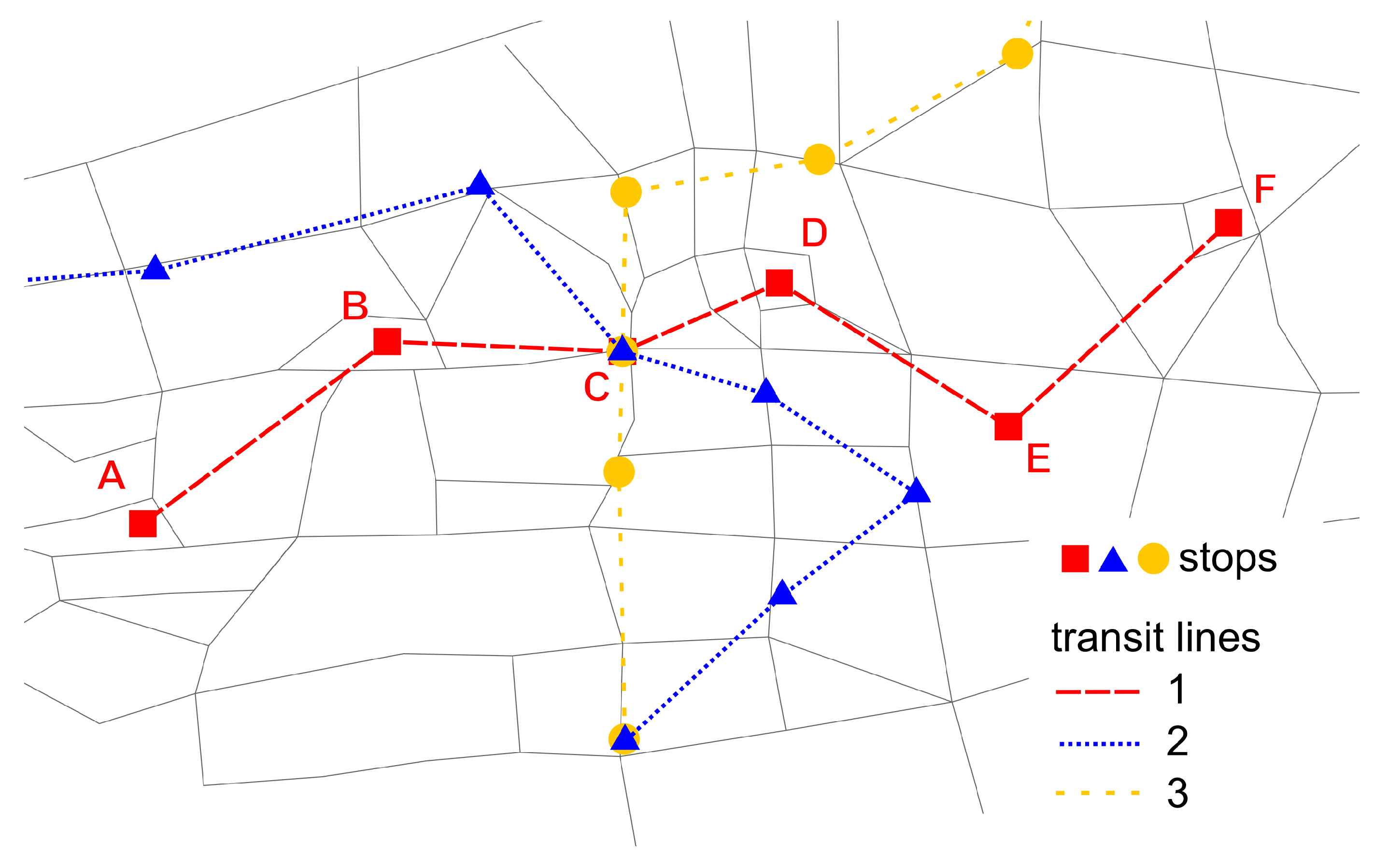
An example setup for a multimodal network is shown in Figure 1. This network will be used to illustrate the algorithm.
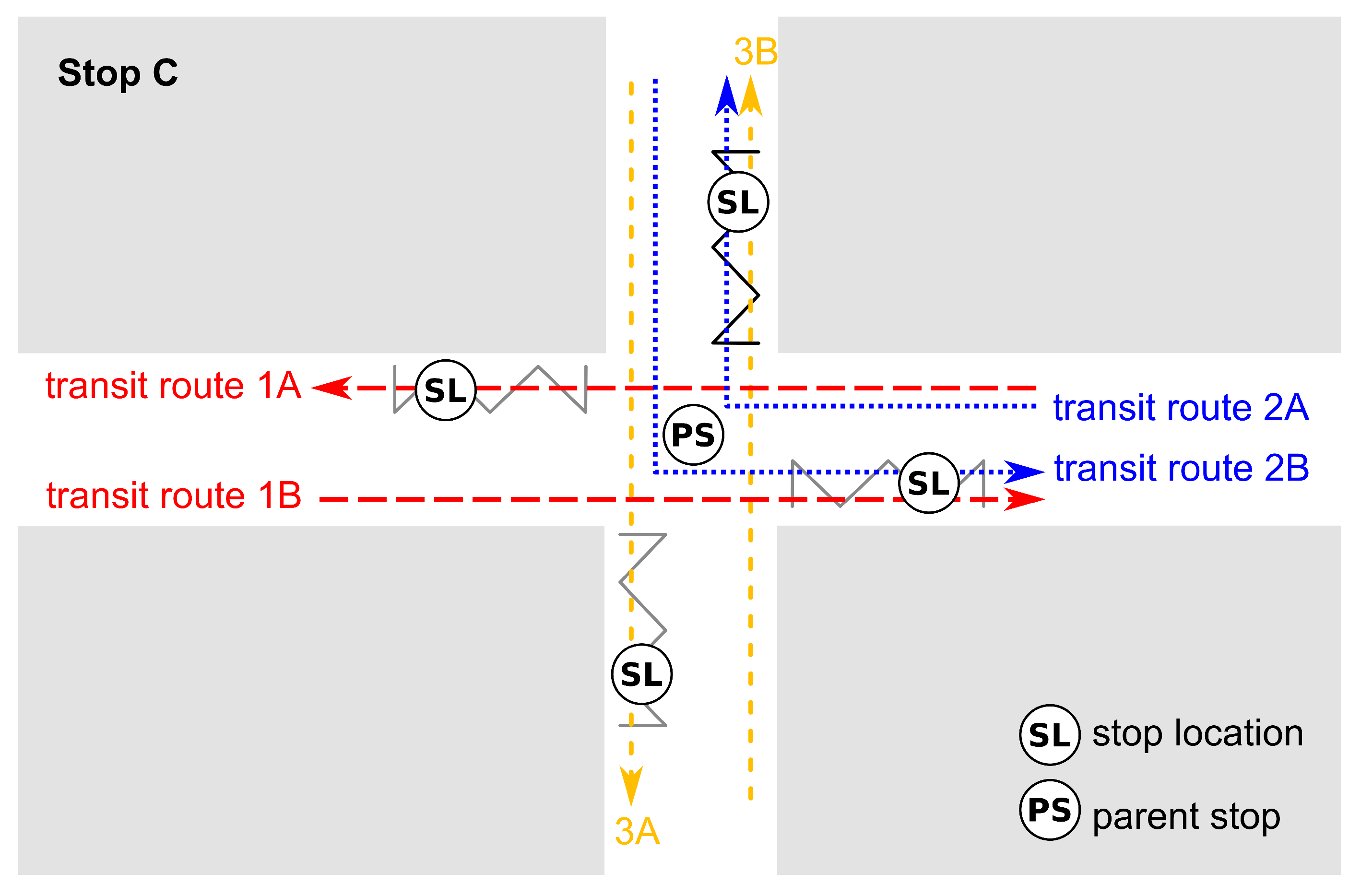
There are two types of stops that can appear in a stop sequence: stop locations or parent stops. Both are referenced with point coordinates. Figure 2 shows stop C of the example network (Figure 1) in more detail. The stop is located at an intersection and used by three bus lines. Each bus line has two transit routes. The stop has four stop locations, where the buses pick up or drop off passengers. In schedules, all four stop locations usually have the same name and are grouped to the same parent stop.
This leads to the following problem definition for finding a network path of a transit route.
A reference link for each stop, as well as the path between those referenced links must be identified. It is assumed that a public transit vehicle can access a stop by passing a link referenced to the stop. This means that a link cannot be assigned to two subsequent stops and that the network links must therefore be sufficiently short. To generate the paths, the following input data is usually available for each transit route:
- stop sequence,
- stops (either as stop locations or parent stops),
- a network as a directed graph.
The algorithm should work without using any additional GPS data.
2.2. Pseudo Routing Algorithm
The proposed version of the algorithm, the “Pseudo Routing” algorithm, requires only minimal input. It requires a schedule in which: first, each transit route has a sequence of stops and, second, each stop has coordinates. It is not required, but useful, if these stops represent stop locations instead of (generalized) parent stops. This substantially facilitates the process because stop locations inherently have only one link attached and because, usually, they have more precise coordinates closer to that link. A network is not strictly required. If no network is available, the pseudo-routing algorithm simply creates an artificial network for public transit.
The algorithm calculates the least-cost path from the transit route’s first to its last stop with the constraint that the path must contain a link candidate for every stop of the stop sequence. For each transit route, the algorithm consists of the following steps:
- Identify all possible link candidates for each stop.
- Create a pseudo graph using the link candidates as nodes. Add a dummy source and destination node to the pseudo graph.
- Calculate the least-cost path from every link candidate of a stop to every link candidate of the following stop (so called link candidate pairs). This path is represented by an edge in the pseudo graph, connecting two link candidate nodes. The edge’s weight is the path’s travel cost plus half the travel cost of the two link candidates it connects. This assures that the link candidates’ travel cost is considered too, but evenly distributed to the respective preceding and succeeding edge.
- Calculate the pseudo least-cost path from the source node to the destination node in the pseudo graph. The resulting least-cost path contains the best fit link candidate for each stop.
- Create the link sequence. Each stop is referenced to a link, which is given by the link candidate that is part of the pseudo least-cost path. The least-cost path on the real network between the referenced links is used to create the network path for the transit route.
The following explains each step in more detail.
Identify link candidates: For each stop, a set of link candidates is gathered by selecting the nearest n links from the stop’s coordinate. The link’s transport modes need to match the transport mode used by the transit route. The value of n depends on the stop coordinate and network accuracy. If both are very high (i.e., stop locations are close to the correct network link) using two link candidates, one for each direction, is enough in theory. However, in practice, using up to 10 link candidates is viable. Sometimes, no link candidates can be found because there are no links within the predefined distance (e.g., because the network model is incorrect and/or incomplete). In this case, an artificial loop link is created because all stop facilities need to be referenced to a link. This is done by adding a node to the network at the coordinates of the stop. Then, a loop link that connects this node with itself is added; this loop link is the stop’s only link candidate.
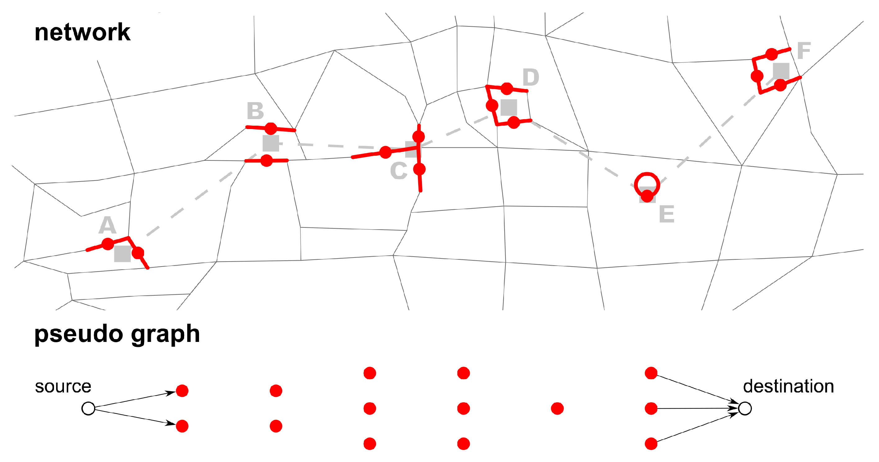
Create a pseudo graph: In the next step, the pseudo graph is initialized with each link candidate represented by a node (Figure 3). Note that these nodes do not have any actual coordinates. To efficiently calculate the least-cost path on the pseudo graph, dummy source and destination nodes are needed. The source node is connected to all link candidate nodes of the first stop, the destination node to all nodes of the last stop. All of these dummy edges have the same weight (e.g., 1).
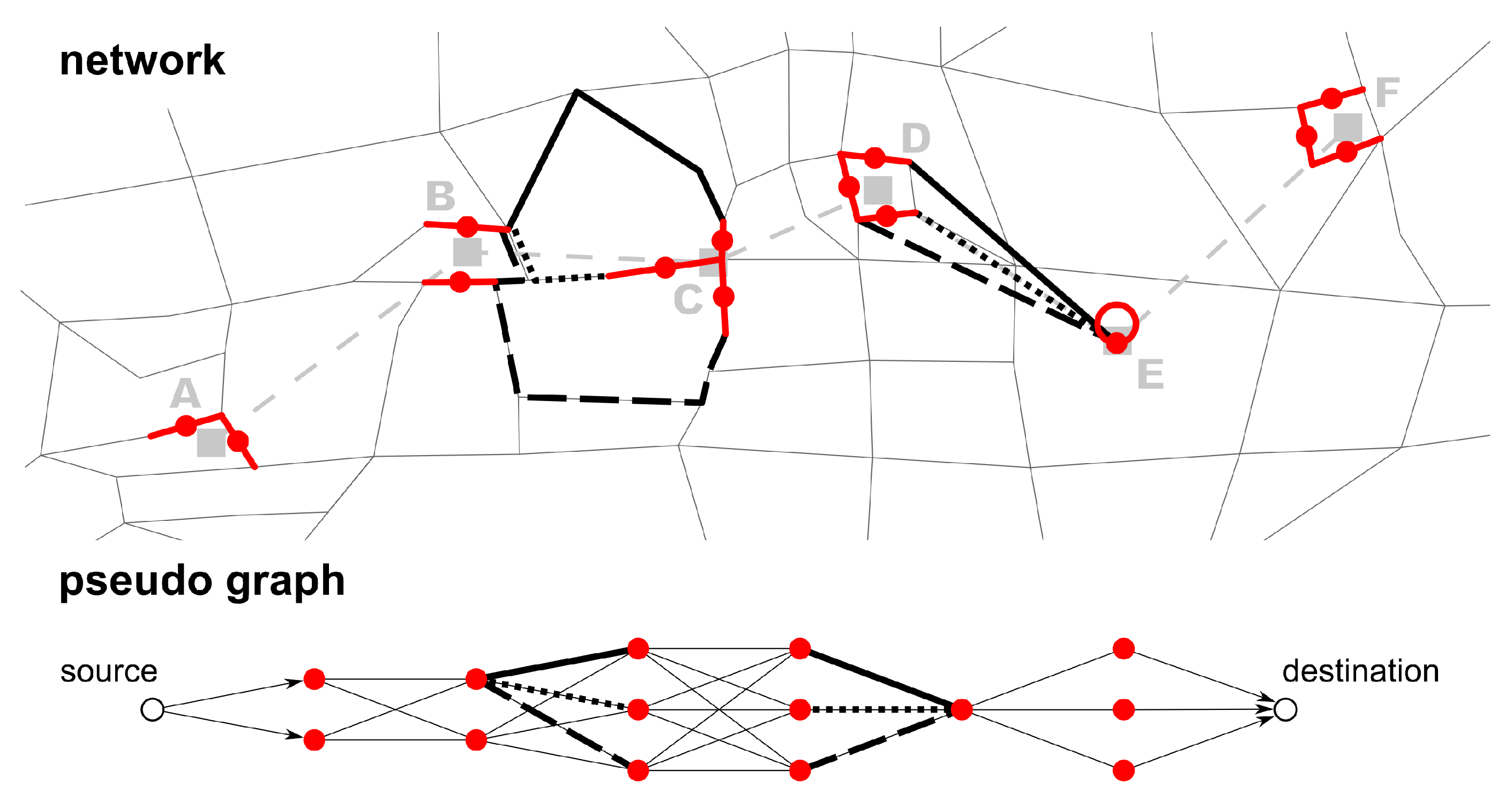
Calculate the least-cost path between each link candidate pair: in the previous step, a set of link candidates for each stop was created. These link candidates are represented as nodes in the pseudo graph. In this step, the edges of the pseudo graph are added. For each pair of link candidates of two adjacent stops, the least-cost path in the network is calculated. This path is represented by an edge in the pseudo graph (Figure 4). The pseudo edge’s weight is the path travel cost plus half the travel costs of the two link candidates the path connects. It is possible that two adjacent stops share a link candidate. As this would effectively translate to the two succeeding stops having their stop location at the same physical place, a selection of these two candidates should be prevented (see also Li [15]). This is achieved by multiplying the cost between these two candidates by four.
The travel cost on a network link is normally length or travel time, but more complex travel cost calculations are also possible. Following Ordonez and Erath [12], GPS point data or data from OSM could be included to in- or decrease the travel cost accordingly.
If no path can be found between two link candidates (e.g., because the network model is incorrect and/or incomplete), an artificial link is created and added as an edge to the pseudo graph (see Figure 4 between stops D and E). This ensures that a path can be found in the pseudo graph and thus also in the network. Artificial links can also be created if the cost of a path is greater than a defined threshold. This prevents paths with very high travel costs, which are probably incorrect. In these cases, it is very likely that a link is missing in the network model. Artificial links are not a desired output of the algorithm, but they can highlight inconsistencies in the mapping result. For this reason, an artificial link connects two link candidates directly instead of using at least some intermediate network links.
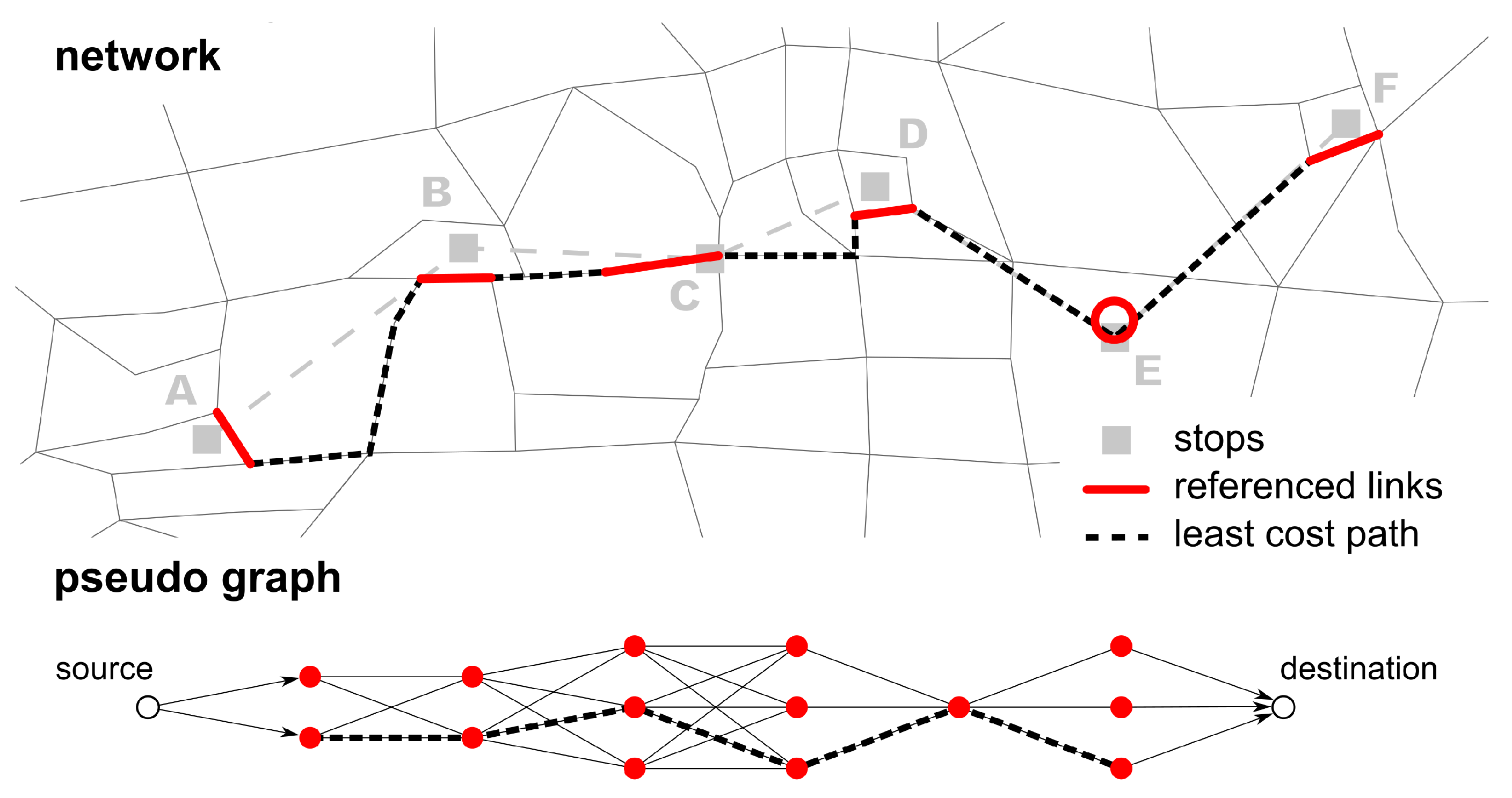
Calculate the pseudo least-cost path: The shortest path in the pseudo graph from the source node to the destination node is then calculated. Any shortest path algorithm can be used (here, a standard Dijkstra algorithm was applied). The least-cost path gives a sequence of link candidates that describes which link should be referenced to each stop of the transit route (see Figure 5).
Create the link sequence: After each stop has a link referenced, one can use the least-cost path between each reference link pair to define the path (link sequence) the vehicle takes in the network (Figure 5).
2.3. Large-Scale Networks
If the algorithm is applied to large-scale networks, line intersections happen frequently. An example for line intersections is stop C in Figure 1. The application of the algorithm to different lines might result in different stop locations for the same parent stop. This is accentuated in the case of different modes using the same parent stop (e.g., buses and ships at a harbor). This is not a mistake, but rather a correct model of reality. In contrast to other algorithms like, for example, those by Bösch and Ciari [11] or Ordonez and Erath [12], the proposed implementation of the algorithm explicitly supports multiple stop locations across different modes for the same parent stop. This is also in contrast to Li [15], as they focused on the precise identification of bus stops (see Section 1) and did not discuss this aspect.
3. Analysis
The algorithm has been implemented for MATSim [17], a multi-agent transport simulation framework, in the programming language Java. The source code is open-source (location: [16]), and Poletti [18] provides a detailed documentation of implementation. The results achieved with this algorithm implementation have been validated by testing mapping accuracy. It was also checked whether a reasonable number of stop locations was created. As a reference, the mapping implementation by Bösch and Ciari [11] was tested as well.
3.1. Reference Data
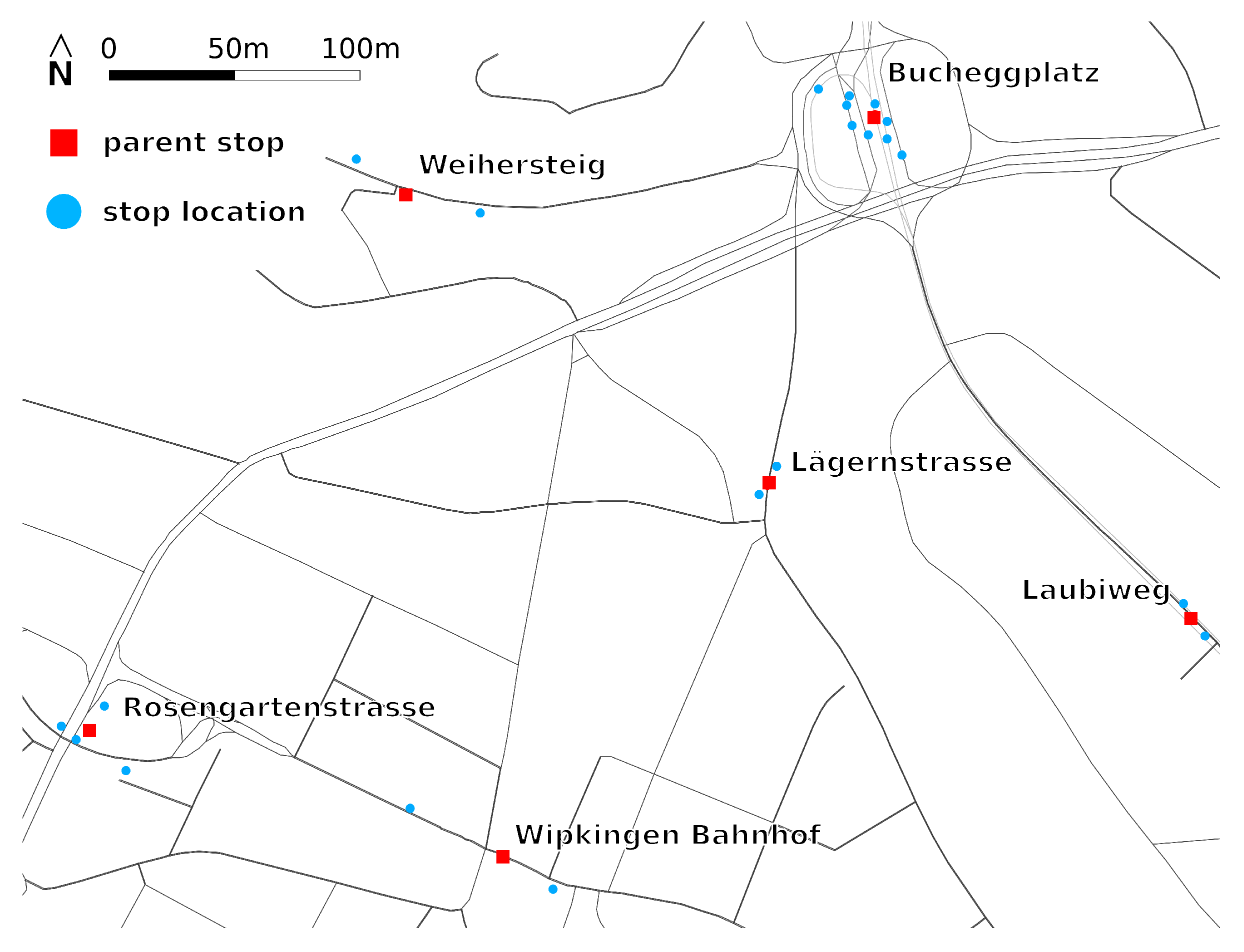
The tests were conducted with schedules based on a GTFS feed for the Zurich area [19]. The feed is provided by the Zürcher Verkehrsverbund (ZVV, Zurich transport authority) and covers all bus, tram, funicular and ferry routes of the Zurich area. There are two types of stops available: first, stop locations that are used by trips and second, parent stops which also have point coordinates, but are not accessed by any trips. Figure 6 shows an example from the feed for stop locations and parent stops. The feed also contains the shapes of the trips, i.e., geo-referenced polylines representing the PT vehicles’ routes. These shapes can be used as a source to validate the schedule created by the pseudo routing algorithm. They are available in a text file and can be converted to polylines. The feed has been converted to two unmapped MATSim transit schedules, one using stop locations as stop facilities and one using the parent stops as stop facilities. Table 1 contains descriptive information about the unmapped schedules. The unmapped schedules have been mapped to a multimodal network created from OSM (downloaded on 4 August 2016). Contrary to most traffic simulations, the links in the network were not simplified. For each stop, eight link candidates have been considered (see Section 2.2). However, links further than 80 m from a stop were not included. To see the differences to a previous approach, both schedules have also been mapped using the algorithm implemented by Bösch and Ciari [11]. Thus, four mapped schedules have been analyzed.
3.2. Number of Created Stop Locations
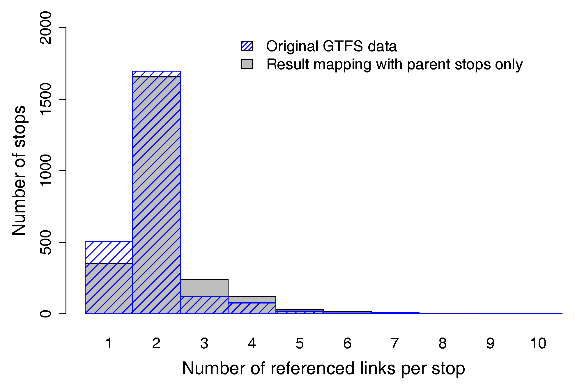
The GTFS feed differentiates between parent stops and stop locations. Thus, by comparing the original data with the mapping result, one can validate the creation of stop locations by the algorithm. Figure 7 shows the histogram of stops by the number of stop locations for the original GTFS stop locations and the artificially created stop locations.
3.3. Mapping Analysis
To test the mapping spatial validity and accuracy, generated paths from the algorithm are compared with the shapes given in the GTFS feed. The mapped routes were converted to polylines, which were compared to the trip polylines from the GTFS feed using standard Geographic Information System (GIS) software. Only bus routes were compared, since train lines are not available from the feed; tram, ferry and funicular routes are usually mapped with artificial straight links between stops. Six transit routes have been removed because the GTFS shapes were incorrect (not covering the whole trip, or straight lines from the first to the last stop). In total, 1922 transit routes were compared to their corresponding GTFS shapes.
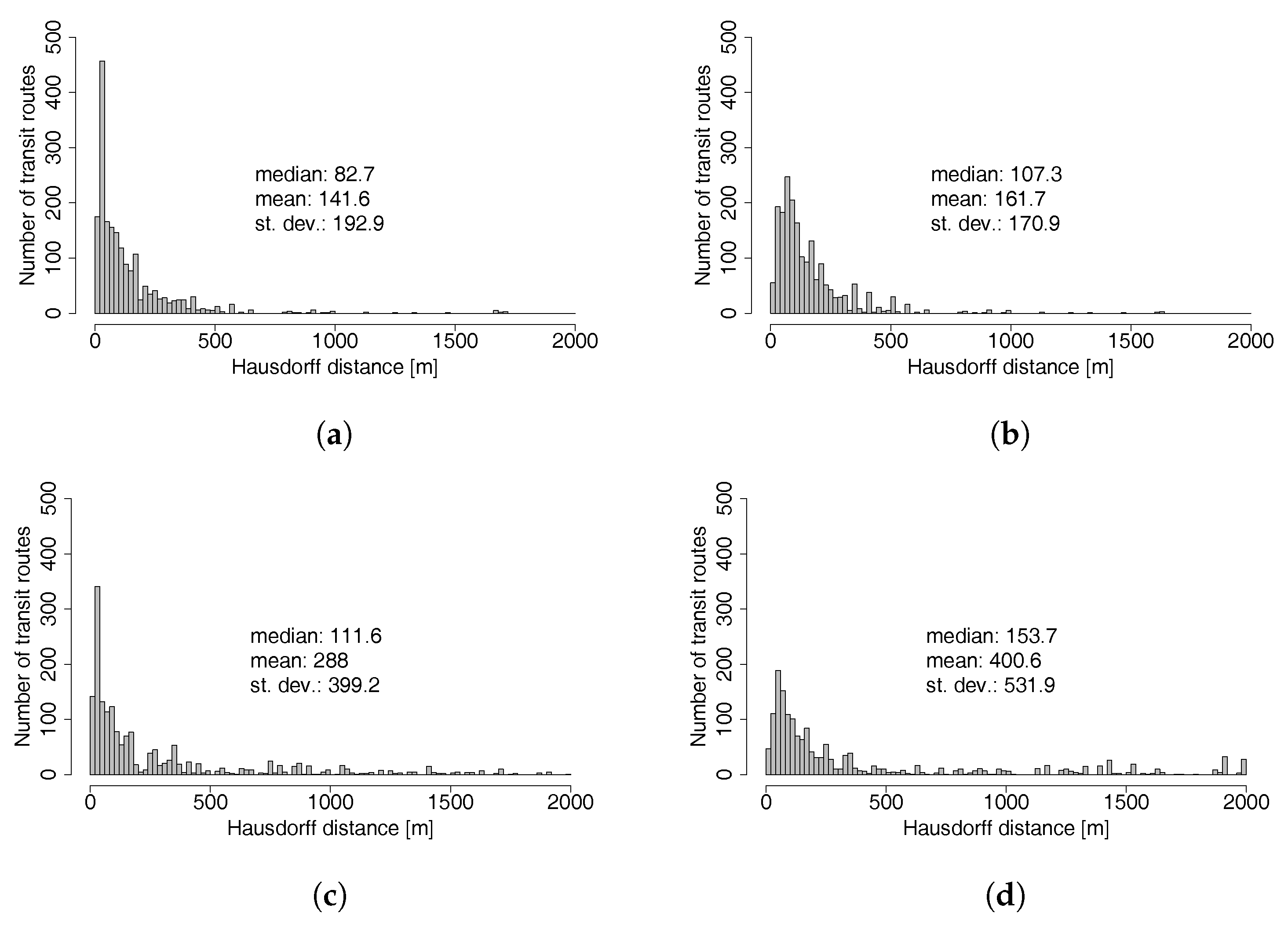
Maximal distance: A standard way to compare two geometries is the Hausdorff distance [20], which represents the greatest of all distances from a point on one line to the closest point on the other line. This single value represents the maximal distance between two lines. Figure 8 shows the Hausdorff distance between the mapped path and the GTFS path for all four mapped schedules. If the algorithm works as expected, the values should be concentrated on the left side of the graph (small maximal distances). As Figure 8 shows, this is indeed the case here, although median and mean distance values are relatively high for all of them. The new pseudo routing algorithm is performing substantially better, however, with mean and median distances considerably lower than the Bösch and Ciari [11] approach and also clearly reducing the long tail of very high distances.
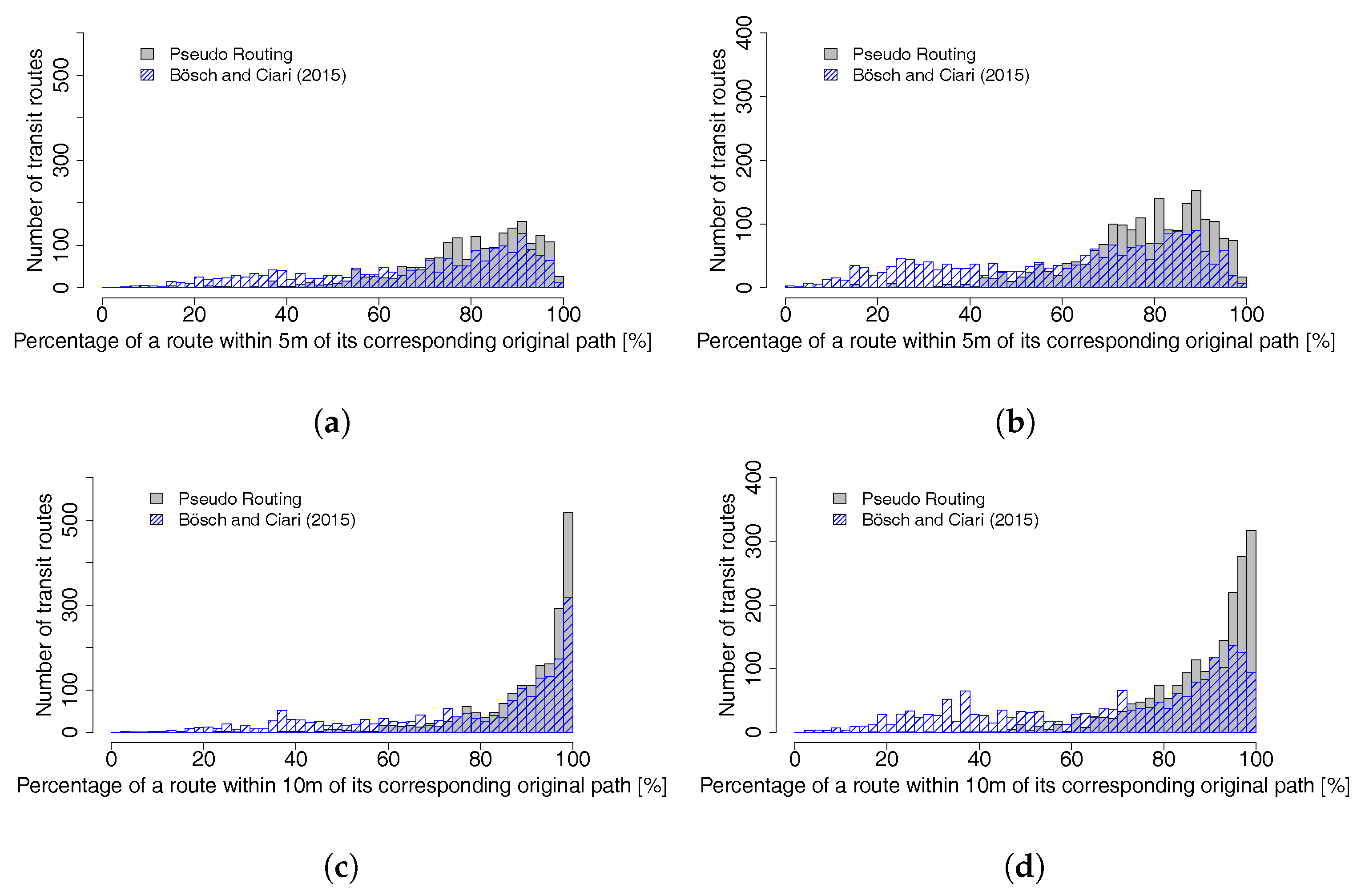
Accuracy score via buffer intersection: The Hausdorff distance does not actually quantify the similarity of two lines but is used to find most similar lines. When comparing the mapping result to the GTFS shapes, one is interested in how much of the mapped path is similar to its GTFS counterpart. To further complicate the issue, even when the mapped path is perfect, differences are to be expected because the mapping result is based on a network from OSM, which is different from the base map of the GTFS shapes. Thus, a buffer intersection test was applied; each GTFS polyline was transformed to a polygon with a buffer of 5 m or 10 m. The polyline from the mapped MATSim transit route was intersected with this buffer. This intersection defines the parts of a transit route within the buffer distance of the corresponding GTFS polyline. The accuracy score of a route is defined by the ratio of mapped path length within buffer and the total mapped path length. Figure 9 shows the score histograms for buffers of 5 and 10 m. If the algorithm is accurately generating the routes, bars will be concentrated on the right side of the graph (high overlap). In accordance with the Hausdorff results before, it is apparent that the new implementation works substantially better than the older one. The test does not clarify completely, however, if the version with stop locations or the one with parent stops is performing better. As expected, if the buffer is larger, the percentage of a route corresponding to the original path is higher.
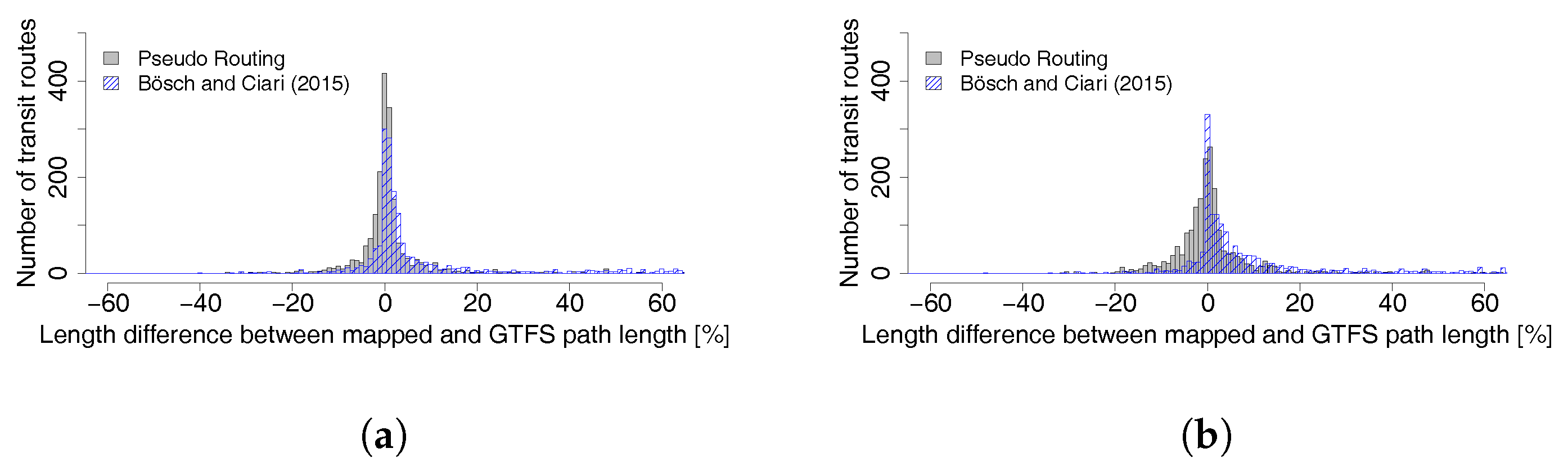
Path length difference: If a mapped transit route takes short cuts, detours, or has loops, its length will differ from the length of the GTFS line. The goal of this test is to compare the length of the GTFS path to the mapped path. Figure 10 shows the histograms for the differences between mapped path length and GTFS path length. Therefore, the more accurate the algorithm is in reproducing the original lengths, the more bars will be located in the middle of the graph. Although both implementations seem to produce fairly correct path lengths, it can again be confirmed that the new pseudo routing approach is outperforming the Bösch and Ciari [11] approach by concentrating to the center more and reducing the tail of large deviations.
4. Discussion
The test results in Section 3.2 show that the implemented pseudo routing algorithm does create a realistic number of artificial stop locations per parent stop. The number of stop locations for each parent stop is similar to the original GTFS data.
The mapping accuracy analysis (Section 3.3) shows that, overall, the majority of routes were mapped very similarly to their corresponding GTFS shapes. The accuracy score for a buffer of 10 m for both schedules (stop locations and parent stops) is satisfactory for an automatic algorithm. One should note that the test is rather simple and does not directly compare both lines, but instead the mapped path, with a general area where it should be. In addition, depending on the buffer distance, loops within the buffer cannot be detected. Manual analysis of paths with a low score showed that some were correctly mapped, but had an offset due to the different map data sources. The Hausdorff distances for all four tested schedules are higher than expected. However, this distance represents the maximal distance between two lines and the accuracy scores are relatively good. The length difference between the mapped path and the GTFS shape is very small, again for both input schedules. The implemented pseudo routing algorithm tends to give better results than the implementation by Bösch and Ciari [11] for both stop locations and parent stops.
Mapping results were not satisfying for routes whose stops are farther apart (e.g., express lines which skip some stops). If the network situation around a stop is complex (e.g., high number of links within a small radius or links on multiple street levels), it is likely that not enough link candidates are selected. This leads to incorrect paths because the right link candidates were not part of the pseudo graph. In addition, implementation might lead to unexpected results if there are too many stop facilities along a link, either because the density of stops is high or because the link is very long. Since the algorithm tries not to use the same link candidate for subsequent stops, this might lead to an invalid mapping. It should also be noted that the mapping quality largely depends on a consistent and accurate network. If links are missing (especially bus lanes), the result is likely to be wrong.
Using travel time as travel costs for the routing algorithm tends to give better results than link length. However, travel times might not work if the schedule data source uses time differences of zero between two stops.
5. Conclusions
This paper proposes an algorithm to map a public transit schedule to a network. The pseudo routing algorithm calculates the path on a network for a transit route, given its stop sequence. It calculates the least-cost path from the first to the last stop with the constraint that the path must contain a link candidate from every stop of the stop sequence. Test results show that the algorithm leads to reasonable paths and that it is a viable way to automatically generate paths for public transit vehicles in detailed large-scale models of transport networks.
The algorithm is a significant improvement over previous available algorithms of this kind. Since it copes with life scale networks, it reduces substantially, albeit not completely cancels, the manual work necessary to generate public transit networks for transportation models. This work does not have direct policy relevance. However, it provides a tool for planners and policy makers that enhances the capability of transportation models to deal in detail with public transit networks also for large scale applications. This is important given the growing emphasis given by transportation planning to multimodality; the recent success of shared mobility, its complementarity with public transit and the necessity to model them with high spatial and temporal resolution; and the possible impact of automation on public transit in the future.
There are two suggested points for future work to increase the quality of the mapping. Most problems with routes (loops or simply wrong routes) come from the wrong selection of link candidates. The proposed approach takes a number of links within a given radius. More complex link candidate search functions are conceivable: for example, depending on the number of transit routes at a stop, or on the type of stop. One could improve link candidate selection by including OSM data to order link candidates. Links that are close to a stop location identified in OSM could get a higher score. This does not even require the matching of data sets. A second improvement would be to develop more complex routers, thus improving mapping without changing the basic algorithm. Two types of link travel costs have been implemented: link length and travel time. Additional data like GPS could be included to calculate the travel cost. Links with GPS points next to them could have decreased travel costs. Again, OSM data could be included. For example, buses could have lower travel costs if they travel on links tagged as bus routes in OSM. In addition, the implemented network routers allow U-turns, which should lead to a travel cost increase in further development steps.
Acknowledgments
This research is part of the project Autonomous Cars (project number 200021_159234) funded by the Swiss National Science Foundation.
Author Contributions
F.P. and P.M.B. conceived and developed the presented algorithm and experiments; F.P. implemented the algorithm and performed the experiments; K.W.A. and F.C. supervised and supported F.P. and P.M.B.; F.P., P.M.B., F.C. and K.W.A. wrote the paper.
Conflicts of Interest
The authors declare no conflict of interest. The founding sponsors had no role in the design of the study; in the collection, analyses, or interpretation of data; in the writing of the manuscript, and in the decision to publish the results.
Abbreviations
The following abbreviations are used in this manuscript:
| GIS | Geographic information system |
| GPS | Global positioning system |
| GTFS | General transit feed specification |
| GUI | Graphical user interface |
| HAFAS | HaCon Fahrplan-Auskunfts-System |
| ID | Identifier |
| MATSim | Multi-agent transport simulation |
| OSM | Open street map |
| PS | Parent stop |
| PT | Public transit |
| SL | Stop location |
| ZVV | Zürcher Verkehrsverbund (Zurich transport authority) |
References
- Menendez, M.; Ortigosa, J.; Ambühl, L.; Axhausen, K.W.; Ciari, F.; Bösch, P.; Geroliminis, N.; Zheng, N. NetCap: Intermodale Strecken-/Linien- und Netzleistungsfähigkeit, Schlussbericht SVI 2004/032; Schriftenreihe 1563; IVT ETH Zürich und LUTS EPF Lausanne: Zurich, Switzerland, 2016. [Google Scholar]
- Loder, A.; Ambühl, L.; Menendez, M.; Axhausen, K.W. Empirics of Multimodal Traffic Networks—Using the 3D Macroscopic Fundamental Diagram; Arbeitsberichte Verkehrs- und Raumplanung 1225; IVT, ETH Zurich: Zurich, Switzerland, 2016. [Google Scholar]
- Geroliminis, N.; Zheng, N.; Ampountolas, K. A three-dimensional macroscopic fundamental diagram for mixed bi-modal urban networks. Transp. Res. Part C Emerg. Technol. 2014, 42, 168–181. [Google Scholar] [CrossRef]
- Zheng, N.; Geroliminis, N. Modeling and optimization of multimodal urban networks with limited parking and dynamic pricing. Transp. Res. Part B Methodol. 2016, 83, 36–58. [Google Scholar] [CrossRef]
- HaCon. Hafas. Available online: http://www.hacon.de/hafas/ (accessed on 26 October 2016).
- Google. What is GTFS? Available online: https://developers.google.com/transit/gtfs/ (accessed on 26 October 2016).
- Transitland. Feed Registry. Available online: https://transit.land/feed-registry/ (accessed on 26 October 2016).
- Open Street Map. The Free Wiki World Map. Available online: https://www.openstreetmap.org/ (accessed on 26 October 2016).
- Quddus, M.A.; Ochieng, W.Y.; Noland, R.B. Current map-matching algorithms for transport applications: State-of-the art and future research directions. Transp. Res. Part C Emerg. Technol. 2007, 15, 312–328. [Google Scholar] [CrossRef] [Green Version]
- Perrine, K.; Khani, A.; Ruiz-Juri, N. Map-Matching Algorithm for Applications in Multimodal Transportation Network Modeling. Transp. Res. Rec. 2015, 2537, 62–70. [Google Scholar] [CrossRef]
- Bösch, P.M.; Ciari, F. A multi-modal network for MATSim. In Proceedings of the 15th Swiss Transport Research Conference, Ascona, Switzerland, 15–17 April 2015. [Google Scholar]
- Ordonez, S.; Erath, A. Semi-Automatic Tool for Map-Matching Bus Routes on High-Resolution Navigation Networks; Technical Report; Institut für Verkehrsplanung und Transportsysteme, Eidgenössische Technische Hochschule Zürich: Zürich, Switzerland, 2011. [Google Scholar]
- Brosi, P. Real-Time Movement Visualization of Public Transit Data. Master’s Thesis, University of Freiburg, Freiburg im Breisgau, Germany, 2014. [Google Scholar]
- Geops. Mapping Public Transit Networks, 2014. Available online: http://geops.de/blog/mapping-public-transit-networks?language=en (accessed on 26 October 2016).
- Li, J.Q. Match bus stops to a digital road network by the shortest path model. Transp. Res. Part C Emerg. Technol. 2012, 22, 119–131. [Google Scholar] [CrossRef]
- MATSim Project. PT2MATSim. Available online: https://github.com/matsim-org/pt2matsim (accessed on 14 October 2016).
- Horni, A.; Nagel, K.; Axhausen, K.W. (Eds.) The Multi-Agent Transportation Simulation MATSim; Ubiquity: London, UK, 2016. [Google Scholar]
- Poletti, F. Public Transit Mapping on Multi-Modal Networks in MATSim. Master Thesis, IVT, ETH Zurich, Zurich, Switzerland, 2016. [Google Scholar]
- SBB. Offizielles Kursbuch: Fahrplandaten—Download der öffentlichen Fahrplansammlung der Schweiz. Available online: http://www.fahrplanfelder.ch/de/fahrplandaten.html (accessed on 26 October 2016).
- Huttenlocher, D.P.; Klanderman, G.A.; Rucklidge, W.J. Comparing images using the Hausdorff distance. IEEE Trans. Pattern Anal. Mach. Intell. 1993, 15, 850–863. [Google Scholar] [CrossRef]
Figure 1.
An example network containing three public transit lines: line 1 (dashed red), line 2 (dotted blue) and line 3 (dashed yellow). Line 1 is used to illustrate the mapping algorithm in Section 2.2. All transit lines have two transit routes, one going from the first to the last stop and one transit route back. Stop C is used by all three transit lines.

Figure 2.
Difference between parent stop and stop locations: stop C (see Figure 1) at an intersection is passed by three bus transit lines with two transit routes each.
Figure 2.
Difference between parent stop and stop locations: stop C (see Figure 1) at an intersection is passed by three bus transit lines with two transit routes each.

Figure 3.
Each link candidate (red) is represented as a node in the pseudo graph.

Figure 4.
The least-cost path in the network between two link candidates (top) is represented as one edge on the pseudo graph (bottom): the pseudo edge’s weight is the travel cost of the network path. Six paths and their corresponding edges on the pseudo graph are highlighted as examples.
Figure 4.
The least-cost path in the network between two link candidates (top) is represented as one edge on the pseudo graph (bottom): the pseudo edge’s weight is the travel cost of the network path. Six paths and their corresponding edges on the pseudo graph are highlighted as examples.

Figure 5.
Least-cost path from the source to the destination on the pseudo graph: The nodes of this path represent the link candidates for the stops in the network.
Figure 5.
Least-cost path from the source to the destination on the pseudo graph: The nodes of this path represent the link candidates for the stops in the network.

Figure 6.
Example for the stop locations and parent stops available in the GTFS feed for the Zurich area.
Figure 6.
Example for the stop locations and parent stops available in the GTFS feed for the Zurich area.

Figure 7.
Histogram of the number of stop locations per parent stop; original data (blue) vs. algorithm generated data (gray).
Figure 7.
Histogram of the number of stop locations per parent stop; original data (blue) vs. algorithm generated data (gray).

Figure 8.
Histogram for Hausdorff distances between the mapped transit routes and GTFS shapes. (a) pseudo routing with stop locations; (b) pseudo routing with parent stops; (c) implementation Bösch and Ciari [11] with stop locations; (d) implementation Bösch and Ciari [11] with parent stops.

Figure 9.
Histogram showing the number of transit routes for each accuracy score value. (a) schedule with stop locations, buffer 5 m; (b) schedule with parent stops, buffer 5 m; (c) schedule with stop locations, buffer 10 m; (d) schedule with parent stops, buffer 10 m.
Figure 9.
Histogram showing the number of transit routes for each accuracy score value. (a) schedule with stop locations, buffer 5 m; (b) schedule with parent stops, buffer 5 m; (c) schedule with stop locations, buffer 10 m; (d) schedule with parent stops, buffer 10 m.

Figure 10.
Histogram showing the number of transit routes for length differences in percent between the mapped transit path length and length of the corresponding GTFS path. (a) mapping with stop locations; (b) mapping with parent stops.
Figure 10.
Histogram showing the number of transit routes for length differences in percent between the mapped transit path length and length of the corresponding GTFS path. (a) mapping with stop locations; (b) mapping with parent stops.


Table 1.
Statistics on the unmapped schedules used for analysis.
| Unmapped Schedule | Unmapped Schedule | |
|---|---|---|
| Stop Locations | Parent Stops | |
| Stop facilities | 4777 | 2426 |
| Transit lines | 346 | 346 |
| Transit routes | 1928 | 1928 |
© 2017 by the authors. Licensee MDPI, Basel, Switzerland. This article is an open access article distributed under the terms and conditions of the Creative Commons Attribution (CC BY) license (http://creativecommons.org/licenses/by/4.0/).
Share and Cite
MDPI and ACS Style
Poletti, F.; Bösch, P.M.; Ciari, F.; Axhausen, K.W. Public Transit Route Mapping for Large-Scale Multimodal Networks. ISPRS Int. J. Geo-Inf. 2017, 6, 268. https://0-doi-org.brum.beds.ac.uk/10.3390/ijgi6090268
AMA Style
Poletti F, Bösch PM, Ciari F, Axhausen KW. Public Transit Route Mapping for Large-Scale Multimodal Networks. ISPRS International Journal of Geo-Information. 2017; 6(9):268. https://0-doi-org.brum.beds.ac.uk/10.3390/ijgi6090268
Chicago/Turabian StylePoletti, Flavio, Patrick M. Bösch, Francesco Ciari, and Kay W. Axhausen. 2017. "Public Transit Route Mapping for Large-Scale Multimodal Networks" ISPRS International Journal of Geo-Information 6, no. 9: 268. https://0-doi-org.brum.beds.ac.uk/10.3390/ijgi6090268
Note that from the first issue of 2016, this journal uses article numbers instead of page numbers. See further details here.