A Geometric Framework for Detection of Critical Points in a Trajectory Using Convex Hulls

Abstract

Large volumes of trajectory-based data require development of appropriate data manipulation mechanisms that will offer efficient computational solutions. In particular, identification of meaningful geometric points of such trajectories is still an open research issue. Detection of these critical points implies to identify self-intersecting, turning and curvature points so that specific geometric characteristics that are worth identifying could be denoted. This research introduces an approach called Trajectory Critical Point detection using Convex Hull (TCP-CH) to identify a minimum number of critical points. The results can be applied to large trajectory data sets in order to reduce storage costs and complexity for further data mining and analysis. The main principles of the TCP-CH algorithm include computing: convex areas, convex hull curvatures, turning points, and intersecting points. The experimental validation applied to Geolife trajectory dataset reveals that the proposed framework can identify most of intersecting points in reasonable computing time. Finally, comparison of the proposed algorithm with other methods, such as turning function shows that our approach performs relatively well when considering the overall detection quality and computing time.

1. Introduction

Nowadays, positioning data collection devices, such as GPS and wireless communication, technologies are widely available as personal devices. Users can easily record and save their geometric paths as trajectory data [1]. Trajectory data can be roughly defined as a sequence of time-stamped geographic positions of some moving objects, that is, a series of timestamped X and Y coordinates of each position. For a given trajectory T, the position of a point at a time instant i can be denoted as T(t_i). Such data can be used in many application domains, such as detection and analysis of people’s movement patterns and detection in the city, migration behavior of animals, and tracking of maritime and aerial trajectories [2,3]. The analysis of trajectories can be closely associated to the geometric, temporal, and semantic properties. Typically, the semantic dimension is related to all descriptive attributes that can be associated to a given trajectory. For instance, the series of Points Of Interest (POI) related to a given trajectory is considered as a semantic property, in which activities, mode of travel, neighbor relations, context, and any metadata during movement can be considered [4].

When considering the very large volumes of collected trajectory data often available and/or collected, the manipulation and analysis of the generated databases are not straightforward tasks [5]. Among the variety of processes that have been developed so far, clustering, Origin-Destination (O-D) methods, spatio-temporal mining, and graph-based analysis are representative trajectory analyses that have been used by previous researchers [6]. Clustering is considered as an efficient computational approach for data mining and identifying implicit geometric patterns in trajectory data [7]. The O-D methods are often apply to study the spatial and temporal distribution of start and end points of human displacements [8]. These studies apply a series of geometric-temporal and semantic criteria for the derivation of movement patterns [9]. Graph-based studies have been also applied to explore trajectory patterns [10]. A brief classification of the above methods is shown in

Table 1. Classification of trajectory-based studies.

Approach	Data Used
	GPS Data	Smart Card Data	Cell Phone Data	Other
O-D POI detection	[8,11,12,13,14]	[15]	[16]	[17]
Spatio-temporal mining	[9,14,18,19,20,21,22,23,24]	[25]	[16,26,27]	[28]
Clustering	[29,30,31,32,33,34,35]	[36,37,38]	[39,40]	[29,41,42]
Graph-based	[10,43,44]	[38]	[45,46]	[47]

according to the methods applied and data considered.

Similarity-based analysis is rather oriented to the detection of trajectory analogies and peculiarities [31]. Over the past few years, the analysis and search for similarities based on physical and geometric descriptors has been the object of several research works. According to [48], stop points provide valuable inputs for studying and differentiating trajectory data. In fact, a key issue relies on identifying effective descriptors. Events and activities that are associated to either stop points or movements also give useful insights for studying trajectory differences and similarities [49,50]. When considering geometric properties, structuring a trajectory by line segments based on curvature points has been suggested as a valuable method for identifying the main characteristics and facilitating the search for trajectory patterns [28,51,52,53,54,55]. Additional parameters such as velocity, direction, turning points and angle, acceleration, sinuosity, distance, and travel time surely provide further insights [56,57]. When considering large trajectory datasets, searching for outliers that deviate from median trajectories in both space and time has been studied in related work [19,58]. A classification of these studies according to these parameters is shown in

Table 2. Classification of parameter-based previous studies.

Property	Parameters	Related Work
Geometric	Distance	[9,10,19,27,30,31,32,34,44,45]
	Direction	[8,16,17,18,23,27,33,34,39]
	Turning Angle	[19,23,28,31]
	Sinuosity	[16,20,28,31]
Physical	Velocity	[8,18,19,27,28,44]
	Acceleration	[18,19,20]
	Stop Point	[17,18,27,30,33,34,36,43]
	POI	[9,10,14,15,16,21,22,23,24,25,30,39,40,41,42,43,44,46,47]
Context	People Attributes	[8,13,14,25,36]
	Time of Occurrence	[11,12,15,25,29,34,37,40,42,45,46]

.

An interesting quality that can be used to study the embedded properties of a trajectory is the notion of path curvature. The curvature of a given sub-trajectory can be revealed from the position of a previous point (T(P_left)) and the following one (T(P_right)), by either analyzing the rate of direction change or fitting a circle through these two given points (Figure 1).

Another descriptor that can be used when checking the similarity of some trajectories is the status of turning points [5,59]. In fact, turning points are located in the beginning and end of some trajectory curvatures. Turning points associated to a given trajectory curvature should reveal some direction changes. When searching for the geometric complexity of a given trajectory, or searching for some trajectory similarities, curvatures and turning points can play an important role. Another component that should be considered is self-intersecting trajectories. Self-intersecting trajectories arise when a given trajectory crosses its geometric path once or more. The self-intersection loops are often omitted from the geometry, although they represent some specific behaviors, like orbiting or changing the route, which have not being identified. Also, the shape of the path is sometimes intersected as the double-level intersections [19,20,28,60,61]. Figure 2 illustrates a sample of self-intersecting trajectories. This figure shows the difference between self-intersecting trajectories that can be considered as noise and should be removed (Figure 2 left) and those that represent a real sub-part of a trajectory with a self-intersecting point that is considered as a critical point in the trajectory (Figure 2 right).

One common difficulty of all the mentioned methods appears at the computational level, especially when dealing with large trajectory datasets. In order to improve processing times, a given trajectory should be filtered by keeping the most relevant points, according to the most relevant geometric descriptors. To this end, several algorithms have already been explored using spatial and temporal descriptors, such as turning points, directions, sinuosity, and speed [5,19,31]. A key issue when applying a filtering algorithm to a given trajectory is identifying the most relevant geometric descriptors, the ones that make sense with respect to the application domain considered, as well as avoiding dependent parameters. For instance, curvature and direction, as well as speed and acceleration, are dependent descriptors that should not be considered together.

The objective of this study is to develop a computational approach for identifying critical descriptors of trajectories, that is, curvature areas, turning points and self-intersecting points. A first advantage of the three selected parameters is that many other parameters, such as sinuosity, heading and curviness can be derived from curvature and turning points. As trajectories generated by most applications are very large, an important requirement is to minimize storage and computational costs, and then select the minimum number of geometrical parameters from which others can be derived. The second principle is to take into account the very specificity of urban trajectories and the fact that self-intersecting trajectories occur in many cases. As this parameter is independent of the others, it should be considered.

The proposed method follows two main objectives. The first objective is to develop a framework for identifying the minimum possible numbers of critical points and reducing the processing load of each parameter. While in previous studies, relatively costly computational processes have been implemented [61], we introduce an approach, called trajectory critical point detection using convex hull (TCP-CH), and derive our selected parameters by only using a convex hull algorithm. The application of this algorithm dramatically reduces the storage and computational costs, especially when dealing with very large trajectory datasets.

The second aim of this study is to select a few trajectory parameters that also identify the number and locations of POIs. This approach has the advantage of favoring the search for trajectory similarities when considering, for example, direction or origin-destinations. More precisely, the three selected parameters can be defined as follows:

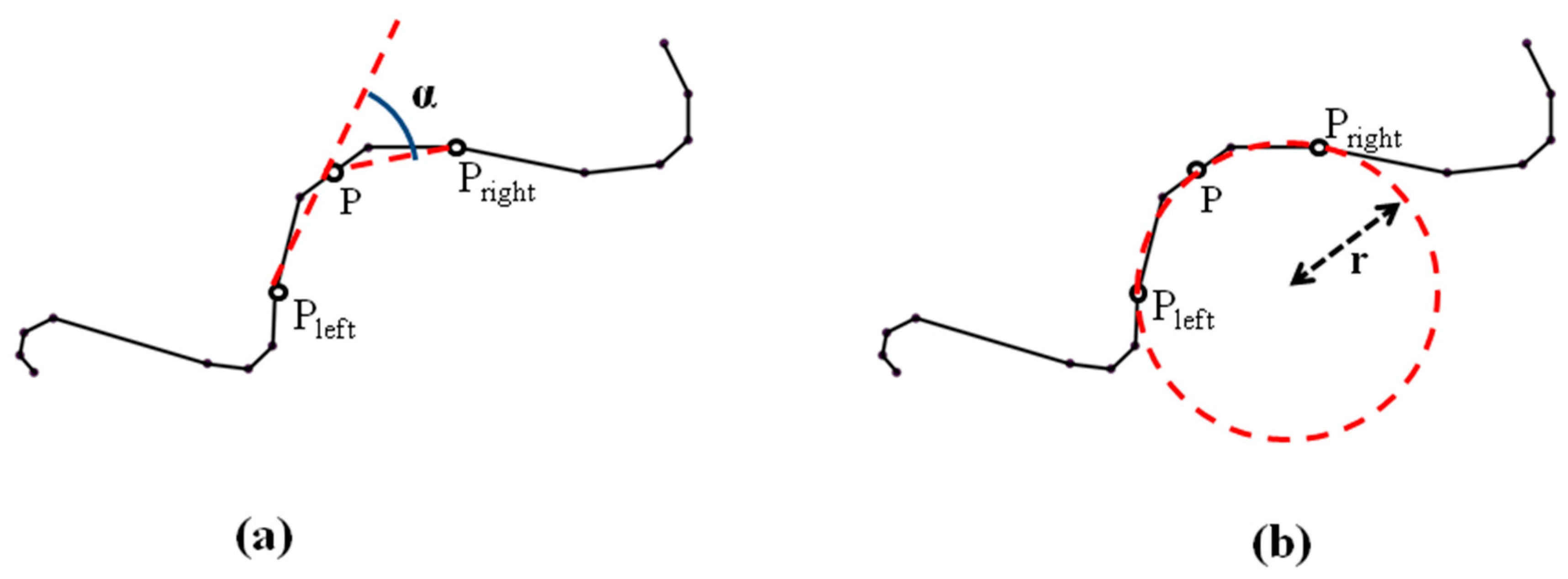
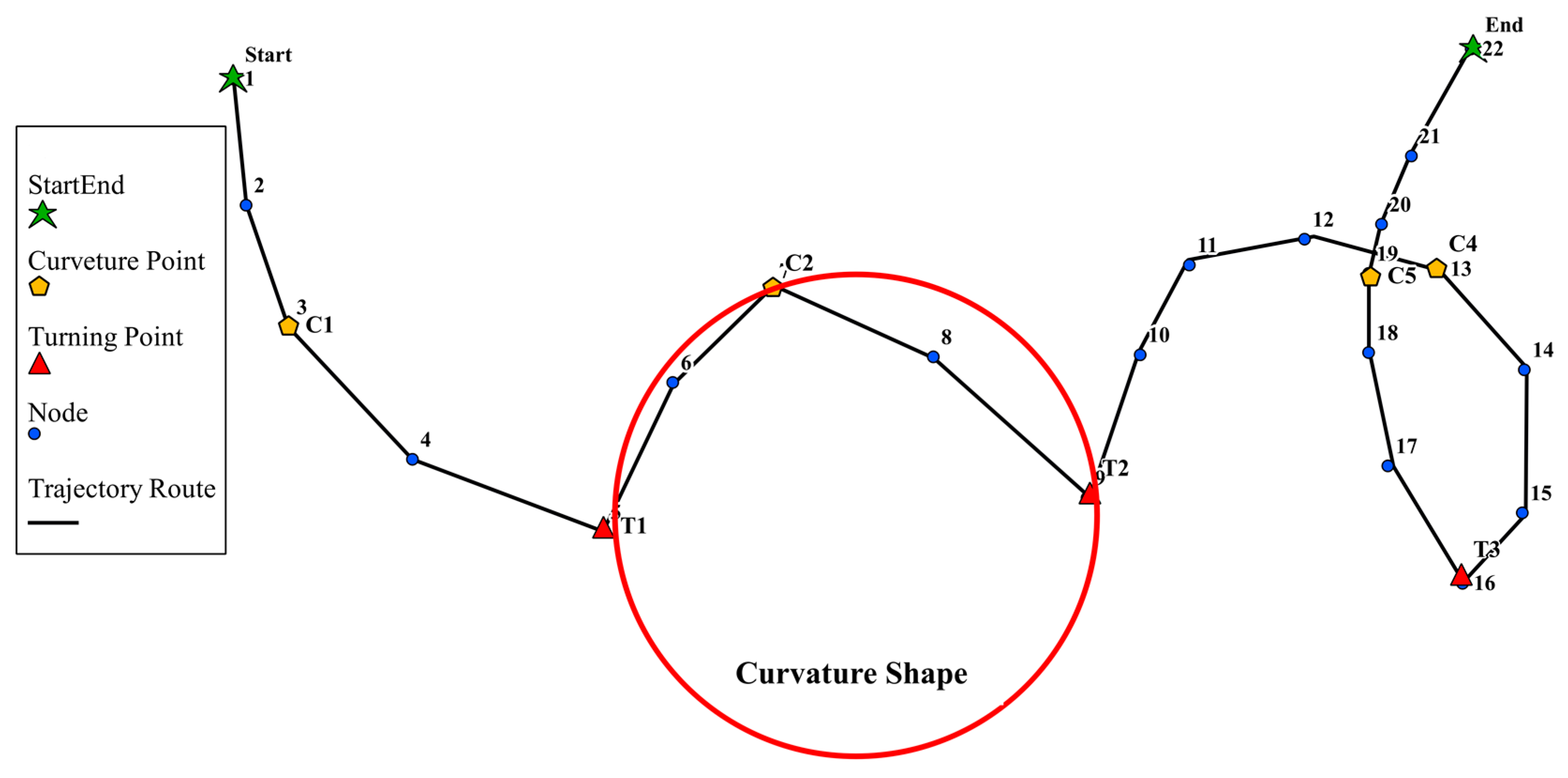
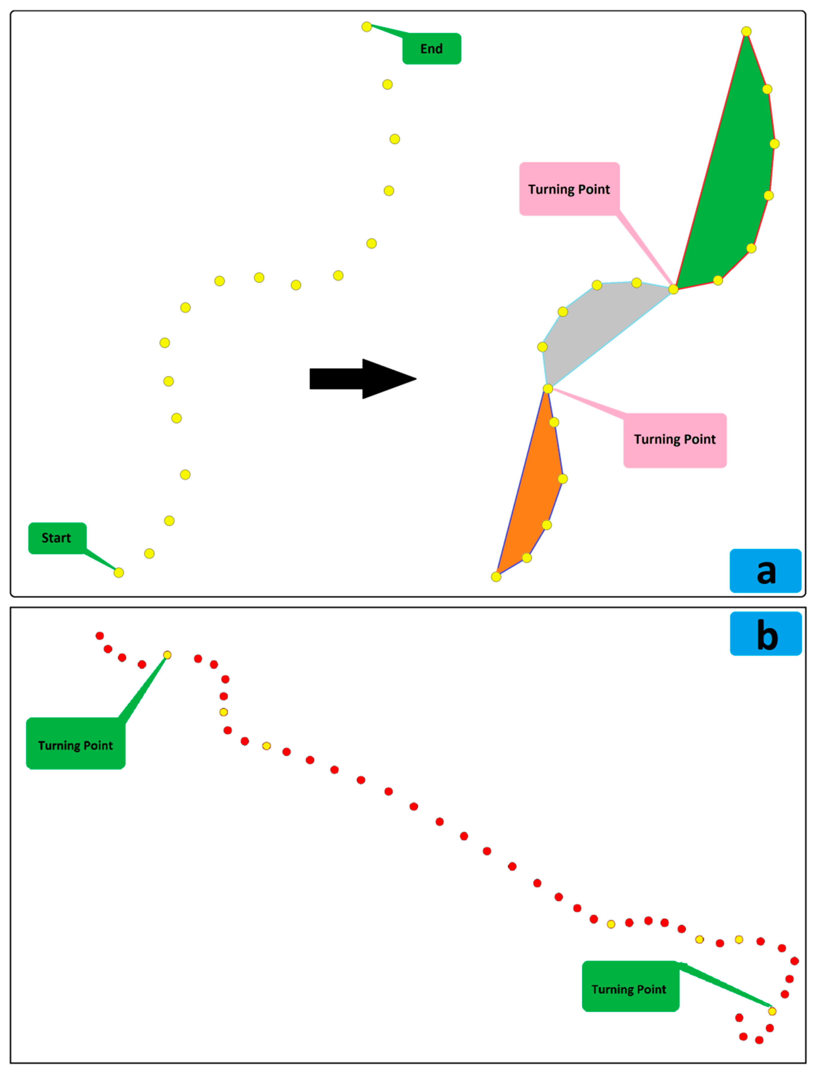
• Turning point: a turning point is considered as a changing direction point of a trajectory. For instance, a trajectory with no curve does not have any turning points, while two turning points arise for each curvature area (Figure 3).
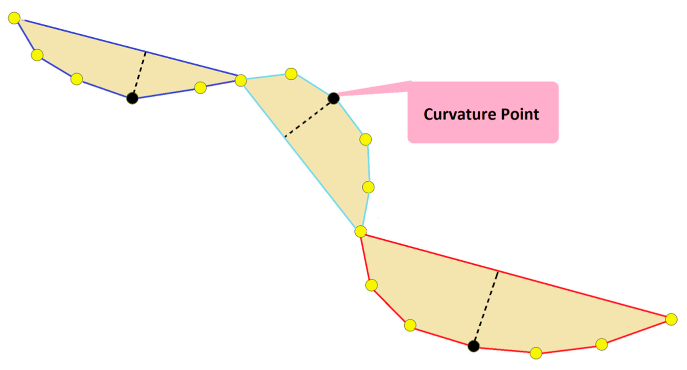
• Curvature: a curvature denotes a curve in a trajectory. Every curve has two turning points that denote the start and end of the curve, and a curvature point. A curvature can be also characterized by its length and shape (Figure 3).
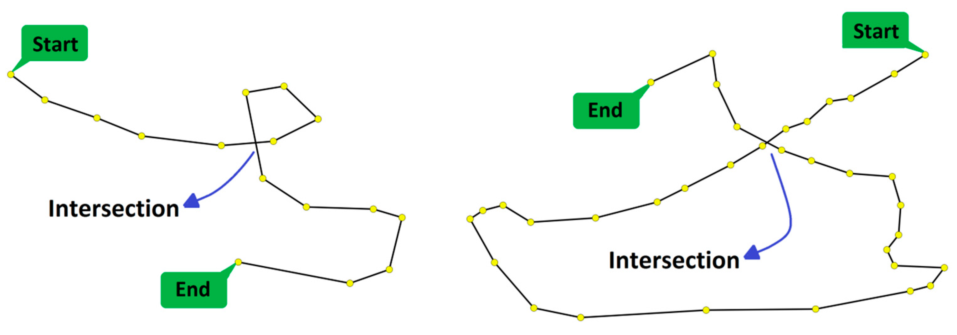
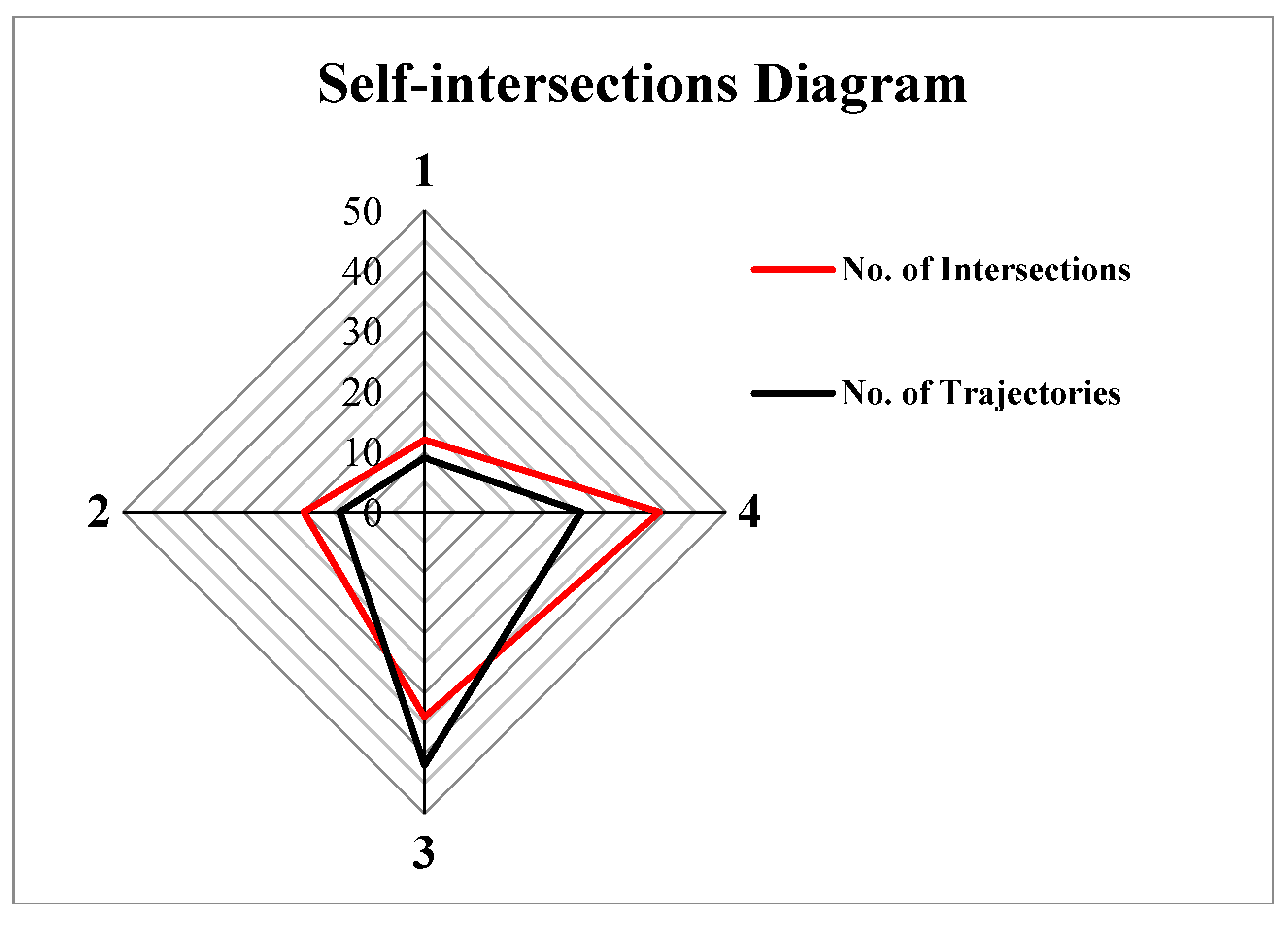
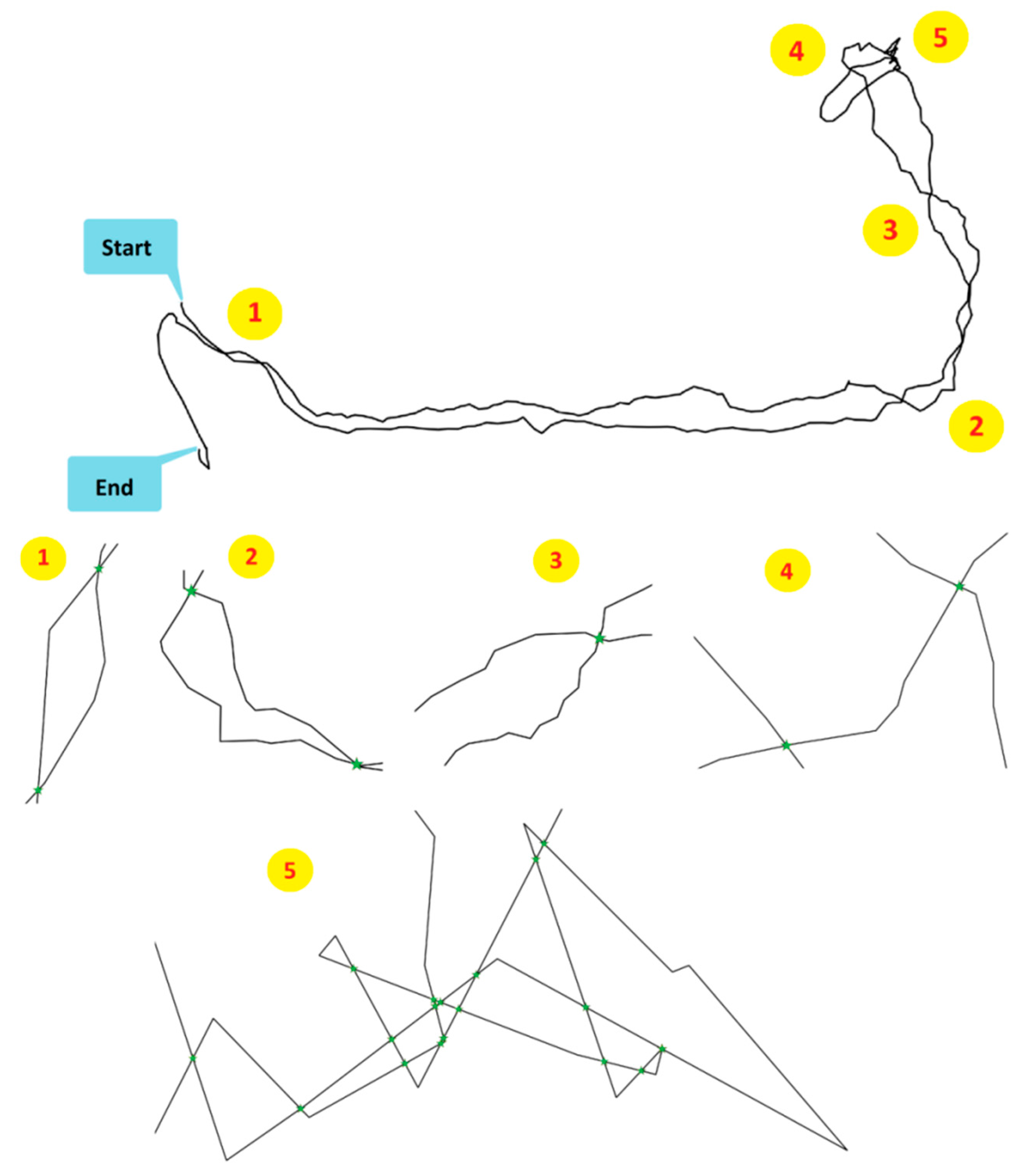
• Self-intersection point: a self-intersecting point denotes a point in the trajectories pass through at least twice. A self-interacting point is considered as a critical point as it encompasses some specific important properties: a self-intersecting point in a trajectory represents a node in the trajectory, in which the trajectory passes through twice, surely denoting the relative importance of that point. Amongst different parameters that can be considered for a self-intersecting point, the time and distance that is covered by the self-intersecting part of the trajectory can be mentioned. The role of self-intersecting trajectories has been studied in related work. For example, Keler et al. integrated 68 taxi trajectories in Shanghai to detect travel duration variety [62], while detecting 271 self-intersecting trajectories amongst 2750 intersections (Figure 4). Self-intersections are important for biological studies such as the ones applied to animal movement patterns and detection. In another related work, Bidder et al. studied horse trajectories [3], while Vrotsou et al. applied an approximation algorithm to study birds trajectories and extract movement and route patterns [63]. A few geometrical algorithms have been considered for detecting self-intersecting trajectories such as Douglas-Peucker. However, the resulting geometric simplification is not efficient enough and does not provide sufficient geometric simplification [64].

A schematic illustration of the application of these three parameters is presented in Figure 3. A convex hull algorithm is used to extract the minimum number of critical points that can be used to show all of the geometric properties of the trajectory, including shape, complexity, direction, and distance. The importance of these three parameters is to contain comprehensive information about spatial and temporal distances that can be used in geometric data mining analysis of trajectory, like pattern detection. On the other hand, it should be mentioned that other physical parameters like speed, acceleration and “stop and go” situation are also important to characterize a trajectory and search for some similarities.

The rest of the paper is organized as follows. Section 2 introduces the suggested framework for the detection of turning points and curvature areas. Section 3 presents the experimental evaluation. Finally, Section 4 concludes the paper and outlines further work.

2. Algorithm Framework

We introduced a convex hull algorithm (TCP-CH), whose objective is to detect the principal geometric characteristics according to three geometric parameters, that is, curvature, turning, and intersection points (Figure 3). Indeed, such critical points should be detected using an appropriate algorithm. The flowchart that is illustrated in Figure 5 describes the main steps of the proposed approach. First, points with inadequate spatial accuracy are omitted from movement points. These points are usually located in an illogical distance from the trend of the trajectory. The main reason that causes poor accuracy in reporting trajectory points is GPS signal as recorded by a receiver. However, in many cases, such location error at the processing phase can be solved by map matching methods [65]. The main principle behind map matching methods is to minimize the distance between the projected path on the map and the input trajectory [66,67,68]. Remaining noisy data are removed by the application of a Kalman filter to smooth the positions by recursively modifying error values. This method applies a recursive process to measurements that are observed over time (i.e., the positions coming in the GPS receiver), and predicts positions that tend to be closer to the true values of the measurements [48,69,70,71,72]. This means that after linear estimation of the points for each trajectory, the standard deviation of distance (ϭ) between two consecutive points is calculated. Next, the points with the distance higher than 2ϭ from the linear estimated model are detected as noise and are removed from the trajectory. The objective of the processing phase is to extract convex hulls as well as turning and self-intersection points from each trajectory.

2.1. Trajectory Convex Hull

One of the commonly used structures in geometric computation is the convex hull that is often considered to derive some representative geometrical structures [73]. The notion of the convex hull is widely applied in geometric computation and two-dimensional (2D) implementation of this structure was first proposed by Graham in 1972 [74]. Graham’s study acts as a foundation for geometric computation, as well as an independent domain in computer science [73]. Designing collision free paths, shape analysis, convex decomposition, and positioning are some representative examples of convex hull applications [75].

Convexity definition: a set S is a convex set if and only if any connecting line of the two points p and q of S are completely inside the set.

$$\left(\forall p,q\in S\to \overline{pq}\subseteq S\right)\leftrightarrow \mathrm{set}\mathit{s}\mathrm{is}\mathrm{convex}$$

(1)

Based on the convexity concept, a convex hull structure is a set of n points P = {p₁, p₂, …, p_n}, that is the smallest convex set containing all the points of P. Figure 6 shows a convex hull of a set from two dimension points [73,76].

Several computational methods have been suggested to derive convex hull structures. Amongst many approaches suggested so far, several approaches consider non-extreme points, extreme edges, quick hull, gift wrapping, graham, divide and conquer, and incremental [74,76,77,78]. According to the structure of trajectory data that can be considered as a time-stamped series of locations, the implementation of the proposed method is incremental. The pseudo code of the derivation of a convex hull structure using incremental method is shown in Figure 7.

The parameters of p_ih_u and p_ih_l are the connecting edges of upper and lower hulls, respectively. The incremental method divides the convex hull to upper and lower hulls as an upper hull is the part of the convex hull, which is visible from the above. It runs from its rightmost point to the leftmost point in counterclockwise order. Lower hull is the remaining part of the convex hull. The derivation of any convex hull structure in a given trajectory is based on the analysis of a sequence of points. Figure 8 shows an example of formation of four convex hulls labeled from CH₁ to CH₄ as follows: CH₁ = {p₁, p₂, p₃, p_4, p₅}, CH₂ = {p₅, p₆, p₇, p₈, p₉}, CH₃ = {p₉, p₁₀, p₁₁}, and CH₄ = {p₁₁, p₁₂, p₁₃, p₁₄, p₁₅, p₁₆} (CH is the short form of the convex hull).

2.2. Critical Points Derivation

The derivation of the critical points that act as the main descriptors of a given trajectory is based on the convex hull structure. The TCP-CH is developed hereafter. A trajectory is considered as a discrete time-stamped series of location data.

Definition 1.

A discrete trajectory T is a mapping of a time series t₁, …, t_n to the two dimension plane. For each time stamp t_i, the position (X_ti, Y_ti) in the plane is given as T(t_i). Moreover, for two given time stamps t_t and t_j with t_i < t_j, the subtrajectory T from t_i to t_j is denoted as T[t_i,t_j] [5].

Another important constraint to determine the robustness of the proposed method is the monotonicity condition, as introduced in Definition 2.

Definition 2.

A criterion is monotone if for any subtrajectory $T^{\prime }\subseteq T$, we have that if $T^{\prime }$ satisfies the criterion, then any subtrajectory $T^{″}\subseteq T^{\prime }$ also satisfies the criterion [5].

Indeed, curvature and turning points should be extracted for relevant trajectories, that is, curved trajectories. As suggested in [2], a curvature can be defined as the rate of change in the tangent vector direction of a given trajectory. A curvature can be approximated by the turning angle of the directed line segments connecting three given points (Figure 1a).

In Figure 9, an example of curved trajectory is shown. Figure 9a shows a trajectory with at least three minimum possible points that can denote a curved trajectory while Figure 9b shows a trajectory with a series of sample points recorded by GPS.

The following subsections introduce the principles of the proposed method for detecting turning, curvature, and self-intersecting points.

2.2.1. Turning Points Detection

This sub-section introduces the definition and algorithms that is applied for detecting critical turning points. In fact, a convex hull structure appears in between two sequential turning points along a given trajectory. A turning point is defined as follows:

Definition 3.

A point T(t_i) materializes a turning point for each i = 1, 2, …, n from a given trajectory n if and only if:

1. 

Conditions (2) and (3) are true for two values of j = i + 1 and s < i − 1

$$dist[\overline{T\left(t_i\right)T\left(t_{i-1}\right)},T\left(t_j\right)]>0$$

(2)

$$fors<i\to \Delta t_{i,s}isminimumanddist[\overline{T\left(t_i\right)T\left(t_{i-1}\right)},T\left(t_s\right)]\ne 0$$

(3)

2. 

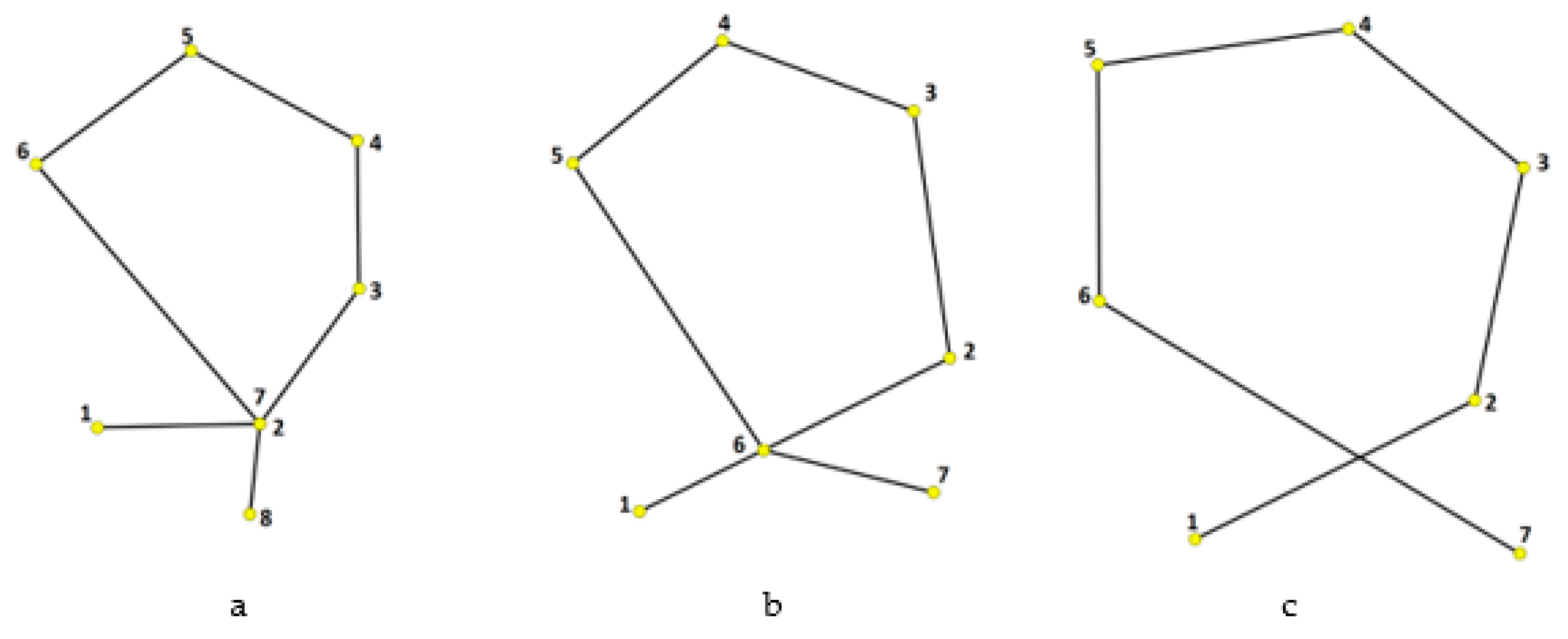
The signs of the two values extracted from Relation (4) are same and opposite to the sign of Relation (5) for two values j and s

$$\left|\begin{array}{ccc}{x}_{T\left(t_i\right)}& y_{T\left(t_i\right)}& 1\\ x_{T\left(t_{i-1}\right)}& y_{T\left(t_{i-1}\right)}& 1\\ x_{T\left(t_s\right)}& y_{T\left(t_s\right)}& 1\end{array}\right|\ne 0,\left|\begin{array}{ccc}{x}_{T\left(t_{s+1}\right)}& y_{T\left(t_{s+1}\right)}& 1\\ x_{T\left(t_s\right)}& y_{T\left(t_s\right)}& 1\\ x_{T\left(t_{s-1}\right)}& y_{T\left(t_{s-1}\right)}& 1\end{array}\right|\ne 0$$

(4)

$$\left|\begin{array}{ccc}{x}_{T\left(t_i\right)}& y_{T\left(t_i\right)}& 1\\ x_{T\left(t_{i-1}\right)}& y_{T\left(t_{i-1}\right)}& 1\\ x_{T\left(t_j\right)}& y_{T\left(t_j\right)}& 1\end{array}\right|\ne 0$$

(5)

where $x_{T\left(t_i\right)}$ and $y_{T\left(t_i\right)}$ are the coordinate specifications of the point T($t_i$) and same for the points s and j. Moreover, $dist[\overline{T\left(t_i\right)T\left(t_{i-1}\right)},T\left(t_j\right)]$ describes the distance between the connecting line of T($t_i$) and T($t_{i-1}$) to the point T($t_j$). Additionally, $\Delta t_{i,s}$ is the time difference of the points i and s. Figure 10 shows an example of trajectory with turning points. Figure 10a shows two sequential turning points, with a curvature between them. Convex hulls of a trajectory are sequentially derived as the end point of the i^th convex hull is considered as the start point for the (i + 1)^th convex hull. Figure 10b generalizes the case with a trajectory of seven turning points.

In fact, the comparison of Figure 10a and Figure 10b illustrates the monotonicity property of the application of the convex hull structure. This means that between any start and end points of a formed convex hull along a trajectory, there could not be any turning point and this feature is verified for any subset of considered convex hull points.

2.2.2. Curvature Point Detection

A critical curvature point is an important geometrical descriptor that helps to specify the shape and length of the curve. The proposed method for detecting these critical curvature points is as follows:

Definition 4.

For each point, T(t_i) and T(t_j) respectively denote the start and end points of a convex hull, while T(t_r) denotes the curvature point if and only if;

$$dist\left([\overline{T\left(t_i\right)T\left(t_j\right)}],T\left(t_r\right)\right)isMAX$$

(6)

Figure 11 illustrates the critical points of two convex hulls.

As shown in Figure 11, curvature and turning points are valuable parameters to describe the geometry of a trajectory. This also provides some useful quantifiers to evaluate the similarities between some trajectories.

2.2.3. Intersection Point Detection

Detecting the location of trajectory self-intersection is another approach for valuing and exploring possible similarities between trajectories. Indeed, self-intersecting trajectories often occur in real contexts. Detecting such trajectories allows for us to not only to simplify such trajectories, but also to qualify them. Considering discrete trajectory data—as they have been used in this study—three general modes of intersection can be defined. These three modes respectively denote Point to Point, Point to Edge and Edge to Edge cases. These three different cases are hereafter defined and illustrated in Figure 12.

Definition 5.

Point to Point mode: the points T(t_j) and T(t_i) are denoted as intersection vertices in a self-intersected trajectory if and only if for any 0 < i, r, j < n, the turning point T(t_r) exists while i < r < j and it meets the condition below:

$$T\left(t_i\right)=T\left(t_j\right)$$

(7)

Definition 6.

Point to Edge mode: the points T(t_i) and T(t_{i + 1}) are denoted as vertices of the intersection edge and T(t_s) as the intersection point if for any 0 < i, r, j < n, there exist a turning point T(t_r) while i < r < s and it meets the condition below:

$$t_i<t_s<t_{j}and\left(dist[\overline{T\left(t_i\right)T\left(t_{i+1}\right)},T\left(t_s\right)]\right)=0$$

(8)

Definition 7.

Edge to Edge mode: the two edges i and j (0 < i, j < n) contain the vertices (i, i + 1) and (j, j + 1) relatively, and are denoted as intersection edges if the line equation of these two edges intersects.

The principle behind the identification of self-intersecting points is to overlay convex hull structures.

Definition 8.

A trajectory T is a self-intersecting trajectory if and only if it meets the two conditions below:

1- 

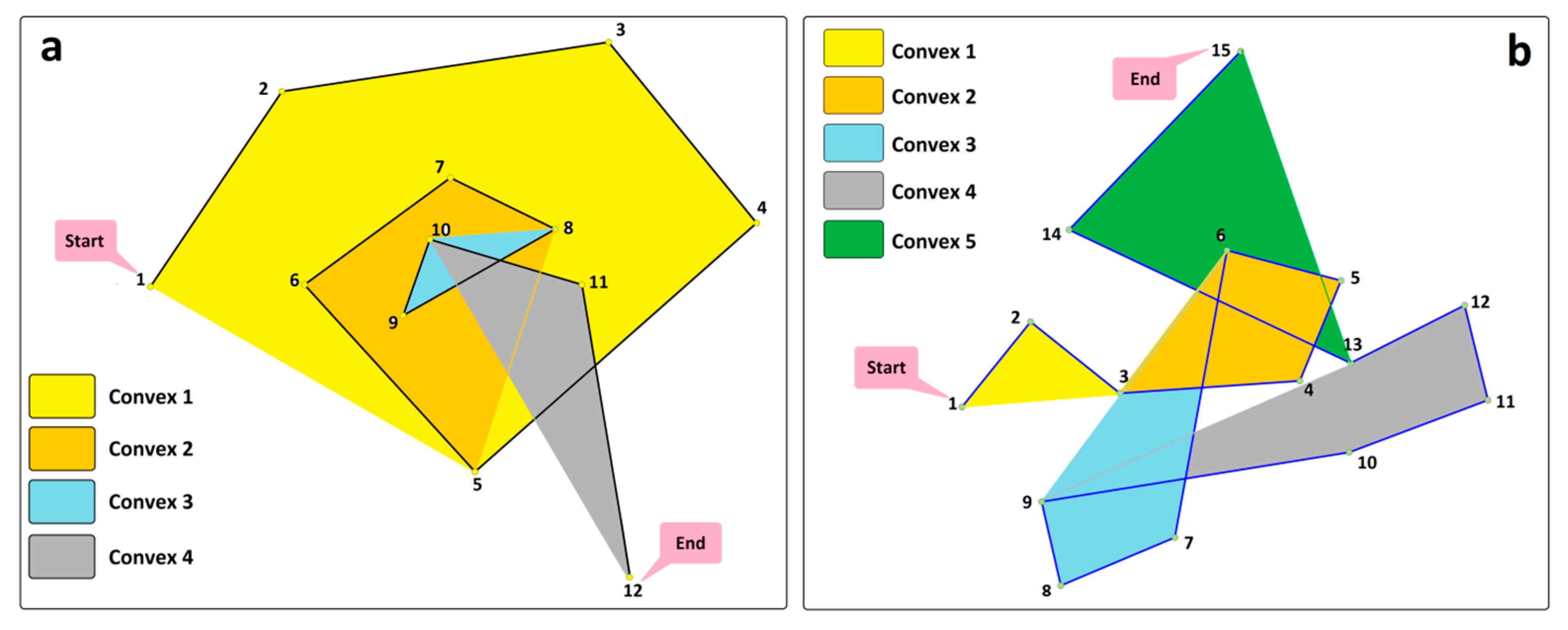
Condition 1: After derivation of convex hulls of a given trajectory, at least two convex hulls overlay.

2- 

Condition 2: For the points f and l that respectively denote the start and end points of the two convex hulls i and j, an intersection occurs between (f_i, I_i) and (f_j, I_j) if at least two edges of E_i and E_j (considering E_j є CH_i and E_j є CH_j) exist; that is, E_i is inside CH_j and E_j is inside CH_i.

The two conditions given for Definition 8 verify the existence of some self-intersection points in a given trajectory. The first condition checks whether at least two convex hulls of a trajectory overlap. This is a necessary, but not sufficient, condition when detecting self-intersecting points in a trajectory. The second condition assures the existence of intersection in trajectory data.

Figure 13 illustrates the principles applied by Definition 8. Figure 13a illustrates a subset of a trajectory with 2 self-intersections. After application of the proposed convex hull structure, 4 convex hulls are formed from points 1 to 12. These four convex hulls fulfill the first condition of Definition 8 as they overlap. However, the second condition of Definition 8 is true only between the 1st to the 4th and 3rd to the 4th convex hulls. Figure 13b provides some similar examples.

3. Implementation

The main aim of this study was to develop a computational approach for the detection of critical geometrical points of a given trajectory, namely curvature, turning and self-intersection points. This subsection describes the implementation of the different algorithms that are presented in the previous section. Figure 14 shows the sample of trajectories used in this study, which are a part of the Geolife data repository [14], which encompasses a large urban set of trajectories recorded from 2007 to 2012 by GPS devices in the city of Beijing in China.

The number of trajectories extracted from that sample equals 326, which denote travel patterns performed as walking, cycling, and by car and bus. After pre-processing and eliminating trajectory outliers, the total number of trajectory points is 83,412 and the total traveled distance is 67,2195 m. The shortest trajectory equals 8.54 m, whereas the longest one equals 14,408.2 m. Moreover, the average length of the trajectories is 2417.94 m, the average distance is 10.21 m, and the average sampling time is 5.11 s. Most of these trajectories are curved and then fulfill a necessary condition for an appropriate implementation of our algorithms. Moreover, in order to facilitate and optimize the computation of the convex hull structure, a smoothing processing step is applied to the dataset. The objective of this smoothing step is to avoid derivation of small and local convex hulls.

Table 3. Results of deleted noisy points in the trajectories.

Category	Length of Trajectory	No. of Trajectories	No. of Removed Points	Variance of Distance to Fitting Line
1	0–1000	56	63	3.41
2	1000–4000	82	235	7.33
3	4000–8000	127	1376	14.57
4	8000–15,000	61	639	17.20

shows the number of deleted noisy points at the trajectory data set divided to four groups based on length of the trajectories. The results that are presented in Table 3 show the existence of the most deviated noisy points in long-range trajectories, with the largest number of deleted points found in trajectories with lengths between 800 and 1200 m.

3.1. Detection of Curvature and Turning Points

The next step of the experimental validation is forming convex hull structures along these trajectories, as well as deriving turning and curvature points. For example, Figure 15 shows a part of trajectories 80, 125, 242, and 286, with the identified turning and curvature points. As shown in Figure 15, between two turning points, only one curvature is detected. This is an implementation confirmation of the monotonicity condition of the proposed method.

The proposed model, in addition to the detection of turning and curvature points, also dramatically decreases the number of derived points. For example, Figure 16 shows the trajectory, 80 consisting of 534 points. As shown in Figure 16, 25 critical curvature and turning points are detected, revealing the final aim of our study. In fact, the minimum meaningful number of geometric descriptors is actually derived, while largely decreasing the number of trajectory points necessary to represent the geometrical characteristics of a given trajectory.

Table 3 illustrates the overall figures of our whole implementation. Accordingly, 3253 turning points have been extracted, representing 0.045% of the input trajectory points. Our approach is compared to the one applied by [79], which takes into account a few different criteria, such as distance, direction, area, and shape. When considering our approach, the length ratio between the extract and initial trajectories is 98.1%, showing the efficiency of the algorithm in preserving the overall shape of a given trajectory. Moreover, by applying the principles that are introduced in [79], the average geometric similarity between the derived TCP-CH trajectory and the primary trajectory is 96.3% considering the parameters of distance, direction, area and shape. This reveals the high ability of the TCP-CH method in extracting critical points and keeping the primary trajectory geometry using minimum meaningful points.

One of the most important characteristics of the proposed method is computation load decrement for detecting turning points. Other methods, like turning functions, use the difference between tangent angles of the lines connecting sequential points [80]. In order to detect turning points, the mentioned method requires to derive the heading for each adjacent point, and also the difference between at least three sequential headings, thus generating computational overload and complexity. Another advantage of our proposed method is that it can detect these critical turning points only with the formation of convex hull structures along the trajectory and without heading calculation.

For a more accurate assessment of the TCP-CH method, the turning function algorithm is implemented and compared, as presented in

Table 4. Comparison of results between proposed trajectory critical point detection using convex hull (TCP-CH) method and turning function method in detecting geometric critical points.

	Data Specification	TCP-CH	Turning Function
Number of Point	73,062	3253	14,078
Mean of geometric similarity (%)	-	96.3	92.4
Length (m)	672,195.6	659,423.8	647,162.1

. As it can be seen, the turning function method has extracted 14078 points as meaningful points, which is more than four times the ones extracted by the TCP-CH method. However, the accuracy of the TCP-CH method is 3.9% higher than that of the mentioned one. Despite the large numbers of detected points by the turning function method, it is expected that the similarity accuracy also increases. This is due to the intrinsic structure of the intended method that avoids taking into account local curvatures, and, thus, preserves better accuracy. In other words, the large number of meaningful points in the turning function method generated computation overload while performing trajectory data analysis. Finally, another disadvantage of the turning function method is dependency of the accuracy of results to the data scalability. This is because some of the meaningful points at a small scale are not identifiable in large scales and vice versa. This occurs since turning function uses the angle difference of successive edges and finally, shows how the difference changes. Therefore, it falls in local differences, especially in high radius curves.

3.2. Detection of Intersection Points

The final step of this study is to identify the self-intersecting trajectories among a set of trajectory data with potential intersection points. In fact, the TCP-CH algorithm applied to the identification of self-intersecting trajectories is considered as a possible approach for the detection of trajectory similarities. Regarding the considered Geolife dataset sample, almost 17% of all data include self-intersecting trajectory points denoting 58 self-intersecting trajectories. It appears that some of these trajectories contain some simple, complex, or consecutive intersections. Furthermore, 33 trajectories have one self-intersection, while 25 trajectories have two or more intersections. In addition, the total number of intersections gives 105 self-intersection points, which can be used for trajectory similarity detection. Important aspects that are related to the analysis of these intersection points include their overall number and location (Figure 17). In this figure, the number of intersections that occurred in each quarter of trajectories is shown by the red polygon. Moreover, the number of trajectories with intersection points in each quarter is shown in Figure 17, by the black polygon. The quarter is defined based on the length of the related trajectory.

Figure 18 shows an example of a trajectory with 317 nodes and 2141 m length containing the location of several self-intersecting points, which are illustrated at a larger scale at the bottom. As shown in Figure 18, the TCP-CH algorithm method is able to derive 26 self-intersection points in total to keep the main critical points of that trajectory, while being able to properly detect these self-intersections and their positions in Section 5 by considering notable complexity.

4. Conclusions

Nowadays, in most modern cities, urban trajectory data are produced on a regular mode. This offers many opportunities for the development of data monitoring and analysis frameworks and location-based services. However, very large volumes of generated data imply to reduce the complexity and size of databases that are generated in order to decrease computation times and favor further data analysis. In particular, one common analysis developed and applied to trajectory data is to explore similarities and outliers. This implies to identify the most important and critical geometrical characteristics of some given trajectories. The research developed in this paper introduces a convex hull geometric structure, named TCP-CH, whose objective is to identify the critical points of some trajectory data. These critical points include the ones considered as such from a geometrical point of view, and in fact, the ones that can be used to characterize the geometric complexity of a given trajectory. These critical points are based on three complementary geometric descriptors including turning, curvature and self-intersection points. One of the peculiarities of the TCP-CH algorithm is that it minimizes the number of critical points that are detected for each descriptor, favoring further similarity analysis. Overall, the main advantages of the proposed method are as follows:

-

The TCP-CH method identifies critical curvature, turning and self-intersection descriptors using one common geometrical structure. In particular, we introduced a new parameter, named self-intersection, which improves the accuracy of trajectory similarity detection.

-

These critical points favor the generalization of derived trajectory that keeps the main and the most valuable geometrical characteristics of a given trajectory with sufficient accuracy. Overall, the TCP-CH method exhibits more than 96% of similarity when evaluating distance, area, direction, and shape parameters.

-

Comparison of the TCP-CH method with the turning function method—which is a common method applied for the detection of curvatures—shows more than 3% accuracy improvement when considering that the number of detected critical points is four times less than the mentioned method.

Overall, the TCP-CH method provides a framework that can be used for the analysis of geometrical trajectories, regardless of the domain of study. Indeed, the examples that are developed in this paper are closely related to urban trajectories; however, many other domains of application might be also explored with additional geometrical characteristics. Furthermore, despite the fact that the contribution is extremely limited to the spatial dimension, integration of additional semantic and temporal parameters might provide additional information and data inputs that can surely enrich and extend the applicability of our whole approach.

References

1. Zhao, P.; Qin, K.; Ye, X.; Wang, Y.; Chen, Y. A trajectory clustering approach based on decision graph and data field for detecting hotspots. Int. J. Geogr. Inf. Sci. 2016, 31, 1–27. [Google Scholar] [CrossRef]
2. Bertrand, F.; Bouju, A.; Claramunt, C.; Devogele, T.; Ray, C. Web architecture for monitoring and visualizing mobile objects in maritime contexts. In Proceedings of the International Symposium on Web and Wireless Geographical Information Systems, Cardiff, UK, 28–29 November 2007; Springer: Berlin, Germany. [Google Scholar]
3. Bidder, O.; Walker, J.; Jones, M.; Holton, M.; Urge, P.; Scantlebury, D.; Marks, N.; Magowan, E.; Maguire, I.; Wilson, R. Step by step: Reconstruction of terrestrial animal movement paths by dead-reckoning. Mov. Ecol. 2015, 3, 23. [Google Scholar] [CrossRef] [PubMed] [Green Version]
4. Bogorny, V.; Renso, C.; Aquino, A.R.; Lucca Siqueira, F.; Alvares, L.O. CONSTAnT—A conceptual data model for semantic trajectories of moving objects. Trans. GIS 2014, 18, 66–88. [Google Scholar] [CrossRef]
5. Buchin, M.; Driemel, A.; van Kreveld, M.; Sacristán, V. Segmenting trajectories: A framework and algorithms using spatiotemporal criteria. J. Spat. Inf. Sci. 2011, 2011, 33–63. [Google Scholar]
6. Sadahiro, Y.; Lay, R.; Kobayashi, T. Trajectories of moving objects on a network: Detection of similarities, visualization of relations, and classification of trajectories. Trans. GIS 2013, 17, 18–40. [Google Scholar] [CrossRef]
7. Izakian, Z.; Mesgari, M.S.; Abraham, A. Automated clustering of trajectory data using a particle swarm optimization. Comput. Environ. Urban Syst. 2016, 55, 55–65. [Google Scholar] [CrossRef]
8. Lu, M.; Wang, Z.; Liang, J.; Yuan, X. OD-Wheel: Visual design to explore OD patterns of a central region. In Proceedings of the 2015 IEEE Pacific Visualization Symposium (PacificVis), Hangzhou, China, 14–17 April 2015. [Google Scholar]
9. Cao, H.; Mamoulis, N.; Cheung, D.W. Mining frequent spatio-temporal sequential patterns. In Proceedings of the Fifth IEEE International Conference on Data Mining, Houston, TX, USA, 27–30 November 2005. [Google Scholar]
10. El Mahrsi, M.K.; Rossi, F. Graph-based approaches to clustering network-constrained trajectory data. In Proceedings of the International Workshop on New Frontiers in Mining Complex Patterns, Bristol, UK, 24 September 2012; Springer: Berlin, Germany, 2012. [Google Scholar]
11. Jiang, X.; Zheng, C.; Tian, Y.; Liang, R. Large-scale taxi o/d visual analytics for understanding metropolitan human movement patterns. J. Vis. 2015, 18, 185–200. [Google Scholar] [CrossRef]
12. Tang, J.; Liu, F.; Wang, Y.; Wang, H. Uncovering urban human mobility from large scale taxi GPS data. Phys. A Stat. Mech. Appl. 2015, 438, 140–153. [Google Scholar] [CrossRef]
13. Hanaoka, K.; Nakaya, T.; Yano, K.; Inoue, S. Network-based spatial interpolation of commuting trajectories: Application of a university commuting management project in Kyoto, Japan. J. Transp. Geogr. 2014, 34, 274–281. [Google Scholar] [CrossRef]
14. Zheng, Y.; Zhang, L.; Xie, X.; Ma, W.Y. Mining interesting locations and travel sequences from GPS trajectories. In Proceedings of the 18th International Conference on World Wide Web, Madrid, Spain, 20–24 April 2009; ACM: New York, NY, USA, 2009. [Google Scholar]
15. Chapleau, R.; Chu, K.K.A. Modeling transit travel patterns from location-stamped smart card data using a disaggregate approach. In Proceedings of the 11th World Conference on Transport Research, Berkeley, CA, USA, 24–28 June 2007. [Google Scholar]
16. Aung, S.S.; Naing, T.T. Mining Data for Traffic Detection System Using GPS _enable Mobile Phone in Mobile Cloud Infrastructure. Int. J. Cloud Comput. Serv. Archit. 2014, 4, 1–12. [Google Scholar]
17. Perttunen, M.; Kostakos, V.; Riekki, J.; Ojala, T. Urban traffic analysis through multi-modal sensing. Pers. Ubiquitous Comput. 2015, 19, 709–721. [Google Scholar] [CrossRef]
18. Zheng, Y.; Chen, Y.; Li, Q.; Xie, X.; Ma, W.Y. Understanding transportation modes based on GPS data for web applications. ACM Trans. Web 2010, 4, 1. [Google Scholar] [CrossRef]
19. Dodge, S.; Weibel, R.; Forootan, E. Revealing the physics of movement: Comparing the similarity of movement characteristics of different types of moving objects. Comput. Environ. Urban Syst. 2009, 33, 419–434. [Google Scholar] [CrossRef] [Green Version]
20. Dodge, S.; Weibel, R.; Laube, P. Trajectory similarity analysis in movement parameter space. In Proceedings of the GIS Research UK Annual Conference, Plymouth, UK, 27–29 April 2011. [Google Scholar]
21. Cao, H.; Mamoulis, N.; Cheung, D.W. Discovery of periodic patterns in spatiotemporal sequences. IEEE Trans. Knowl. Data Eng. 2007, 19, 453–467. [Google Scholar] [CrossRef]
22. Lin, M.; Hsu, W.-J.; Lee, Z.Q. Predictability of individuals’ mobility with high-resolution positioning data. In Proceedings of the 2012 ACM Conference on Ubiquitous Computing, Pittsburgh, PA, USA, 5–8 September 2012; ACM: New York, NY, USA, 2012. [Google Scholar]
23. Monreale, A.; Pinelli, F.; Trasarti, R.; Giannotti, F. Wherenext: A location predictor on trajectory pattern mining. In Proceedings of the 15th ACM SIGKDD International Conference on Knowledge Discovery and Data Mining, Paris, France, 28 June–1 July 2009; ACM: New York, NY, USA, 2009. [Google Scholar]
24. Han, J.; Dong, G.; Yin, Y. Efficient mining of partial periodic patterns in time series database. In Proceedings of the 15th IEEE International Conference on Data Engineering, Sydney, Australia, 23–26 March 1999. [Google Scholar]
25. Gong, Y.; Liu, Y.; Lin, Y.; Yang, J.; Duan, Z.; Li, G. Exploring spatiotemporal characteristics of intra-urban trips using metro smartcard records. In Proceedings of the 20th IEEE International Conference on Geoinformatics, Hong Kong, China, 15–17 June 2012. [Google Scholar]
26. Widhalm, P.; Yang, Y.; Ulm, M.; Athavale, S.; González, M.C. Discovering urban activity patterns in cell phone data. Transportation 2015, 42, 597–623. [Google Scholar] [CrossRef]
27. Asakura, Y.; Hato, E. Tracking survey for individual travel behaviour using mobile communication instruments. Transp. Res. Part C Emerg. Technol. 2004, 12, 273–291. [Google Scholar] [CrossRef]
28. Soleymani, A.; Cachat, J.; Robinson, K.; Dodge, S.; Kalueff, A.; Weibel, R. Integrating cross-scale analysis in the spatial and temporal domains for classification of behavioral movement. J. Spat. Inf. Sci. 2014, 2014, 74. [Google Scholar] [CrossRef]
29. Lee, J.-G.; Han, J.; Whang, K.-Y. Trajectory clustering: A partition-and-group framework. In Proceedings of the 2007 ACM SIGMOD International Conference on Management of data, Beijing, China, 11–14 June 2007; ACM: New York, NY, USA, 2007. [Google Scholar]
30. Lee, J.-G.; Han, J.; Li, X.; Cheng, H. Mining discriminative patterns for classifying trajectories on road networks. IEEE Trans. Knowl. Data Eng. 2011, 23, 713–726. [Google Scholar] [CrossRef]
31. Lin, M.; Hsu, W.-J. Mining GPS data for mobility patterns: A survey. Pervasive Mob. Comput. 2014, 12, 1–16. [Google Scholar] [CrossRef]
32. Morzy, M. Mining frequent trajectories of moving objects for location prediction. In Proceedings of the Machine Learning and Data Mining in Pattern Recognition, Leipzig, Germany, 18–20 July 2007; pp. 667–680. [Google Scholar]
33. Lee, J.-G.; Han, J.; Li, X.; Gonzalez, H. TraClass: Trajectory classification using hierarchical region-based and trajectory-based clustering. Proc. VLDB Endow. 2008, 1, 1081–1094. [Google Scholar] [CrossRef]
34. Pelekis, N.; Kopanakis, I.; Kotsifakos, E.; Frentzos, E.; Theodoridis, Y. Clustering trajectories of moving objects in an uncertain world. In Proceedings of the Ninth IEEE International Conference on Data Mining, Miami, FL, USA, 6–9 December 2009. [Google Scholar]
35. Nanni, M.; Pedreschi, D. Time-focused clustering of trajectories of moving objects. J. Intell. Inf. Syst. 2006, 27, 267–289. [Google Scholar] [CrossRef]
36. Hofmann, M.; Wilson, S.P.; White, P. Automated identification of linked trips at trip level using electronic fare collection data. In Proceedings of the 88th Annual Meeting on Transportation Research Board, Washington, DC, USA, 11–15 January 2009. [Google Scholar]
37. Morency, C.; Trépanier, M.; Agard, B. Analysing the variability of transit users behaviour with smart card data. In Proceedings of the IEEE Intelligent Transportation Systems Conference, Toronto, ON, Canada, 17–20 September 2006. [Google Scholar]
38. Pelletier, M.-P.; Trépanier, M.; Morency, C. Smart card data use in public transit: A literature review. Transp. Res. Part C Emerg. Technol. 2011, 19, 557–568. [Google Scholar] [CrossRef]
39. Gao, S.; Liu, Y.; Wang, Y.; Ma, X. Discovering spatial interaction communities from mobile phone data. Trans. GIS 2013, 17, 463–481. [Google Scholar] [CrossRef]
40. Zhang, Y.; Qin, X.; Dong, S.; Ran, B. Daily OD matrix estimation using cellular probe data. In Proceedings of the 89th Annual Meeting Transportation Research Board, Washington, DC, USA, 10–14 January 2010. [Google Scholar]
41. Crandall, D.J.; Backstrom, L.; Huttenlocher, D.; Kleinberg, J. Mapping the world’s photos. In Proceedings of the 18th International Conference on World Wide Web, Madrid, Spain, 20–24 April 2009; ACM: New York, NY, USA, 2009. [Google Scholar]
42. Fujisaka, T.; Lee, R.; Sumiya, K. Exploring urban characteristics using movement history of mass mobile microbloggers. In Proceedings of the Eleventh Workshop on Mobile Computing Systems and Applications, Annapolis, MD, USA, 22–23 February 2010; ACM: New York, NY, USA, 2010. [Google Scholar]
43. Zhou, Y.; Fang, Z.; Thill, J.-C.; Li, Q.; Li, Y. Functionally critical locations in an urban transportation network: Identification and space–time analysis using taxi trajectories. Comput. Environ. Urban Syst. 2015, 52, 34–47. [Google Scholar] [CrossRef]
44. Fang, H.; Hsu, W.-J.; Rudolph, L. Mining user position log for construction of personalized activity map. In Proceedings of the International Conference on Advanced Data Mining and Applications, Beijing, China, 17–19 August 2009; Springer: Berlin, Germany, 2009. [Google Scholar]
45. Gonzalez, M.C.; Hidalgo, C.A.; Barabasi, A.-L. Understanding individual human mobility patterns. Nature 2008, 453, 779–782. [Google Scholar] [CrossRef] [PubMed]
46. Ratti, C.; Frenchman, D.; Pulselli, R.M.; Williams, S. Mobile landscapes: Using location data from cell phones for urban analysis. Environ. Plan. B Plan. Des. 2006, 33, 727–748. [Google Scholar] [CrossRef]
47. Brockmann, D.; Theis, F. Money circulation, trackable items, and the emergence of universal human mobility patterns. IEEE Pervasive Comput. 2008, 7. [Google Scholar] [CrossRef]
48. Parent, C.; Spaccapietra, S.; Renso, C.; Andrienko, G.; Andrienko, N.; Bogorny, V.; Damiani, M.L.; Gkoulalas-Divanis, A.; Macedo, J.; Pelekis, N. Semantic trajectories modeling and analysis. ACM Comput. Surv. 2013, 45, 42. [Google Scholar] [CrossRef]
49. Hornsby, K.S.; Cole, S. Modeling Moving Geospatial Objects from an Event-based Perspective. Trans. GIS 2007, 11, 555–573. [Google Scholar] [CrossRef]
50. Robinson, A.C.; Peuquet, D.J.; Pezanowski, S.; Hardisty, F.A.; Swedberg, B. Design and evaluation of a geovisual analytics system for uncovering patterns in spatio-temporal event data. Cartogr. Geogr. Inf. Sci. 2017, 44, 216–228. [Google Scholar] [CrossRef]
51. Bashir, F.I.; Khokhar, A.A.; Schonfeld, D. Object trajectory-based activity classification and recognition using hidden Markov models. IEEE Trans. Image Process. 2007, 16, 1912–1919. [Google Scholar] [CrossRef] [PubMed]
52. Kafkafi, N.; Yekutieli, D.; Elmer, G.I. A data mining approach to in vivo classification of psychopharmacological drugs. Neuropsychopharmacology 2009, 34, 607–623. [Google Scholar] [CrossRef] [PubMed]
53. Kafkafi, N.; Elmer, G. Texture of locomotor path: A replicable characterization of a complex behavioral phenotype. Genes Brain Behav. 2005, 4, 431–443. [Google Scholar] [CrossRef] [PubMed]
54. Harguess, J.; Aggarwal, J. Semantic labeling of track events using time series segmentation and shape analysis. In Proceedings of the 16th IEEE International Conference on Image Processing (ICIP), Cairo, Egypt, 7–10 November 2009. [Google Scholar]
55. Himberg, J.; Korpiaho, K.; Mannila, H.; Tikanmaki, J.; Toivonen, H.T. Time series segmentation for context recognition in mobile devices. In Proceedings of the IEEE International Conference on Data Mining, San Jose, CA, USA, 29 November–2 December 2001. [Google Scholar]
56. Dodge, S.; Weibel, R.; Lautenschütz, A.-K. Towards a taxonomy of movement patterns. Inf. Vis. 2008, 7, 240–252. [Google Scholar] [CrossRef] [Green Version]
57. Giannotti, F.; Pedreschi, D. Mobility, Data Mining and Privacy: Geographic Knowledge Discovery; Springer Science & Business Media: Berlin/Heidelberg, Germany, 2008. [Google Scholar]
58. Laube, P.; Purves, R.S. How fast is a cow? cross-scale analysis of movement data. Trans. GIS 2011, 15, 401–418. [Google Scholar]
59. Van Loon, E.; Sack, J.-R.; Buchin, K.; Buchin, M.; de Berg, M.; van Kreveld, M.; Gudmundsson, J.; Mountain, D. 10491 Results of the break-out group: Gulls Data. In Dagstuhl Seminar Proceedings; Schloss Dagstuhl-Leibniz-Zentrum für Informatik: Wadern, Germany, 2011. [Google Scholar]
60. Wang, W.; Pan, L.; Yuan, N.; Zhang, S.; Liu, D. A comparative analysis of intra-city human mobility by taxi. Phys. A Stat. Mech. Appl. 2015, 420, 134–147. [Google Scholar] [CrossRef]
61. Buchin, M.; Dodge, S.; Speckmann, B. Context-aware similarity of trajectories. In Proceedings of the International Conference on Geographic Information Science, Columbus, OH, USA, 18–21 September 2012; Springer: Berlin, Germany, 2012. [Google Scholar]
62. Keler, A.; Krisp, J.M.; Ding, L. Detecting Travel Time Variations in Urban Road Networks by Taxi Trajectory Intersections. In Proceedings of the 25th GIS Research UK Conference, Manchester, UK, 18–21 May 2016. [Google Scholar]
63. Buchin, K.; Buchin, M.; Van Kreveld, M.; Löffler, M.; Silveira, R.I.; Wenk, C.; Wiratma, L. Median trajectories. Algorithmica 2013, 66, 595–614. [Google Scholar] [CrossRef]
64. Vrotsou, K.; Janetzko, H.; Navarra, C.; Fuchs, G.; Spretke, D.; Mansmann, F.; Andrienko, N.; Andrienko, G. SimpliFly: A methodology for simplification and thematic enhancement of trajectories. IEEE Trans. Vis. Comput. Graph. 2015, 21, 107–121. [Google Scholar] [CrossRef] [PubMed]
65. Bergman, C.; Oksanen, J. Conflation of OpenStreetMap and Mobile Sports Tracking Data for Automatic Bicycle Routing. Trans. GIS 2016, 20, 848–868. [Google Scholar] [CrossRef]
66. Li, Y.; Huang, Q.; Kerber, M.; Zhang, L.; Guibas, L. Large-scale joint map matching of GPS traces. In Proceedings of the 21st ACM SIGSPATIAL International Conference on Advances in Geographic Information Systems, Orlando, FL, USA, 2013; ACM: New York, NY, USA, 2013. [Google Scholar]
67. Javanmard, A.; Haridasan, M.; Zhang, L. Multi-track map matching. In Proceedings of the 20th International Conference on Advances in Geographic Information Systems, Redondo Beach, CA, USA, 6–9 November 2012; ACM: New York, NY, USA, 2012. [Google Scholar]
68. Chehreghan, A.; Abbaspour, R.A. A geometric-based approach for road matching on multi-scale datasets using a genetic algorithm. Cartogr. Geogr. Inf. Sci. 2017, 1–15. [Google Scholar] [CrossRef]
69. Zheng, Y.; Zhou, X. Computing with Spatial Trajectories; Springer Science & Business Media: Berlin/Heidelberg, Germany, 2011. [Google Scholar]
70. Lin, K.; Xu, Z.; Qiu, M.; Wang, X.; Han, T. Noise filtering, trajectory compression and trajectory segmentation on GPS data. In Proceedings of the 11th International Conference on Computer Science & Education (ICCSE), Nagoya, Japan, 23–25 August 2016. [Google Scholar]
71. Grewal, M.S. Kalman Filtering; Springer: Berlin, Germany, 2011. [Google Scholar]
72. Rosales, R.; Sclaroff, S. Improved tracking of multiple humans with trajectory prediction and occlusion modeling. In Proceedings of the IEEE Conference on Computer Vision and Pattern Recognition, Workshop on the Interpretation of Visual Motion, Santa Barbara, CA, USA, 21–27 June 1998. [Google Scholar]
73. O’Rourke, J. Computational Geometry in C; Cambridge University Press: Cambridge, UK, 1998. [Google Scholar]
74. Graham, R.L. An efficient algorith for determining the convex hull of a finite planar set. Inf. Process. Lett. 1972, 1, 132–133. [Google Scholar] [CrossRef]
75. Zhang, X.; Lee, M.; Kim, Y.J. Interactive continuous collision detection for non-convex polyhedra. Vis. Comput. 2006, 22, 749–760. [Google Scholar] [CrossRef]
76. De Berg, M.; Van Kreveld, M.; Overmars, M.; Schwarzkopf, O.C. Computational Geometry; Springer: Berlin, Germany, 2000; pp. 1–17. [Google Scholar]
77. Chand, D.R.; Kapur, S.S. An algorithm for convex polytopes. J. ACM 1970, 17, 78–86. [Google Scholar] [CrossRef]
78. Barber, C.B.; Dobkin, D.P.; Huhdanpaa, H. The quickhull algorithm for convex hulls. ACM Trans. Math. Softw. 1996, 22, 469–483. [Google Scholar] [CrossRef]
79. Chehreghan, A.; Abbaspour, R.A. An assessment of spatial similarity degree between polylines on multi-scale, multi-source maps. Geocarto Int. 2017, 32, 471–487. [Google Scholar] [CrossRef]
80. Veltkamp, R.C. Shape matching: Similarity measures and algorithms. In Proceedings of the SMI 2001 International Conference on Shape Modeling and Applications, Genova, Italy, 7–11 May 2001. [Google Scholar]
Figure 1. Curvature derivation through (a) using a tangent vector or (b) fitting a circle [5].
Ijgi 07 00014 g001
Figure 2. Self-intersecting trajectories (noise to the left, real intersection to the right).
Ijgi 07 00014 g002
Figure 3. A trajectory with curvature, turning and self-intersection points.
Ijgi 07 00014 g003
Figure 4. Self-intersecting trajectories from the Geolife dataset.
Ijgi 07 00014 g004
Figure 5. Methodology flowchart.
Ijgi 07 00014 g005
Figure 6. Two-dimensional (2D) convex hull structure for a given set of points.
Ijgi 07 00014 g006
Figure 7. Pseudo code of the convex hull structure.
Ijgi 07 00014 g007
Figure 8. Convex hull structures for a given trajectory.
Ijgi 07 00014 g008
Figure 9. Examples of a curved trajectory. (a) A potential curved trajectory with minimum critical points; (b) A simple trajectory with a series of sample points recorded by GPS.
Ijgi 07 00014 g009
Figure 10. Turning points of a trajectory. (a) Two turning points at the intersection of some Convex Hulls; (b) Generalisation of turning points at the intersection of several Convex Hulls.
Ijgi 07 00014 g010
Figure 11. Detecting critical points of a curvature using a convex hull structure.
Ijgi 07 00014 g011
Figure 12. Three modes of intersection in self-intersection trajectories. (a) Point to Point Intersection; (b) Edge to Point Intersection; (c) Edge to Edge Intersection.
Ijgi 07 00014 g012
Figure 13. Deriving convex hulls to detect self-intersections in (a) simple intersected trajectory and (b) more complicated trajectory.
Ijgi 07 00014 g013
Figure 14. Geolife trajectories sample extract [14].
Ijgi 07 00014 g014
Figure 15. Detected trajectory turning and curvature points in different parts of some trajectories.
Ijgi 07 00014 g015
Figure 16. Number and location of extracted critical curvature and turning points.
Ijgi 07 00014 g016
Figure 17. Trajectory self-intersection diagram.
Ijgi 07 00014 g017
Figure 18. Self-intersecting points of a given trajectory.
Ijgi 07 00014 g018