Geographically Weighted Regression in the Analysis of Unemployment in Poland

Faculty of Economics and Sociology, University of Lodz, 90-255 Lodz, Poland
ISPRS Int. J. Geo-Inf. 2018, 7(1), 17; https://0-doi-org.brum.beds.ac.uk/10.3390/ijgi7010017
Submission received: 4 September 2017
/
Revised: 1 January 2018
/
Accepted: 7 January 2018
/
Published: 10 January 2018
Abstract
:The main aim of this paper is an application of Geographically Weighted Regression (which enables the identification of the variability of regression coefficients in the geographical space) in the analysis of unemployment in Poland 2015. The study is conducted using 2015 statistical data for 380 districts (LAU 1) in Poland. The research results show that the determinants of unemployment are diverse in the geographic space and do not have a significant impact on unemployment rates in all spatial units (LAU 1). The existence of clusters of districts, characterised by the influence of the variables and a similar strength of interactions, is confirmed. Geographically Weighted Regression (GWR) proved to be an extremely effective instrument of spatial data analysis. The model had a considerably better fit with empirical data than the global model, and it enabled the drawing of detailed conclusions concerning the local determinants of unemployment in Poland.
1. Introduction
One of the most important factors affecting a national economy is the level of unemployment. A rise in unemployment not only lowers the population’s living standard and promotes public dissatisfaction and the development of a number of negative social phenomena (e.g., pathologies and crime), but it also increases the underutilisation of the labour force. This means that actual production is lower than its potential, resulting in a lower gross domestic product (GDP). Therefore, a low unemployment rate is one of the primary goals of macroeconomic policy.
Economic literature provides many explanations regarding the unemployment problem [1] (see Section 3). It is also the subject of numerous empirical studies that have been discussed in detail in the literature (e.g., [2,3,4,5,6]). Because regional policy has grown in importance in recent years (especially in the European Union where reducing regional inequalities is the key challenge), much of the research is conducted using spatial data. Usually, economic phenomena are not spatially homogeneous, but tend to be influenced by so-called geographical spatial effects. For example, a regional unemployment rate is typically characterised by positive spatial autocorrelation [7,8,9,10]. Therefore, spatial data analysis methods and models are increasingly used. Nevertheless, the literature presents just a few examples that describe the usage of spatial econometric models in unemployment analysis. For example, the application of a spatial error model by López-Bazo, del Barrio and Artis [11] helped to explain the regional unemployment differentials that occurred in Spain in the 1980s and 1990s. Results pointed to increasing spatial dependence in the distribution of regional unemployment rates and a change in the factors causing regional differentials. Rios [12] used spatial panel econometric techniques that integrate both spatial and temporal dynamics to evaluate the geographical distribution of unemployment rates between 2000 and 2011 in a sample of 241 NUTS 2 regions of the European Union. The empirical results suggested that regional unemployment rate differences decreased in the analysed period of time and that the regional convergence process had been driven by regional market equilibrium factors. Furthermore, Palaskasy, Psycharis, Rovolis and Stoforos [13] used several spatial econometric models–spatial autoregressive model, spatial error model and spatial Durbin model to analyse the impact of the economic crisis on unemployment and welfare at the municipal level in Greece. The obtained results showed that impact of the crisis on regional labour markets has been statistically heterogeneous, with the best pre-crisis performers (mainly urban driven growth economies) being less resilient during the crisis compared with the lagging regions. The elevated unemployment across Greek municipalities was closely related not only to economic crisis but also to their structural characteristics. Salvati [14] developed a local-scale analysis of Okun’s law for short-term changes in district production and unemployment rate in 686 labour market areas in Italy (2004–2005) based on a geographically weighted regression. The results highlighted the spatial patterns characterising Okun’s law at the local scale. The elasticity of district income to unemployment rate showed spatial variations that were higher in dynamic rural districts around metropolitan areas. The highest model performance was found in areas in northern and southern Italy. However, the classical Okun negative relationship between district product and unemployment rate was mainly observed in northern Italy, while the reverse pattern was identified primarily in southern Italian districts.
The issue of unemployment in Poland has been discussed previously in great detail in the literature. There are numerous studies on the essence of unemployment (e.g., [15,16]) and its determinants (e.g., [7,17,18,19]). In the literature we can also find a lot of articles that describe regional unemployment differentials in Poland which are one of the consequences of transition from a centrally planned to a market al. location system in the presence of globalisation in the early 1990s [20,21,22]. In those studies specifying the factors affecting unemployment in Poland, conclusions are usually drawn for the entire country, a particular voivodeship (that is a highest-level administrative subdivision of Poland, corresponding to a province in many other countries; in European Union nomenclature it is termed NUTS 2) or generally at the regional level (NUTS 2). However, attention should also be turned to whether the unemployment is influenced by the same factors nationwide, at a lower level of administrative division. Do they operate with the same strength and in the same direction in every spatial unit on the local level? Because Poland is a culturally, politically and economically diverse country (local disparities in Poland are caused by the gap between the western and eastern parts of the country) [23,24,25], it can be expected that the determinants of unemployment are diverse in the geographic space. Would it be consistent with regional (NUTS 2) divisions or are administrative boundaries of no importance in this case?
The main aim of this article is an application of geographically weighted regression (GWR) in the analysis of unemployment in Poland on the local level (LAU 1) in 2015. GWR enables to identify the variability of regression coefficients within the geographic space. Therefore, the analysis results will allow us to answer all above study question. The study contributes to the literature by focusing on Polish local labour market. It complements previous research on unemployment in Poland (e.g., [7,15,16,17,18,19]) by using GWR that provides more detailed information on the determinants of unemployment then that obtained on the basis of global models [7]. Moreover, it fills the gap in the literature, as there is just a few example of the implementation of GWR in the labour market analysis.
The analysis are conducted using a statistical database based on available information from the Local Data Bank of the Central Statistical Office of Poland. Statistical data from 2015 are collected for 380 districts (a district is the second-level unit of local government and administration in Poland, equivalent to a county or prefecture in other countries; in European Union nomenclature it is termed LAU level 1, formerly NUTS 4 [26]; it is a part of the voivodeship—see Appendix A) in Poland (Projected Coordinate System: ETRS89_Poland_CS92).
This study consists of six parts. Section 2 introduces the issue of unemployment in Poland. It presents a preliminary statistical data analysis using GIS and spatial statistics tools. Section 3 discusses economic theories on unemployment determinants and presents the final data set used in the study. Section 4 describes the method applied in the analysis of unemployment in Poland—GWR. It also contains a short review of research based on GWR. Section 5 discusses the results of the analyses of the local determinants of unemployment in Poland. Based on the obtained estimation results, the differences between the global (ordinary least squares) and local (GWR) models are identified. The final section provides a summary and general conclusions.
2. Unemployment Rate in Poland
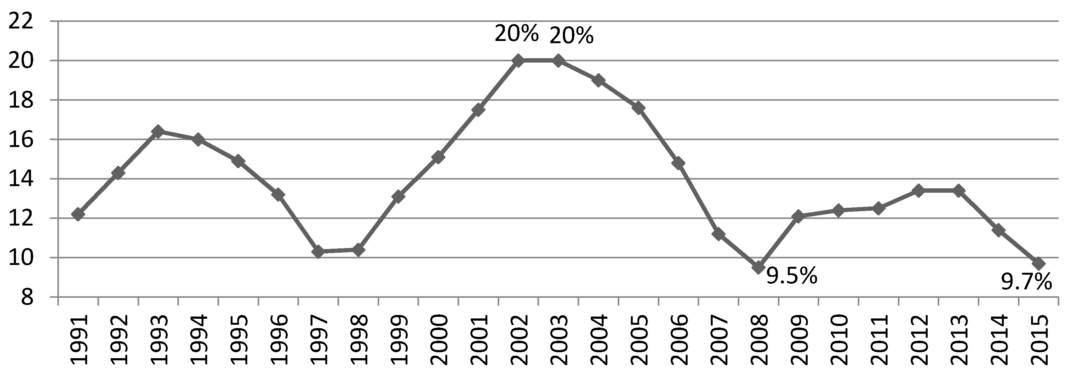
The unemployment rate in Poland has varied considerably since 1990. There have been periods when the rate has increased (1991–1993, 1999–2002, 2009–2012) and fallen (1994–1996, 2004–2008, 2014). Poland’s unemployment rate peaked at 20% in 2002 and 2003, and then fell to a low of 9.5% in 2008. In 2015, it was 9.7% (see Figure 1). Changes to the unemployment level were closely connected with the country’s economic and political situation. It was strongly affected by, for example, the expiry of obligations set forth in the privatisation agreements of the mid-1990s, which required enterprises to maintain employment at a specified level (1998–2003). Further influences were periods of economic growth (1994–1997, 2004–2008), economic crisis (after 2008), and mass migration for economic reasons connected with Poland’s accession to the European Union (after 2004).
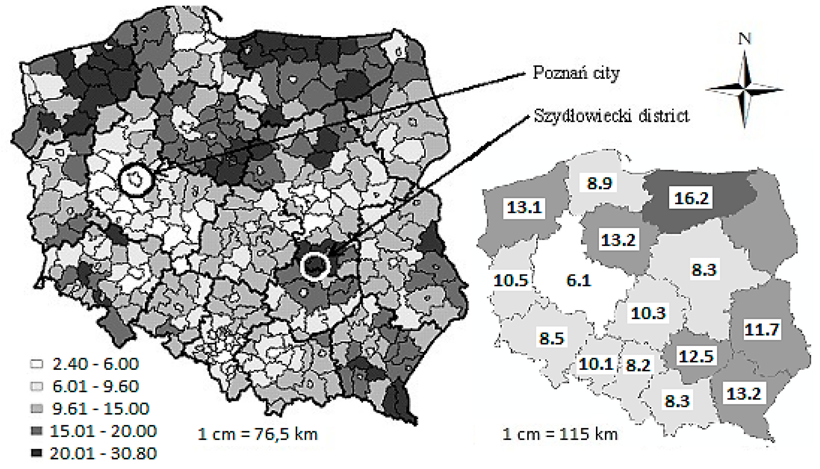
The level of unemployment in Poland has shown considerable spatial (local and regional) diversification. In 2015, the difference between districts (LAU1), characterised by the highest (the Szydlowiecki district: 30.8%) and lowest (the town of Poznan with district rights: 2.4%) unemployment levels, was as large as 28.4 percentage points. At the voivodeship level, the difference was 10.1 percentage points (between Warminsko-Mazurskie voivodeship with 16.2% and Wielkopolskie with 6.1%).
The maps presented in Figure 2 show that northern Poland has the highest unemployment rate. In contrast, the lowest values are observed in large cities: Poznan, Warsaw, Katowice, Krakow, Wroclaw and the Tricities (Gdansk, Gdynia and Sopot). Also of note, the districts located in the Mazowieckie voivodeship were among those characterised by both the highest and lowest unemployment rates, indicating the considerable diversity of economic development among spatial units located in that voivodeship.
Figure 3 shows the results of grouping districts according to unemployment rates. Unemployment rates below the national mean (9.7%) were observed in 139 districts, mainly in towns with district rights. Values fluctuated around the natural rate of unemployment (below 6%) in 38 districts (which represents 10% of all analysed units). The biggest group consists of districts where the variable ranged from 9.7% to 15%, representing 139 spatial units. Unemployment rates above 20% are observed in as many as 36 districts. In one of these, the rate exceeded 30%.
The Moran’s I statistic for the unemployment rate in 2015 was 0.47 (for the spatial weights matrix in the queen configuration, the result was statistically significant). This means that unemployment in Poland was characterised by a relatively high and positive spatial autocorrelation. Moreover, there were spatial relationships among the districts that affected the unemployment rates. Therefore, clusters of districts occurred in the geographic space, characterised by similar unemployment rates [27].
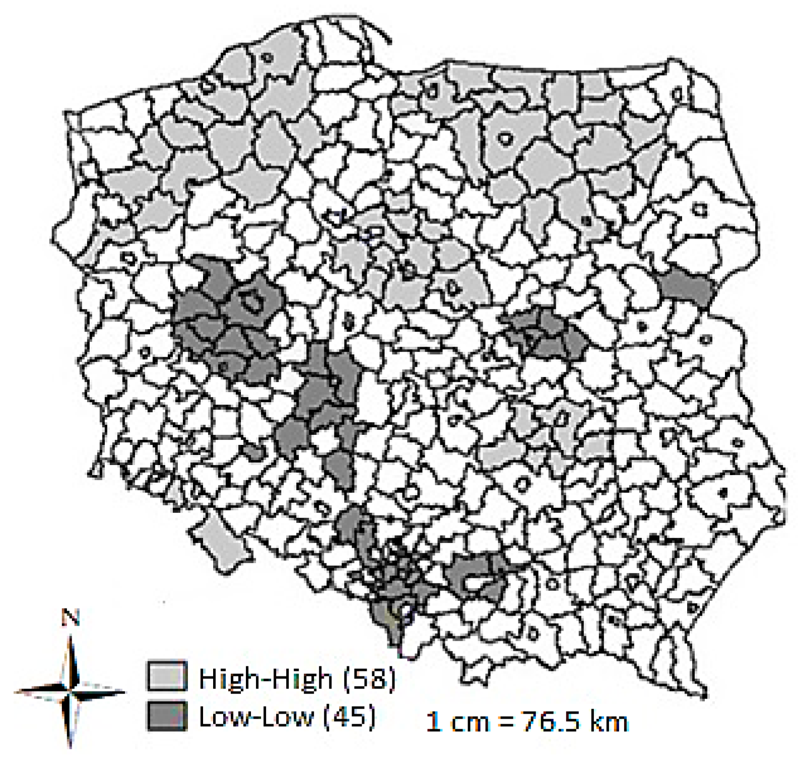
The local Moran’s statistic answers the question as to where exactly in the analysed area this phenomenon arose. In Figure 4, the areas coloured grey indicate clusters of districts characterised by similarly high unemployment rates. It is clearly visible that they are located in the northern part of the country (Zachodniopomorskie, Warminsko-Mazurskie and Kujawsko-Pomorskie voivodeships). In turn, the black areas denote clusters of spatial units with similarly low unemployment rates. They are located in cities: Poznan (Wielkopolskie voivodeship), Warsaw (Mazowieckie voivodeship) and Katowice (Slaskie voivodeship). Statistically non-significant results were obtained for the other districts (i.e., there are no spatial relationships).
Some important conclusions can be drawn from the above analysis. It shows that there were some spatial relationships among districts affecting the values of the unemployment rate in Poland. Thus, information about the relationships among the analysed spatial units ought to be considered in an econometric model describing unemployment figures in the country, for example, in the form of a spatial weights matrix.
3. Determinants of Regional Unemployment
Unemployment is a multidimensional phenomenon determined by complex factors and mechanisms. There are numerous theories offered in the literature that specify the variables which cause an increase or decrease in the unemployment rate [1]. According to Phillips [28], higher unemployment rates are accompanied by a slower rise in nominal wages, while a fall in unemployment coincides with an increase in nominal wages. The unemployment rate is also strongly related to Gross Domestic Product (on the regional level Gross Regional Product). When employment increases, the GDP rises, and thus economic growth occurs with a simultaneous fall in the unemployment rate. Okun’s law states that every 2% drop in real GDP, as compared with potential GDP, results in a rise in the unemployment rate by 1 percentage point [29]. The number of created jobs is largely dependent on the volume and type of investments. New development-oriented investments contribute to an increased demand for labour. In contrast, current investments aimed at property replacement enable existing jobs to be maintained. It should be emphasised that not all investments contribute to creating or maintaining jobs as they increase the productivity of the workforce [30]. However, greater workforce productivity enables enterprises to operate more effectively, hence, making them more competitive, and this improves the employment situation in the long run. If productivity increases significantly, it will increase the growth rate of GDP at a higher rate than productivity, which forces employers at that point to hire more workers to accommodate the expected demand. Wages will rise but if labour productivity increases at a rate faster than the increase in wages, then the rates of inflation and unemployment will decline [1].
Foundations for regional unemployment analysis are set up by the neoclassical theory, which suggests that in the long run all disparities should disappear due to labour or capital flows. Therefore, another important factor influencing the level of unemployment is migration. The most frequently mentioned motives behind migration include high unemployment rates, low wages and high costs of living. According to the world systems theory (it is a concept of social development in which the erstwhile analysed units, that is the state, economy, society, have been replaced by historical systems; the world is considered as a spatio-temporal whole), migration results from an economic imbalance between the core (i.e., developed areas-countries, regions) and peripheries (i.e., developing areas that constitute workforce reserves for the core). Since Poland’s accession to the European Union, over one million people have left the country, which resulted in a steadily declining unemployment rate from 2004 to 2008 (Figure 1). However, the unemployment rate depends not only on external migration but also, in large measure, on internal-interregional and intraregional ones. The literature suggests that propensity to migrate depends on the level of education of the employees. The highly skilled workers migrate promptly in response to a decline in regional labor demand, while the low-skilled drop out of the labor force or stay unemployed [31].
Regional studies indicate that there are some specific factors affecting regional unemployment differentials. First, conditions in a specific (regional, local) labour market that can be described by a population’s structure (e.g., the number of people of working age, number of men and women), economic activity, level of education and qualifications of local labour force, as well as the number of registered economic entities and offered jobs. Second, regional specialisation (agricultural, industrial and service) and market potential [32].
Among the factor that affect unemployment are also those of a social nature, such as social security policy (e.g., unemployment insurance benefits, family allowances). The correlation between these two factors is positive because the extensive benefits system deters job search and reduces the likelihood of migration [32].
Regrettably, not all variables significant to an analysis of unemployment were available from Polish public statistics for a LAU 1 spatial cross-section. These included, for example, inflation, GDP, level of education or regional specialisation. Because the GDP variable (describing the level of economic development) was important for this analysis, it was replaced with a local development measure which is commonly used in local analysis: districts’ budgetary income per capita. Districts’ budgetary income per capita is not as good a measure of economic development as the GDP that presents total value of goods and services produced in a country or a specific region (it aims to best capture the true monetary value of economy). Nevertheless, the amount of districts’ budgetary income depends not only on general subsidies from the state budget but also on their own revenues from local governments which include e.g., incomes from taxes (partly from personal income tax and corporate income tax) and revenues from properties, therefore it reflex wealth of regions (inhabitants) and investment activities.
The statistical database, except the unemployment rate (UR), contained the following potential determinants:
- (a)
- BE: number of business entities entered in the register per 10,000 people;
- (b)
- BI: districts’ budgetary incomes per capita in Polish zloty (PLN);
- (c)
- EM: emigration level (outflow of individuals abroad per 10,000 people);
- (d)
- FR: feminisation rate (number of women per 100 men);
- (e)
- I: capital investments in enterprises for each resident of economically productive age;
- (f)
- IM: internal migration level (outflow of individuals per 10,000 people);
- (g)
- JO: number of job offers per 10,000 people of economically productive age;
- (h)
- SA: budgetary expenditures of municipalities and towns with district rights on social assistance (division 852) per capita in PLN;
- (i)
- W: average wages in PLN.
Descriptive statistics for all variables in 2015 are presented in Table 1.
All of the explanatory variables showed positive spatial autocorrelation in 2015, it means that there are clusters of districts in geographic space characterised by similar levels of variables, e.g., high values tend to be geographic neighbours of high values [27]. The highest values of Moran’s I statistic were received for emigration, social assistance and business entities. In turn, the lowest (and statistically significant) values were obtained for capital investment, districts’ budgetary incomes, feminisation rate and job offers. Thus, there were spatial relationships (of different intensities) among districts that affected the values of those variables (Table 2).
4. Materials and Methods
The conventional approach to the empirical analyses of spatial data is to build a global model that assumes homogeneous (stationary) cross-spatial relationships between dependent and independent variables. It means that the same stimulus provokes the same response in all parts of the studied region (countries, voivodeships, districts). The regression equation can be expressed as:
where yi is the dependent variable, βk the coefficients, xki the independent variables, and εi is the error term.
However, in practice, the relationships between variables might be non-stationary and vary geographically [33]. The local linear regression, introduced to the economic context by McMillen [34], is a relatively recent modelling technique for spatial data analysis. From 1996 the technique was extended by Fotheringham, Brunsdon and Charlton [35,36,37,38] and was also renamed geographically weighted regression. Unlike global regression models, where a single coefficient is estimated for each explanatory variable, GWR enables local variations (over space) in the estimation of coefficients. Thus, the regression coefficient βk takes different values for each location. This method generates a separate regression equation for each observation, which can be expressed as follows [35]:
where yi is the dependent variable, βk the coefficients, xik the independent variables, (ui,vi) the co-ordinate location of i and εi is the error term.
The estimator for this model takes the form of:
where W(ui,vi) is the square matrix of weights relative to the position of (ui,vi) in the study area, XTW(ui,vi)X is the geographically weighted variance-covariance matrix (the estimation requires its inverse to be obtained) and Y is the vector of the values of the dependent variable [38].
The W(ui,vi) matrix contains the geographical weights in its leading diagonal and 0 in its off-diagonal elements:
Each equation is calibrated using the different weights of the observations contained in the data set. The assumption is that observations near one another have a greater influence on each other’s parameter estimates than observations farther apart, according to Tobler’s law. The weight assigned to each observation is based on a distance decay function centred on observation I [39].
GWR is a tool that is increasingly used in socioeconomic and demographic research. This is particularly true in analyses related to healthcare (e.g., incidence of diseases and access to medical services e.g., [40,41,42,43]), environmental protection (e.g., [44,45,46]), the real estate market (e.g., [47,48]), poverty (e.g., [49,50]) and migration (e.g., [51,52,53,54]). The GWR tool is also used in labour market analyses (e.g., [55,56,57,58]). However, there are few examples of studies on unemployment (see introduction) [14].
5. Results and Discussion
In order to specify local determinants of unemployment rate in Poland, geographically weighted regression, which allows to identify the variability of regression coefficients in the geographical space, was used. Several attempts were made to build the model, taking into account the different sets of explanatory variables, based on the analysis of correlation between variables, collinearity in the model, Akaike Information Criterion and coefficient of determination. Apart from the lack of data, the biggest problem in the local analysis of unemployment was the fact that some of the listed potential determinants were highly correlated with each other (it is a common problem in the analysis of regional or local unemployment [32]). The highest correlation was observed between wages and other variables, as well as feminisation rate and other variables, that is why W and FR were eliminated from further analysis in the first step. On the other hand, the lowest correlation coefficient among dependent and independent variables occurred between unemployment and number of business entities, migration and job offer, which resulted in a lack of statistical significance of BE, EM, IM and JO in the model. Eventually, the model took the following form:
where β0 is the absolute term, βk the structural parameters, (ui,vi) the longitude and latitude of districts’ centroids. Additionally, BIi is the districts’ budgetary income per capita, Ii is the capital investments in enterprises per capita in PLN and SAi is the budgetary expenditure of municipalities and towns with district rights on social assistance per capita in PLN. Finally, URi is the unemployment rate and εi is the random element.
To compare the results obtained based on the local model, the parameters of the global model were also estimated, the latter being given by the following formula:
The parameters of global model were estimated using OLS. The estimation of GWR model parameters used an estimator given by the following Formula (3). Although there are several options for the estimation methods of bandwidth in GWR models, the bi-square type kernel function was employed because it fits the best to the model. In order to select the optimum bandwidth, Corrected AIC was employed. The bandwidth where this statistic exhibit the smallest values is judged to be optimal. Table 3 presents the measures of goodness of fit used to compare both models. All measures indicate that the local model has a markedly better fit with the empirical data. The value of AIC declined from 2158.398 in global model to 2069.762 in GWR. The value of adjusted R2 improved as well. It increased from 0.497 in OLS to 0.698 (average value of adjusted local R2) in GWR. As Yu [59] notes, GWR will usually produce better fitting models than global OLS. GWR often provides a stronger result by having accounted for spatial heterogeneity of the relationship between the dependent and independent variables. Nevertheless, there is still a high unexplained variation, which must be addressed in future studies.
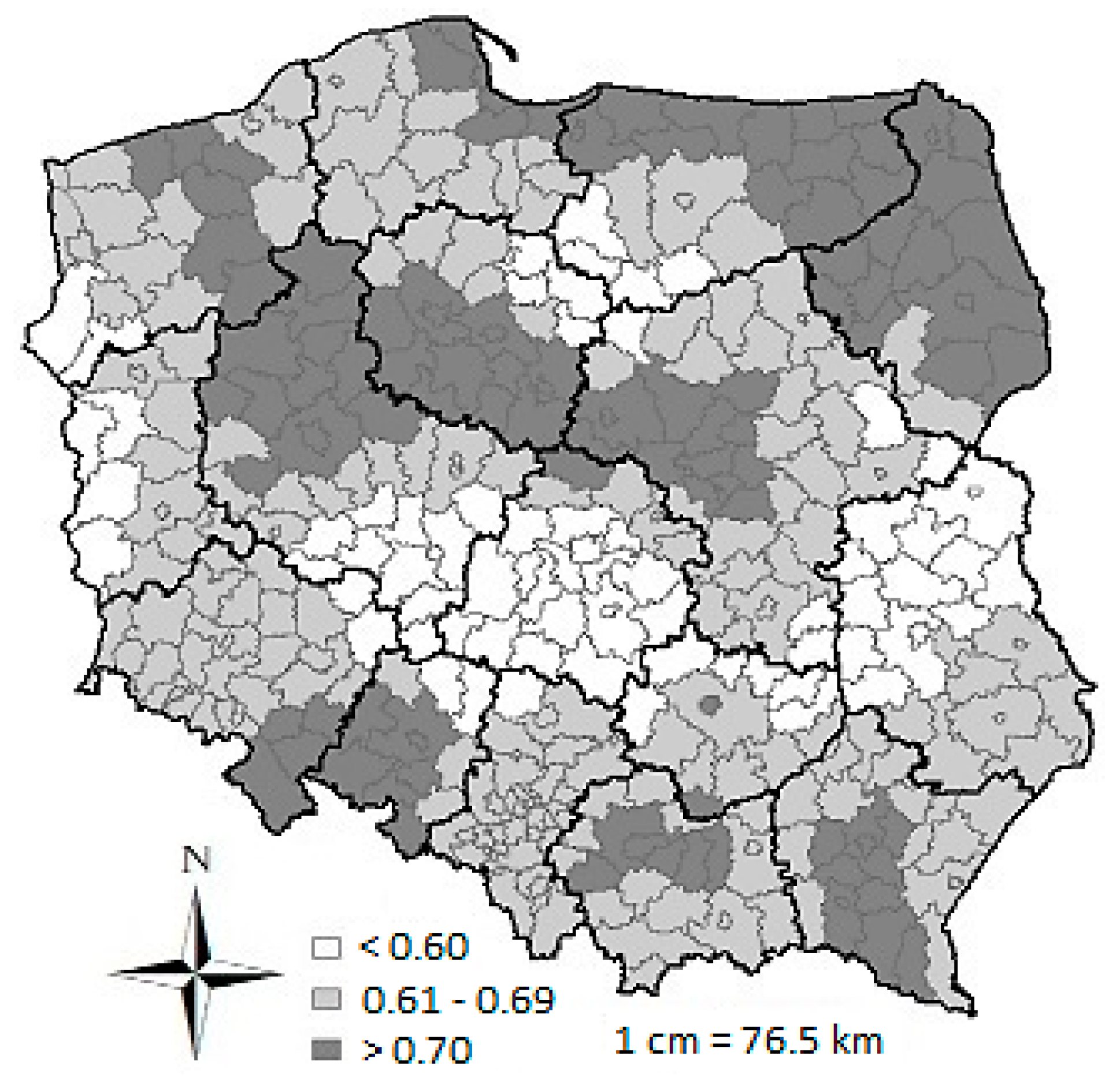
Figure 5 presents the values for the adjusted coefficients of the determination for specific GWR model locations. The map shows that the model has a poor fit with data for districts located in the central and eastern central parts of the country, particularly in the Lodzkie (e.g., the sieradzki district, adjusted R2 = 10%), Lubelskie and Wielkopolskie voivodeships. The model accurately describes the studied phenomenon in the northwestern and northern part of the country, in the districts located in the Warminsko-Mazurskie (e.g., bartoszycki district R2 = 79%), Podlaskie, Wielkopolskie, Kujawsko-Pomorskie and Mazowieckie voivodeships. The map clearly indicates that the model properly describes the studied phenomenon for a majority of spatial units.
Correlations between exogenous variables used in the model are weak (correlation coefficients do not exceed 0.4). There are therefore grounds for arguing that there is no issue of collinearity in both models, neither local nor global. In case of global model, VIF’s (Variance Inflation Factors) measure was used to test collinearity. The general rule of thumb is that VIF of 5 and above is not good for regression model because it might render other significant variables redundant [60]. Based on the results obtained (VIF do not exceed 2.3 for all variables), it can be concluded that there is no issue of collinearity in the global model. Nevertheless, collinearity may be a source of problems in GWR even when there is no collinearity in the global model [61,62]. Collinearity is potentially more of an issue in GWR because its effects can be more pronounced with the smaller spatial samples used in each local estimation and if the data are spatially heterogeneous in terms of its correlation structure, some localities may exhibit collinearity while others may not [63]. For that reason, it is difficult to make conclusion about local collinearity. Fortunately, the GWR tool in ArcMap solves this problem and simply do not present the results when there is either global or local multicollinearity in the model (in case of collinearity - global or local, the program shows an error no 040038, that stands for: “results cannot be computed because of severe model design problems” and indicates ways to deal with the problem). Based on the results of the study, it can be stated that there is no issue of collinearity in both models (global and local).
Table 4 shows the values of the regression coefficients obtained on the basis of the local and global models. In the case of the global model, one parameter was obtained for each explanatory variable. In turn, in the GWR model, the number of parameters (for each variable) equalled the number of spatial units; hence, the table shows the minimum, maximum and median values. Based on the obtained results, it can be seen that the parameters’ values fluctuated around the median of the GWR model coefficients in the global model. The minimum and maximum values, however, indicate a diversification of parameters in certain districts. It is clearly visible that the global model does not reflect the complexity of the phenomenon being studied. In contrast to the GWR model, the global model only shows averaged results and does not describe the situation in local labour markets.
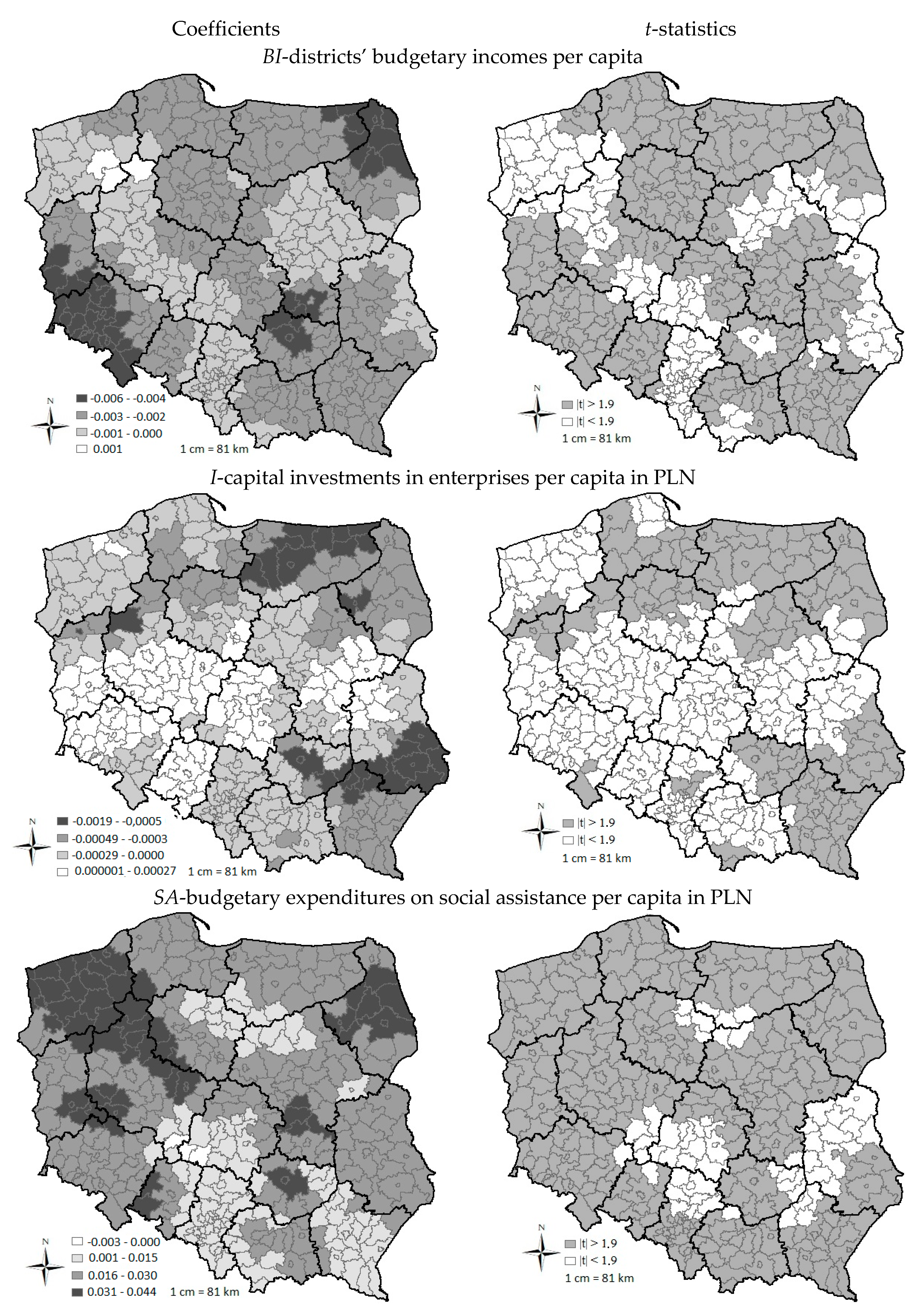
Figure 6 shows local values for the regression coefficients and the statistical significance (Student’s t statistics) of the obtained results. The maps presenting significance figures clearly show that parameters were not statistically significant for each location. This is yet further proof of the diversity of the relationships among the variables within the geographic space. The variables did not necessarily affect the unemployment rate nationwide. There were clusters of districts in the geographical space for which the parameters were statistically significant. The maps showing the parameters’ values reveal that the variables affected one another with varying intensity in the different districts. The phenomenon of clustering coefficients of similar values in the geographical space also occurred in that case. Thus, the determinants of the unemployment rate were diverse throughout the country. This diversification, however, was not consistent with the regional division (NUTS 2). The administrative boundaries of the voivodeships did not have a strong influence on this phenomenon.
A negative correlation between districts’ budgetary incomes and unemployment rate was observed in 377 districts in 2015. The strongest and most statistically significant relationship between the variables occurred in units located in the northeast in the Warminsko-Mazurskie and Podlaskie voivodeships and in the southwest, in districts located in the Dolnoslaskie voivodeship. A district’s budgetary income per capita is a measure of local development. An increased budgetary revenue indicates economic growth in a region, which results in the development of the labour market-setting up and developing enterprises, which employ more workers, thus lowering the unemployment rate. Higher revenues from administrative units’ budgets may also stimulate actions taken by the authorities to prevent unemployment (e.g., active labour market policy), including organising traineeships, training courses or social programmes.
A negative correlation was also observed between capital investments and the unemployment rate in 273 districts, mostly located in the Warminsko-Mazurskie, Podlaskie, Lubelskie and Swietokrzyskie voivodeships (the strongest relationship between those two variables was observed in the capital city of this voivodeship—town of Kielce). The situation in the labour market to a large extent depends on the level of investments made by enterprises. The number of new jobs depends on the volume and type of investments. New developmental investments have contributed to a rise in the demand for work. In contrast, current replacement investments enable already existing jobs to be maintained.
A positive correlation exists between the budgetary expenditure on social assistance of municipalities and towns with district rights and the unemployment rate in 377 districts in 2015. The strongest impact of social assistance on unemployment was observed in districts located in the following voivodeships: Zachodniopomorskie, Wielkopolskie and Podlaskie. Unemployment adversely affects social conditions and causes the loss of livelihood and qualifications, as well as increased crime and social pathology. Thus, the state can intervene in the labour market using instruments of the so-called passive labour market policy, which are usually connected with financial assistance. Excessive protectionism cannot, however, solve these problems as it may compound the decline in activity in the labour market, leading to increased unemployment. Individuals drawing unemployment benefits often do not want to take up employment as they claim that it is not profitable to do so.
Based on the results obtained by this analysis, several variables listed as potential unemployment determinants in Section 3 (e.g., migration, the number of business entities, the number of job offers and the feminisation rate) had no significant impact on the unemployment rate in districts in 2015.
6. Conclusions
This study attempted to analyse the unemployment rate in Poland in 2015 from a spatial perspective. Based on this research, it was demonstrated that the determinants of unemployment were diverse in the geographical space, as a result of political, economic and cultural differences among individual parts of the country. Poland is not a homogenous country and thus socioeconomic analyses should be performed at the local rather than national level. The specified variables did not show a significant impact on unemployment figures in all districts. Furthermore, the impact of the variables varied in intensity. It was shown that there are clusters of districts in the geographical space where variables did have a significant impact and of similar intensities. They were, however, not wholly consistent with the country’s NUTS 2 regional division.
The results of this analysis confirm the significant impact of districts’ budgetary incomes on unemployment rates in spatial units located in the northeastern and southwestern parts of the country. In turn, capital investments exerted the strongest influence on the fall in unemployment in districts located in the Warminsko-Mazurskie, Podlaskie, Lubelskie and Swietokrzyskie voivodeships. Expenditure on social assistance has an almost nationwide impact on the rise in the unemployment rate, which is very important conclusion for social policy in Poland.
GWR proved to be an extremely effective instrument of spatial data analysis. The GWR model had a considerably better fit with empirical data than the global model. It enabled the drawing of detailed conclusions concerning the local determinants of unemployment in Poland. It should, however, be emphasised that the model did not show sufficient goodness of fit to data for all analysed spatial units (e.g., for districts located in the central and central eastern parts of the country).
Due to the lack of statistical information in public statistics on the local level (LAU 1), which resulted in limited set of exploratory variables in the model, the received results should be regarded as a starting point for further analysis. As Poland is a member of the European Union, the next step should be an analysis of spatial diversification and the determinants of unemployment in European regions using GWR. Another stage in the research will be an attempt to take into account space-time data in panel GWR model, which will describe not only unemployment differentials in geographic space, but also over time.
Conflicts of Interest
The author declares no conflict of interest.
Appendix A
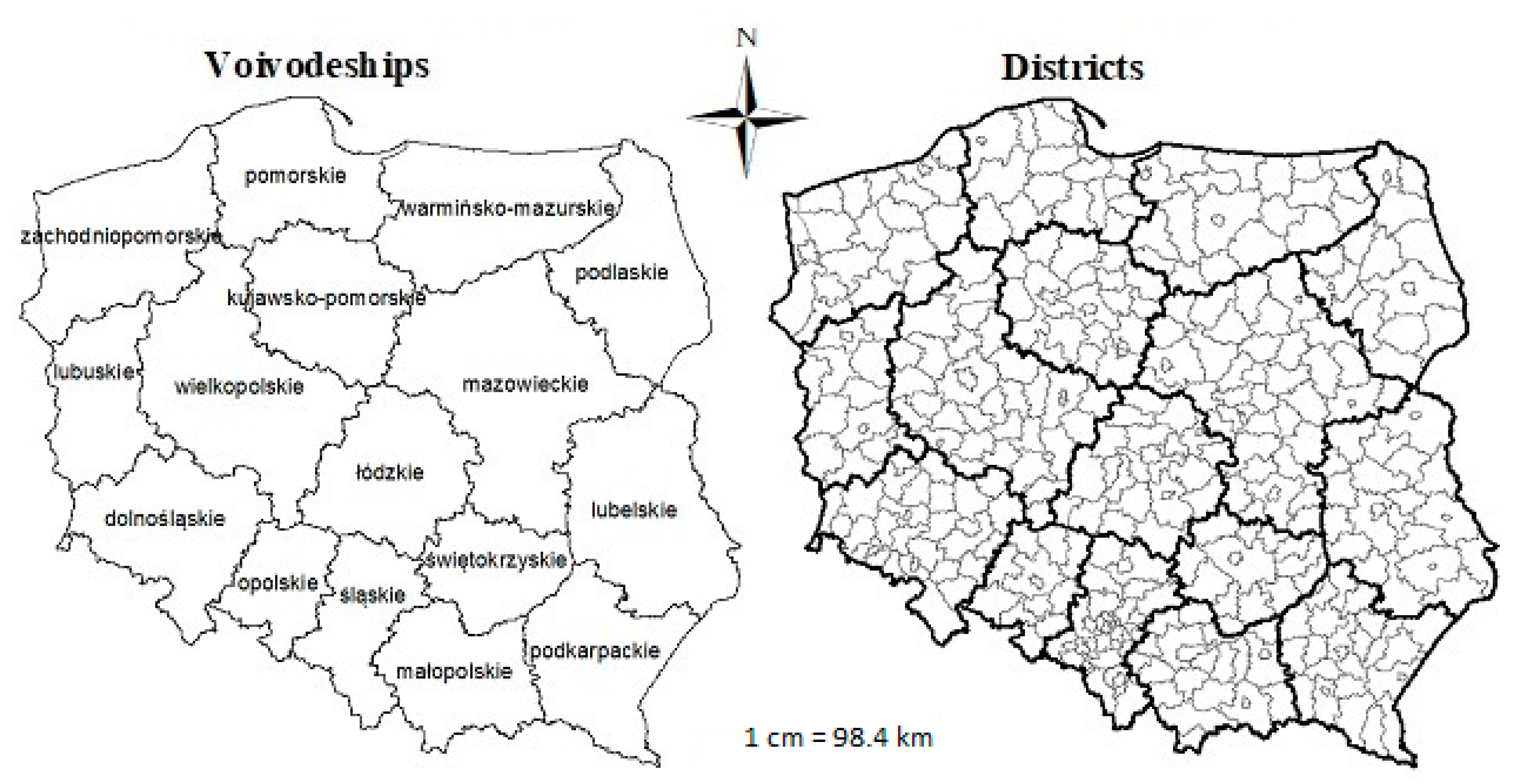
Figure A1.
Territorial division of Poland—voivodeships (NUTS 2) and districts (LAU 1). Source: Own elaboration in ArcMap 10.2.
Figure A1.
Territorial division of Poland—voivodeships (NUTS 2) and districts (LAU 1). Source: Own elaboration in ArcMap 10.2.

References
- Mouhammed, A.H. Important Theories of Unemployment and Public Policies. J. Appl. Bus. Econ. 2011, 13, 99–110. [Google Scholar]
- Beveridge, W. An Analysis of Unemployment. Economica 1936, 3, 357–386. [Google Scholar] [CrossRef]
- Clark, K.B.; Summers, L.H. Labor Market Dynamics and Unemployment: A Reconsideration. Brook. Pap. Econ. Activ. 1979, 1, 13–72. [Google Scholar] [CrossRef]
- Blank, R.; Card, D. Recent Trends in Insured and Uninsured Unemployment: Is There an Explanation? Q. J. Econ. 1991, 106, 1157–1189. [Google Scholar] [CrossRef]
- Addison, J.T.; Portugal, P. Unemployment Duration: Competing and Defective Risks. J. Hum. Resour. 2003, 38, 156–191. [Google Scholar] [CrossRef]
- Hornstein, A.; Lubik, T. The Rise in Long-Term Unemployment: Potential Causes and Implications. Econ. Q. 2015, 101, 125–149. [Google Scholar] [CrossRef]
- Lewandowska-Gwarda, K. Spatio-temporal Analysis of Unemployment Rate in Poland. Comp. Econ. Res. 2012, 15, 133–145. [Google Scholar] [CrossRef]
- Khamis, F.G. Measuring the Spatial Correlation of Unemployment in Iraq-2007. Mod. Appl. Sci. 2012, 6, 17–27. [Google Scholar] [CrossRef]
- Netrdová, P.; Nosek, V. Spatial patterns of unemployment in Central Europe: Emerging development axes beyond the Blue Banana. J. Maps 2016, 12, 701–706. [Google Scholar] [CrossRef]
- Kantar, Y.M.; Aktaş, S.G. Spatial Correlation Analysis of Unemployment Rates in Turkey. J. East. Eur. Res. Bus. Econ. 2016, 2016. [Google Scholar] [CrossRef]
- López-Bazo, E.; del Barrio, T.; Artis, M. The regional distribution of Spanish unemployment: A spatial analysis. Pap. Reg. Sci. 2002, 81, 356–389. [Google Scholar] [CrossRef]
- Rios, V. What Drives Regional Unemployment Disparities in European Regions? A Space-Time Econometric Modelling Approach. Reg. Stud. 2016, 1599–1611. [Google Scholar] [CrossRef]
- Palaskasy, T.; Psycharis, Y.; Rovolis, A.; Stoforos, C. The asymmetrical impact of the economic crisis on unemployment and welfare in Greek urban economies. J. Econ. Geogr. 2015, 15, 973–1007. [Google Scholar] [CrossRef]
- Salvati, L. Space matters: Reconstructing Local-scale Okun’s Law for Italy. Int. J. Latest Trends Financ. Econ. Sci. 2015, 5, 833–840. [Google Scholar]
- Socha, M.; Sztanderska, U. Strukturalne Podstawy Bezrobocia w Polsce; Wydawnictwo Naukowe PWN: Warszawa, Poland, 2000; ISBN 8301130067. [Google Scholar]
- Kwiatkowski, E.; Tokarski, T. Bezrobocie regionalne w Polsce w latach 1995–2005. Ekonomista 2007, 4, 439–455. [Google Scholar]
- Rogut, A. Determinanty Popytu na Pracę w Polsce w Okresie Transformacji; Wydawnictwo Uniwersytetu Łódzkiego: Łódź, Poland, 2008. [Google Scholar]
- Bartosik, K. Popytowe i podażowe uwarunkowania polskiego bezrobocia. Gospodarka Narodowa 2012, 11–12, 25–57. [Google Scholar]
- Pilc, M. Determinanty Bezrobocia w Polsce w Latach 1993–2012; CeDeWu: Warszawa, Poland, 2014; ISBN 978-83-7556-664-2. [Google Scholar]
- Boeri, T.; Scarpetta, S. Regional Mismatch and the Transition to a Market Economy. Labour Econ. 1996, 3, 233–254. [Google Scholar] [CrossRef]
- Farragina, A.M.; Pastore, F. Mind the Gap: Unemployment in the New EU Regions. J. Econ. Surv. 2008, 22, 73–113. [Google Scholar] [CrossRef]
- Munich, D.; Svejnar, J. Unemployment and Worker-Firm Matching: Theory and Evidence from East and West Europe. The World Bank, Policy Research Working Paper, No. 4810. 2009. Available online: http://hdl.handle.net/10986/4008 (accessed on 2 November 2017).
- Gorzelak, G. Poland’s Regional Policy and Disparities in the Polish Space. Studia Regionalne i Lokalne 2006, 2006, 39–74. [Google Scholar]
- Bogumił, P. Regional Disparities in Poland. ECFIN Country Focus 2009. VI. Available online: http://ec.europa.eu/economyfinance/publications/publication15180en.pdf (accessed on 20 March 2017).
- Czyż, T.; Hauke, J. Evolution of regional disparities in Poland. Quaest. Geogr. 2011, 30, 35–48. [Google Scholar] [CrossRef]
- Eurostat. Regions in the European Union. Nomenclature of Territorial Units for Statistics NUTS 2013/EU28. Eurostat Manuals and Guidelines. 2015. Available online: http://ec.europa.eu/eurostat/documents/3859598/6948381/KS-GQ-14-006-EN-N.pdf (accessed on 20 March 2017).
- Griffith, D.A. Spatial Autocorrelation and Spatial Filtering; Springer: Berlin, Germany, 2003; ISBN 978-3-540-24806-4. [Google Scholar]
- Phillips, A.W. The Relation between Unemployment and the Rate of Change on Money Wage Rates in the United Kingdom 1861–1957. Economica 1958, 25, 283–299. [Google Scholar] [CrossRef]
- Okun, A.M. Potential GNP: Its Measurement And Significance. Cowles Foundation Paper 190. 1962. Available online: https://milescorak.files.wordpress.com/2016/01/okun-potential-gnp-its-measurement-and-significance-p0190.pdf (accessed on 5 April 2017).
- Bremond, J.; Couet, J.F.; Salort, M.M. Kompendium Wiedzy o Ekonomii; Wydawnictwo Naukowe PWN: Warszawa, Poland, 2005. [Google Scholar]
- Jurajda, S.; Terrell, K. Regional unemployment and human capital in transition economies. Econ. Transit. 2009, 17, 241–274. [Google Scholar] [CrossRef]
- Elhorst, J.P. The Mystery of Regional Unemployment Differentials. Theoretical and Empirical Explanations. J. Econ. Surv. 2003, 17, 709–748. [Google Scholar] [CrossRef]
- Matthews, S.A.; Yang, T.C. Mapping the results of local statistics: Using geographically weighted regression. Demogr. Res. 2016, 26, 151–166. [Google Scholar] [CrossRef] [PubMed]
- McMillen, D. One hundred fifty years of land values in Chicago: A nonparametric approach. J. Urban Econ. 1996, 40, 100–124. [Google Scholar] [CrossRef]
- Brunsdon, C.; Fotheringham, S.; Charlton, M. Geographically Weighted Regression: A Method for Exploring Spatial Nonstationarity. Geogr. Anal. 1996, 28, 281–298. [Google Scholar] [CrossRef]
- Fotheringham, A.S.; Charlton, M.; Brunsdon, C. Measuring Spatial Variations in Relationships with Geographically Weighted Regression. In Recent Developments in Spatial Analysis; Fischer, M., Getis, A., Eds.; Springer: London, UK, 1997; pp. 60–82. ISBN 978-3-662-03499-6. [Google Scholar]
- Fotheringham, A.S.; Brunsdon, C.; Charlton, M. Geographically Weighted Regression: The Analysis of Spatially Varying Relationships. Geogr. Anal. 2003, 28, 281–298. [Google Scholar] [CrossRef]
- Charlton, M.; Fotheringham, A.S. Geographically Weighted Regression. Available online: http://gwr.nuim.ie/downloads/GWR_WhitePaper.pdf (accessed on 10 April 2017).
- Mennis, J. Mapping the Results of Geographically Weighted Regression. Cartogr. J. 2006, 43, 171–179. [Google Scholar] [CrossRef]
- Nakaya, T.; Fotheringham, A.S.; Brunsdon, C.; Charlton, M. Geographically weighted Poisson regression for disease association mapping. Stat. Med. 2005, 24, 2695–2717. [Google Scholar] [CrossRef] [PubMed]
- Young, L.J.; Gotway, C.A. Using geostatistical methods in the analysis of public health data: The final frontier? Quant. Geol. Geostat. 2010, 16, 89–98. [Google Scholar] [CrossRef]
- Comber, A.J.; Brunsdon, C.; Radburn, R. A spatial analysis of variations in health access: Linking geography, socio-economic status and access perceptions. Int. J. Health Geogr. 2011, 10, 44–55. [Google Scholar] [CrossRef] [PubMed]
- Christman, Z.; Pruchno, R.; Cromley, E.; Wilson-Genderson, M.; Mir, I. Spatial Analysis of Body Mass Index and Neighborhood Factors in Community-Dwelling Older Men and Women. Int. J. Aging Hum. Dev. 2016, 83, 3–25. [Google Scholar] [CrossRef] [PubMed]
- Foody, G.M. Geographical weighting as a further refinement to regression modelling: An example focused on the NDVI-rainfall relationship. Remote Sens. Environ. 2003, 88, 283–293. [Google Scholar] [CrossRef]
- Gilbert, A.; Chakraborty, J. Using geographically weighted regression for environmental justice analysis: Cumulative cancer risks from air toxics in Florida. Soc. Sci. Res. 2011, 40, 273–286. [Google Scholar] [CrossRef]
- Fu, J.; Jiang, D.; Lin, G.; Liu, K.; Wang, Q. An ecological analysis of PM2.5 concentrations and lung cancer mortality rates in China. BMJ Open 2015, 5, e009452. [Google Scholar] [CrossRef] [PubMed]
- Yu, D.-L.; Wei, Y.; Wu, C. Modelling spatial dimensions of housing prices in Milwaukee, WI. Environ. Plan. B Plan. Des. 2007, 34, 1085–1102. [Google Scholar] [CrossRef]
- Cellmer, R. The Use of the Geographically Weighted Regression for the Real Estate Market Analysis. Folia Oecon. Stetin. 2013, 11, 19–32. [Google Scholar] [CrossRef]
- Benson, T.; Chamberlin, J.; Rhinehart, I. An investigation of the spatial determinants of the local prevalence of poverty in rural Malawi. Food Policy 2005, 30, 532–550. [Google Scholar] [CrossRef]
- Partridge, M.D.; Rickman, D.S. The Geography of American Poverty: Is There a Need for Place-Based Policies? Growth Chang. 2009, 40, 169–174. [Google Scholar] [CrossRef]
- Byrne, G.; Pezić, A. Modelling Internal Migration Drivers with Geographically Weighted Regression. In Proceedings of the 12th Biennial Conference of the Australian Population Association, Canberra, Australia, 15–17 September 2004; pp. 1–9. Available online: http://arrow.latrobe.edu.au:8080/vital/access/manager/Repository/latrobe:613 (accessed on 15 April 2017).
- Jensen, T.; Deller, S. Spatial Modelling of the Migration of Older People with a Focus on Amenities. Rev. Reg. Stud. 2007, 37, 303–343. [Google Scholar]
- Jivraj, S.; Brown, M.; Finney, N. Modelling Spatial Variation in the Determinants of Neighbourhood Family Migration in England with Geographically Weighted Regression. Appl. Spat. Anal. Policy 2013, 6, 285–304. [Google Scholar] [CrossRef]
- Lewandowska-Gwarda, K. Spatial Analysis of Foreign Migration in Poland Using Geographically Weighted Regression. Comp. Econ. Res. 2014, 17, 137–154. [Google Scholar] [CrossRef]
- Dell’Aringa, C.; Lucifora, C.; Origo, F. Public Sector Pay and Regional Competitiveness: A First Look at Regional Public-Private Wage Differentials in Italy. Manch. Sch. 2007, 75, 445–478. [Google Scholar] [CrossRef]
- Li, T.; Corcoran, J.; Pullar, D.; Robson, A.; Stimson, R. A Geographically Weighted Regression Method to Spatially Disaggregate Regional Employment Forecasts for South East Queensland. Appl. Spat. Anal. Policy 2009, 2, 147–175. [Google Scholar] [CrossRef]
- Patuelli, R.; Schanne, N.; Griffith, D.A.; Nijkamp, P. Persistence of Regional Unemployment: Application of a Spatial Filtering Approach to Local Labor Markets in Germany. J. Reg. Sci. 2012, 52, 300–323. [Google Scholar] [CrossRef]
- Pijnenburg, K. Self-Employment and Economic Performance. A Geographically Weighted Regression Approach for European Regions. Available online: https://www.diw.de/documents/publikationen/73/diw_01.c.416595.de/dp1272.pdf (accessed on 10 May 2017).
- Yu, D.-L. Spatially varying development mechanisms in the Greater Beijing area: A geographically weighted regression investigation. Ann. Reg. Sci. 2006, 40, 173–190. [Google Scholar] [CrossRef]
- Akinwande, M.O.; Dikko, H.G.; Samson, A. Variance Inflation Factor: As a Condition for the Inclusion of Suppressor Variable(s) in Regression Analysis. Open J. Stat. 2015, 5, 754–767. [Google Scholar] [CrossRef]
- Wheeler, D.; Tiefelsdorf, M. Multicollinearity and Correlation among Regression Coeffcients in Geographically Weighted Regression. J. Geogr. Syst. 2005, 7, 161–187. [Google Scholar] [CrossRef]
- Wheeler, D. Diagnostic Tools and a Remedial Method for Collinearity in Geographically Weighted Regression. Environ. Plan. A 2007, 39, 2464–2481. [Google Scholar] [CrossRef]
- Gollini, I.; Lu, B.; Charlton, M.; Brunsdon, C.; Harris, P. GWmodel: An R Package for Exploring Spatial Heterogeneity Using Geographically Weighted Models. J. Stat. Softw. 2015, 63. [Google Scholar] [CrossRef]
Figure 1.
Unemployment rate in Poland (1990–2015). Source: Own elaboration.

Figure 2.
Unemployment rates in Poland by district (LAU 1) and voivodeship (NUTS 2) in 2015. Source: Own elaboration in ArcMap 10.2.
Figure 2.
Unemployment rates in Poland by district (LAU 1) and voivodeship (NUTS 2) in 2015. Source: Own elaboration in ArcMap 10.2.

Figure 3.
Districts grouped according to unemployment rate in 2015. Source: Own elaboration.

Figure 4.
Local Moran’s statistic for unemployment rates in Poland in 2015. Source: Own elaboration in GeoDa.
Figure 4.
Local Moran’s statistic for unemployment rates in Poland in 2015. Source: Own elaboration in GeoDa.

Figure 5.
Local adjusted R2 in the Geographically Weighted Regression (GWR) model. Source: Own elaboration in ArcMap 10.2.
Figure 5.
Local adjusted R2 in the Geographically Weighted Regression (GWR) model. Source: Own elaboration in ArcMap 10.2.

Figure 6.
Local values of coefficients and t-statistics in the GWR model. Source: Own elaboration in ArcMap 10.2.
Figure 6.
Local values of coefficients and t-statistics in the GWR model. Source: Own elaboration in ArcMap 10.2.


Table 1.
Descriptive statistics for variables in 2015.
| Variable | Minimum | Mean | Median | Maximum | Standard Deviation |
|---|---|---|---|---|---|
| BE | 46.95 | 91.82 | 87.65 | 230.55 | 27.36 |
| BI | 2745.80 | 3680.00 | 3408.50 | 8228.20 | 805.58 |
| EM | 0.00 | 7.14 | 5.33 | 42.87 | 6.12 |
| FR | 95.65 | 104.68 | 103.80 | 119.76 | 3.83 |
| I | 396.48 | 5446.30 | 4008.90 | 51,570.00 | 5709.60 |
| IM | 0.00 | 5.82 | 3.23 | 122.60 | 27.36 |
| JO | 0.04 | 15.82 | 6.50 | 294.17 | 29.71 |
| SA | 294.97 | 571.23 | 554.89 | 1017.90 | 130.71 |
| UR | 2.40 | 12.27 | 11.65 | 30.80 | 5.27 |
| W | 2544.20 | 3532.30 | 3414.30 | 6955.90 | 493.35 |
Number of observation = 380; Source: Own elaboration.
Table 2.
Values of Moran’s I statistics for potential determinants of unemployment in Poland in 2015.
Table 2.
Values of Moran’s I statistics for potential determinants of unemployment in Poland in 2015.
| Variable | Moran’s Statistic I |
|---|---|
| BE | 0.44 * |
| BI | 0.14 * |
| EM | 0.58 * |
| FR | 0.17 * |
| I | 0.07 * |
| IM | 0.30 * |
| JO | 0.18 * |
| SA | 0.49 * |
| W | 0.21 * |
* statistically significant; Source: Own elaboration.
Table 3.
Diagnostic statistics for local and global models.
| Local Model GWR | Global Model | |
|---|---|---|
| Coefficient determination R2 | 0.776 | 0.501 |
| Adjusted R2 | 0.698 | 0.497 |
| Akaike Information Criterion | 2069.762 | 2158.398 |
Source: Own elaboration.
Table 4.
Regression coefficients in local and global models.
| Variable | Local Model GWR | Global Model | ||
|---|---|---|---|---|
| Minimum | Median | Maximum | ||
| Constant | −14.857 | 10.666 | 24.519 | 9.93 |
| BIi | −0.006 | −0.003 | 0.0009 | −0.003 |
| Ii | −0.002 | −0.0001 | 0.0003 | −0.0001 |
| SAi | −0.003 | 0.021 | 0.044 | 0.022 |
Source: Own elaboration.
© 2018 by the author. Licensee MDPI, Basel, Switzerland. This article is an open access article distributed under the terms and conditions of the Creative Commons Attribution (CC BY) license (http://creativecommons.org/licenses/by/4.0/).
Share and Cite
MDPI and ACS Style
Lewandowska-Gwarda, K. Geographically Weighted Regression in the Analysis of Unemployment in Poland. ISPRS Int. J. Geo-Inf. 2018, 7, 17. https://0-doi-org.brum.beds.ac.uk/10.3390/ijgi7010017
AMA Style
Lewandowska-Gwarda K. Geographically Weighted Regression in the Analysis of Unemployment in Poland. ISPRS International Journal of Geo-Information. 2018; 7(1):17. https://0-doi-org.brum.beds.ac.uk/10.3390/ijgi7010017
Chicago/Turabian StyleLewandowska-Gwarda, Karolina. 2018. "Geographically Weighted Regression in the Analysis of Unemployment in Poland" ISPRS International Journal of Geo-Information 7, no. 1: 17. https://0-doi-org.brum.beds.ac.uk/10.3390/ijgi7010017
Note that from the first issue of 2016, this journal uses article numbers instead of page numbers. See further details here.