Graph-Optimization-Based ZUPT/UWB Fusion Algorithm


School of Computer Science and Technology, China University of Mining and Technology, Xuzhou 221116, China
*
Author to whom correspondence should be addressed.
ISPRS Int. J. Geo-Inf. 2018, 7(1), 18; https://0-doi-org.brum.beds.ac.uk/10.3390/ijgi7010018
Submission received: 3 October 2017
/
Revised: 21 December 2017
/
Accepted: 8 January 2018
/
Published: 10 January 2018
Abstract
:The potential of multi-sensor fusion for indoor positioning has attracted substantial attention. A ZUPT/UWB data fusion algorithm based on graph optimization is proposed in this paper and is compared with the traditional fusion algorithms, which are based on particle filtering. With a series of observations, the proposed algorithm can achieve higher precision with acceptable computational complexity. Two methods for dynamically determining the confidence level are also presented. The first method can reduce the confidence level of ZUPT at corners, and the second method can determine the lower bound on the UWB sensor’s confidence level through the UWB optimized residual. Experimental results demonstrate the ability of the proposed method to achieve a positioning accuracy of 0.4 m, which is better than the 0.7 m achieved by the particle-filtering-based fusion method.
1. Background Description
Indoor positioning has made considerable progress in the context of the popularity of location-based services, but progress concerning positioning accuracy has come to a standstill due to limited hardware performance and costs. Recent years have witnessed a growing need for high-accuracy indoor positioning techniques, underscoring the necessity for developing a high-accuracy low-cost indoor positioning system. As a result, multi-sensor data fusion methods have been brought to the fore [1]. Algorithms of this type include the IMU (Inertial Measurement Unit) and wireless positioning techniques such as UWB (Ultra-wideband) [2,3], WiFi [4,5], and Bluetooth [6]. An accurate location can be obtained in the short term through integrating the IMU measurements, but this approach belongs to an incremental positioning system that produces cumulative error. Wireless positioning techniques perform poorly for single-point positioning, and their positioning accuracy and stability fall short of expectations, especially in complicated scenarios. However, the wireless positioning techniques are free from cumulative error. By combining the two types of sensors, it is possible to overcome their disadvantages and produce exceptionally high positioning accuracy.
The general multi-sensor fusion methods are largely dependent on the Bayes filtering framework. Typical examples include EKF (Extended Kalman Filter) [7,8] and PF (Particle Filter) [9,10,11]. The basic idea behind these methods is to assume that the current status is correlated only with the previous status and the current observation. Although the information from previous moments is still incorporated into the estimate of the current status, these methods naively assume that the current status is related only to the previous status [12,13,14]. As a result, the sequence of previous statuses and the information contained in their corresponding observations must be compressed, thereby leading to underuse of information. To address this problem, a graphical-description-based optimization method was proposed in the visual positioning field; this method is also known as graph optimization.
The largest difference between the graph optimization method and the Bayes filtering method is that the former makes no Markov assumption and directly maintains the previous statuses [15]. The solution obtained with the graph optimization method is the optimal result under a series of constraints. Although the graph optimization method determines its optimal solution through linear iteration near the operating point while solving the Jacobian matrix, its solution is more accurate than those of EKF, IEKF (Iterated Extended-Kalman Filter) and PF, which easily fall into a local minimum of the real probability distribution function due to the absence of long-term memory during the state estimation process. Because the observation model in the ZUPT/UWB fusion algorithm is far from being a linear model, the probability distribution function is complex and difficult to reduce to a simple function such as the Gaussian distribution function in EKF or a non-linear distribution function simulated by particles in PF. Given that premise, even EKF and PF can easily find the global minimum of the simplified distribution function, and there is a considerable difference between this solution and the global minimum of the real probability distribution function.
Graph-optimization-based back-end optimization plays a crucial role in many of the state-of-art SLAM algorithms that have been proposed in recent years. The Direct Sparse Odometry method, which was proposed by J. Engel et al. [16,17], was characterized by considerable accuracy and robustness. The graph optimization scheme was successfully applied to feature-based visual SLAM [18] and laser SLAM [19]. By fully exploiting the correlation between previous statuses, these SLAM algorithms achieved remarkable performance gains in terms of positioning accuracy over the traditional SLAM algorithms, which are based on EKF or PF. However, they are rarely used for multi-sensor data fusion in the IMU-based positioning framework.
IMU and UWB are combined in this paper through graph optimization. The paper is organized as follows. Section 2 covers the description of the algorithm. We first discuss the basic UWB positioning method in Section 2.1 and briefly introduce the particle-filtering-based IMU/UWB fusion algorithm in Section 2.2. The basic theory of graph optimization is discussed in Section 2.3.1. In Section 2.3.2, we present the graph-optimization-based IMU/UWB fusion algorithm. In Section Method for Dynamically Determining the ZUPT Confidence Level and Section Method for Dynamically Determining the UWB Confidence Level, we propose two methods for dynamically determining the confidence level of the ZUPT (Zero-velocity Update) output data and the UWB output data, respectively. Section 3 covers the experiments and results. We compare the proposed algorithm with other algorithms and prove the validity and effectiveness of the two confidence-level calculation methods. Finally, we present our conclusions in Section 4.
2. Algorithm Description
2.1. UWB Positioning Based on a Single Measurement
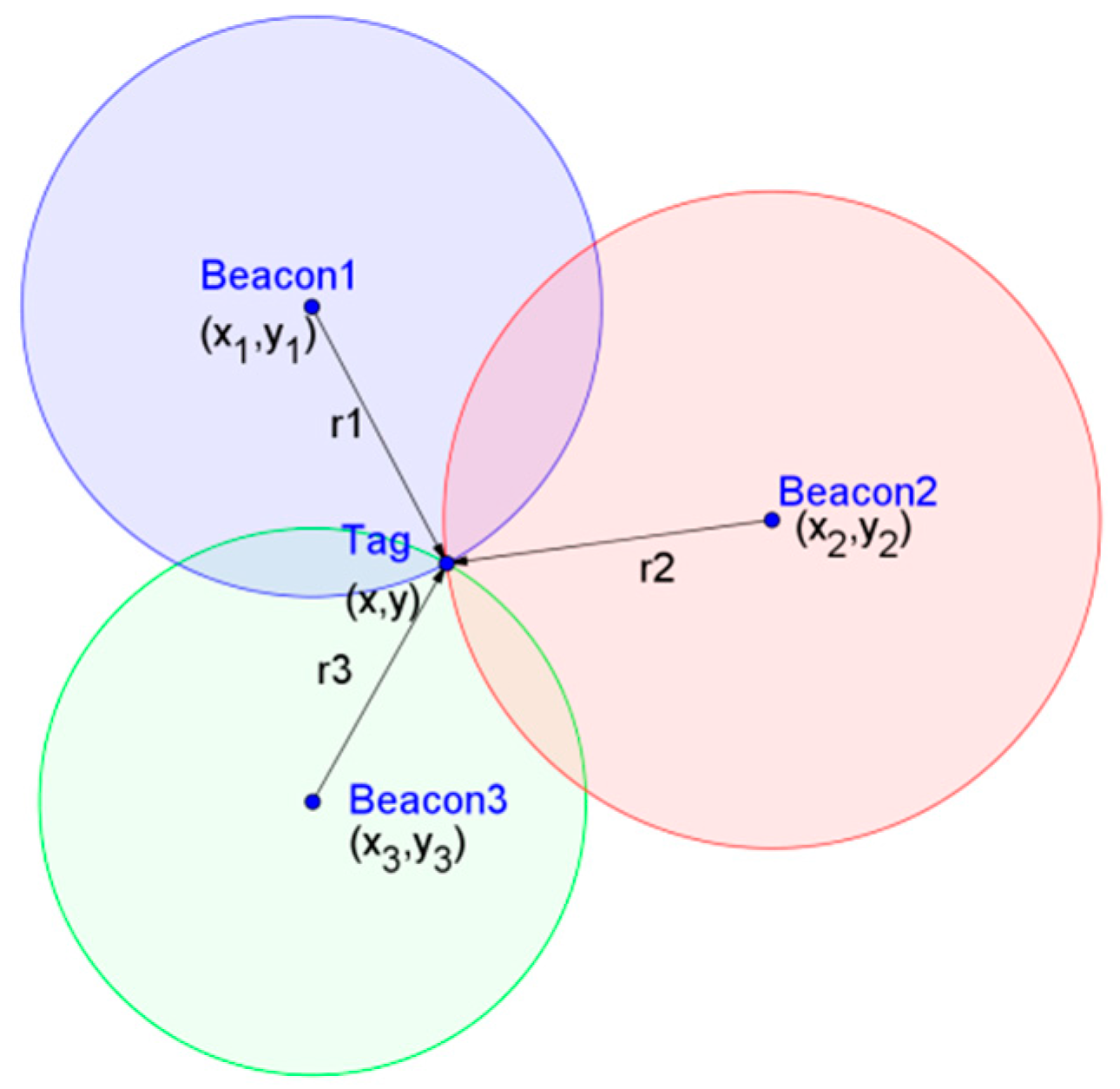
The UWB sensor positioning algorithm is largely dependent on the TOA (Time of Arrival) and TDOA (Time difference of Arrival) methods [20]. Let denote the ith UWB station in the plane positioning scenario and denote its coordinates. Let Tag denote the UWB tag used for positioning and its coordinates. The measurement collected by the UWB sensor based on TOA represents the distance between Tag and Beacon. Let denote the actual distance between Tag and , and denote the measured distance. As shown in Figure 1, ideally, . Note that a point can be identified uniquely from the intersection of the three circles, and the coordinates of this point denote the Tag location obtained from the current observation. We have two approaches for determining this point: We can adopt the trilateration method, in which a location is calculated directly using the coordinates of three points, or we can define the constrained relationship between Tag and Beacon, define an error function, and then determine the coordinates of Tag by minimizing the error function. The latter approach is more general because more beacons are available under important scenarios for improving the positioning accuracy. A feasible error function is
where denotes the absolute value function. The coordinates can be determined by minimizing .
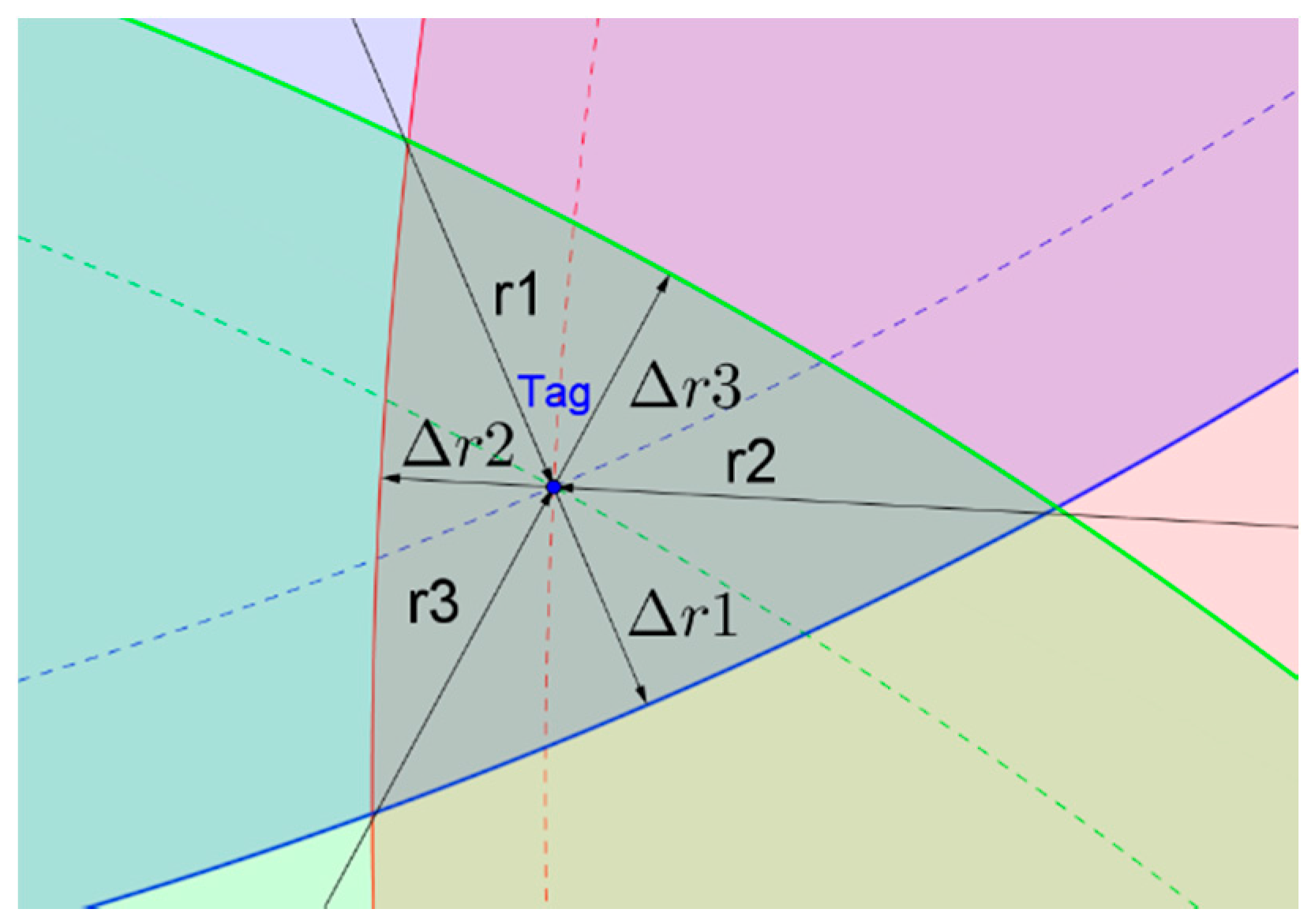
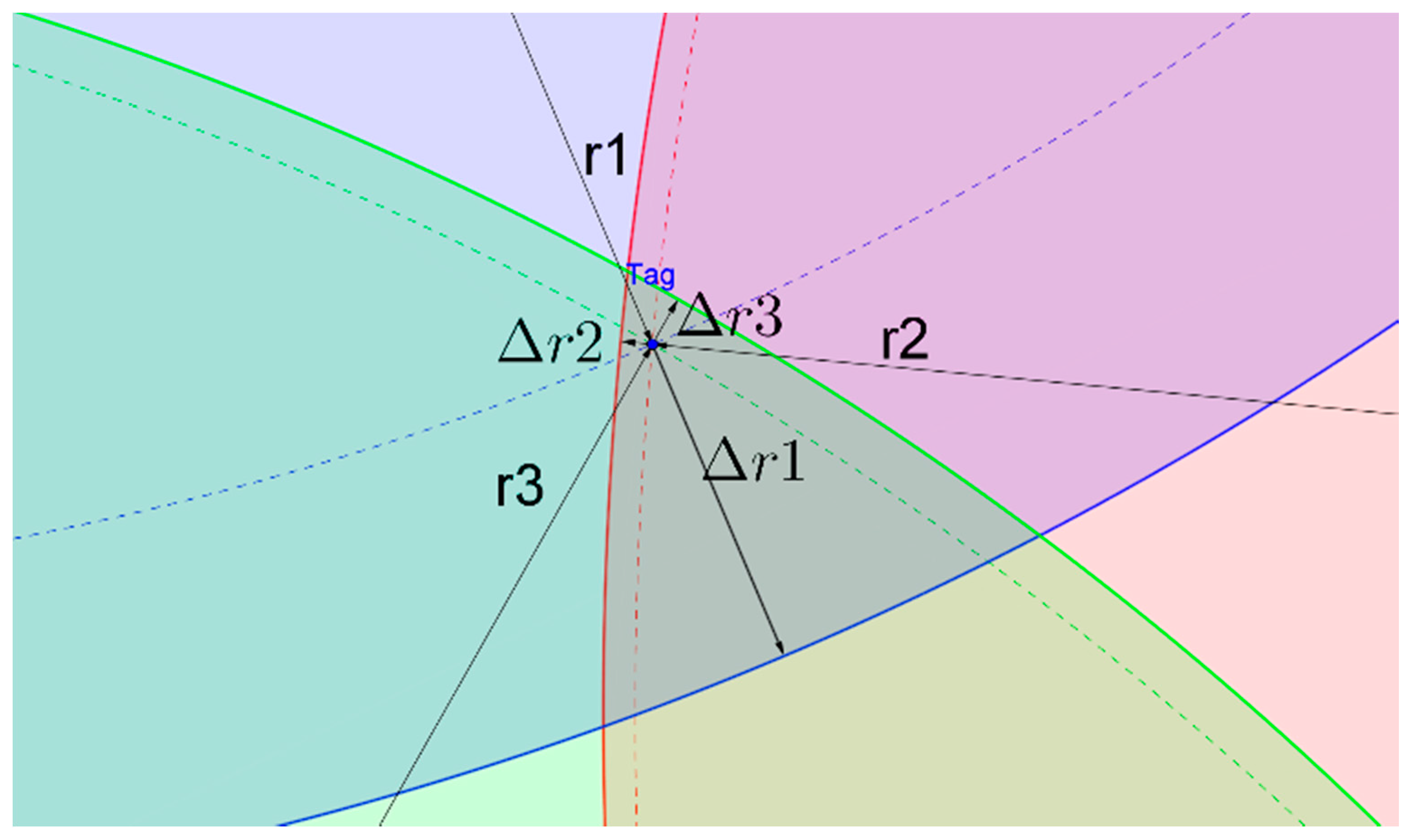
This method is called UWB-optimize in this paper, and it is mainly used to indirectly represent the quality of UWB observations. The minimal value of is 0 in the ideal scenario of Figure 1. However, there are measurement errors in real-world applications from system noise and NLOS (Non Line of Sight) environments [21,22]. To describe this situation, we still let denote the actual distance and let denote the deviation of . To measure , we use . Assuming that the beacon measurement corresponds to a circle, Figure 2 shows the overlapped region of three circles that correspond to three beacons near Tag. When the measurements contain errors, the three circles intersect in a pairwise manner rather than at one point. In this case, the estimated coordinate of Tag can still be determined by minimizing . is positively correlated to . That is, increases with . This property will be used afterwards to dynamically obtain the confidence level of the UWB observations.
Single-measurement-based UWB positioning systems are easy to implement and incur only small computational loads. Because only one measurement is used for positioning, when the quality of that measurement is poor, the accuracy of this method will be seriously affected. Moreover, UWB sensors are expensive and their sensing error is significant in NLOS environments, which highlights the need for fusion with other sensors in real-world applications. Hence, a more general approach is to improve the positioning accuracy and robustness through multi-sensor fusion with the Bayes filter.
2.2. Particle-Filtering-Based UWB and UWB/INS Fusion Algorithm
The Bayes filter is the most commonly used method for state estimation. In the particle filter, many particles are used to estimate the state’s a posteriori distribution. Compared with the EKF method, which addresses non-linear problems through linear approximation, the particle filter is more effective in terms of UWB positioning. The reason is that the observation model of the UWB sensor is highly non-linear and linearizing this model will cause serious error. Therefore, it is of great significance to study the particle-filter-based UWB positioning method and the UWB/INS fusion-based positioning method. In this paper, we describe the pure UWB algorithm based on a particle filter (UWB-PF) and the UWB/INS fusion algorithm based on particle filter (Fusing), which are used for comparisons with the proposed method based on graph optimization.
Assume that there are N known beacons in total and that the coordinates of these beacons are known in advance; we denote them as . Let and denote the set of particles and their weights at t − 1, respectively, where denotes the status of the ith particle at t − 1, and denotes the weight of the ith particle at t − 1. Note that these quantities are known at t. Assume that the system status of the current moment is related only to the status of the previous moment and the input of the current moment. The system status can be updated by collecting samples, updating the weights using the observation model and then calculating the positioning result. The Resample step should be added to inhibit particle attenuation. Note that when we determine the position by computing the weighted average of the particle statuses, the weight is the normalized value of all weights.
The sampling process of particle filtering is responsible for obtaining the particle’s a priori distribution at t by sampling the particles at t − 1 through the output of the IMU. The particle updating process follows the distribution , where denotes the system’s status transition equation. Due to loose coupling between IMU and UWB, we define the rates of change of the speed and angle in terms of the relationship between the two sensors to simplify the calculations and the model. Under this strategy, the particle’s status includes its coordinates, line speed and angle, and its status vector can be written as . Let denote the input of IMU to the particle filter, which represents the variations in speed and moving direction from the previous moment to the current moment. (In UWB-PF, the variations are zero.) Obviously, this form of status transition equation is not linear, and each quantity can be updated as follows:
These equations can be used to approximate the a priori distribution at t. In what follows, we need to determine the particle’s a posteriori distribution by updating the particle weights using the observations. Each particle weight is in direct proportion to the posterior probability, and the posterior probability can be obtained by computing the product of the prior probability and the likelihood probability. It can be updated as follows:
where denotes the distance between each station and tag, and denotes the distance between the jth station and the current tag at t. We can normalize all the weights. Because the weight represents the posterior probability of the corresponding particle’s status, the scalar form of the likelihood function can be written as
According to the UWB observation model, the likelihood function can be rewritten as
where denotes the standard deviation of the UWB observation, g denotes the error model of the UWB sensor, and denotes the distance between the i-th particle’s current status and the j-th station. Because the UWB sensors are not in same plane, the observation values of UWB should be projected into the x-o-y plane, which is easy to implement because the differences in altitude between the UWB stations and the tags are measurable in real applications. It is assumed in this paper that the sensor’s measurements follow the normal distribution with a mean equal to the actual value and a standard deviation of .
The particle filter describes the system status using many particles. By jointly considering the outputs of two types of sensors, it achieves a remarkable improvement in positioning accuracy, even when the UWB observations are highly erroneous. In contrast, the Bayes filter considers only the relationship between the current status and previous status. The path obtained using the Bayes filter will deviate greatly from the ground truth when errors occur at consecutive moments.
2.3. Graph-Fusing Model
2.3.1. Fundamentals of Graph Optimization Theory
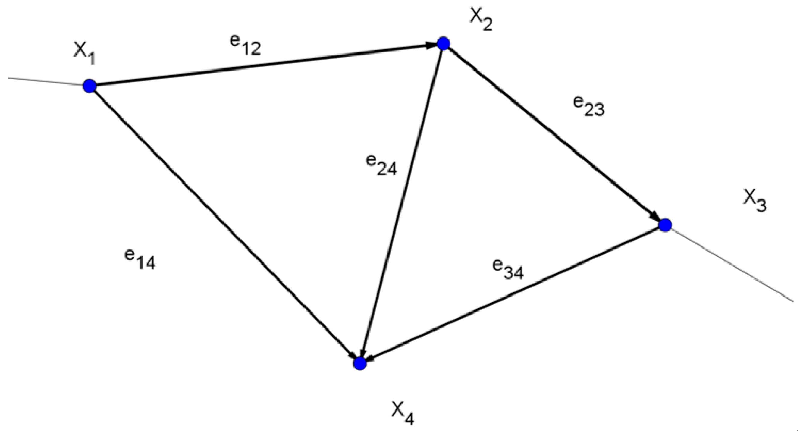
The graph optimization technique is designed to intuitively describe the complex relationship between statuses and convert it into a cost function for optimization purposes. Generally, the system status is formulated as a vertex of a graph in graph optimization theory, and the relationship between statuses is represented by an edge of a directed graph [23]. Figure 3 shows a typical example of the graph optimization structure, where each blue round spot represents a status during graph optimization and a vector between vertices represents the relationship between statuses. Specifically, denotes the difference between the observation and the relationship between and . Note that is zero when the relationship between and is completely consistent with . The larger the deviation from the observation is, the larger the value of is. We can construct a cost function and then obtain an estimate of each status by minimizing this function. Consider the example in Figure 3. Its cost function is defined as follows:
where denotes all the statuses and denotes the information matrix of , which represents the confidence level of the current status. Obtaining the optimal estimate of the statuses involves minimizing .
The quantity is related to , , and . For the sake of simplifying notation, the cost function is defined as
is omitted, as it remains unchanged during optimization. Thus, the cost function can be written as
and further rewritten as
The general methods for obtaining the optimal estimate of a status are the Gauss-Newton and LM algorithms. Both involve linearizing the cost function at the current guess status (denoted by ). That is, they approach the cost function through the first-order Taylor expansion of , and then obtain by iteratively computing the local extreme value. In fact, the EKF algorithm is an incremental algorithm for solving the same cost function. Because the cost function for each part is linearized only once in the whole process, the computational complexity of EKF is lower than that of the Gauss-Newton or LM algorithms. Let denote the status increment. The cost function is represented by and the current guess, , can be written as follows:
The quadratic form of the cost function of can facilitate the calculation of the local extreme value. Hence, in the equation needs to be expressed as a linear function of . Through the use of its first-order Taylor expansion, it can be written as
where .
Substituting the Taylor expansion into the cost function, we have
Regarding its quadric form, we can compute its extreme value by setting its partial derivative to 0:
We then have
After simplifying the above equation while taking the matrix form into account, it is shown that the solution to the equation for satisfies the following condition:
where b is a constant term and denotes the coefficient of .
The Levenberg-Marquardt algorithm provides an effective and robust approach for solving this problem; in many cases, it finds a solution even if it starts very far from the final minimum [24]. By introducing a damping coefficient into this formula to control the convergence rate, we obtain the following linear expression:
where denotes the damping coefficient, which is used to adjust the step length during optimization.
After obtaining the locally optimal estimate using the LM algorithm, we must update the current guess:
In essence, the entire optimization algorithm is an iterative execution of Equations (13), (18) and (19) performed until the convergence condition is satisfied or the maximum number of iterations is reached. In other words, each iteration consists of linearizing the cost function around the current guess, solving the least-square problem for , and then updating the current guess according to .
2.3.2. UWB/INS Graph-Fusing Model
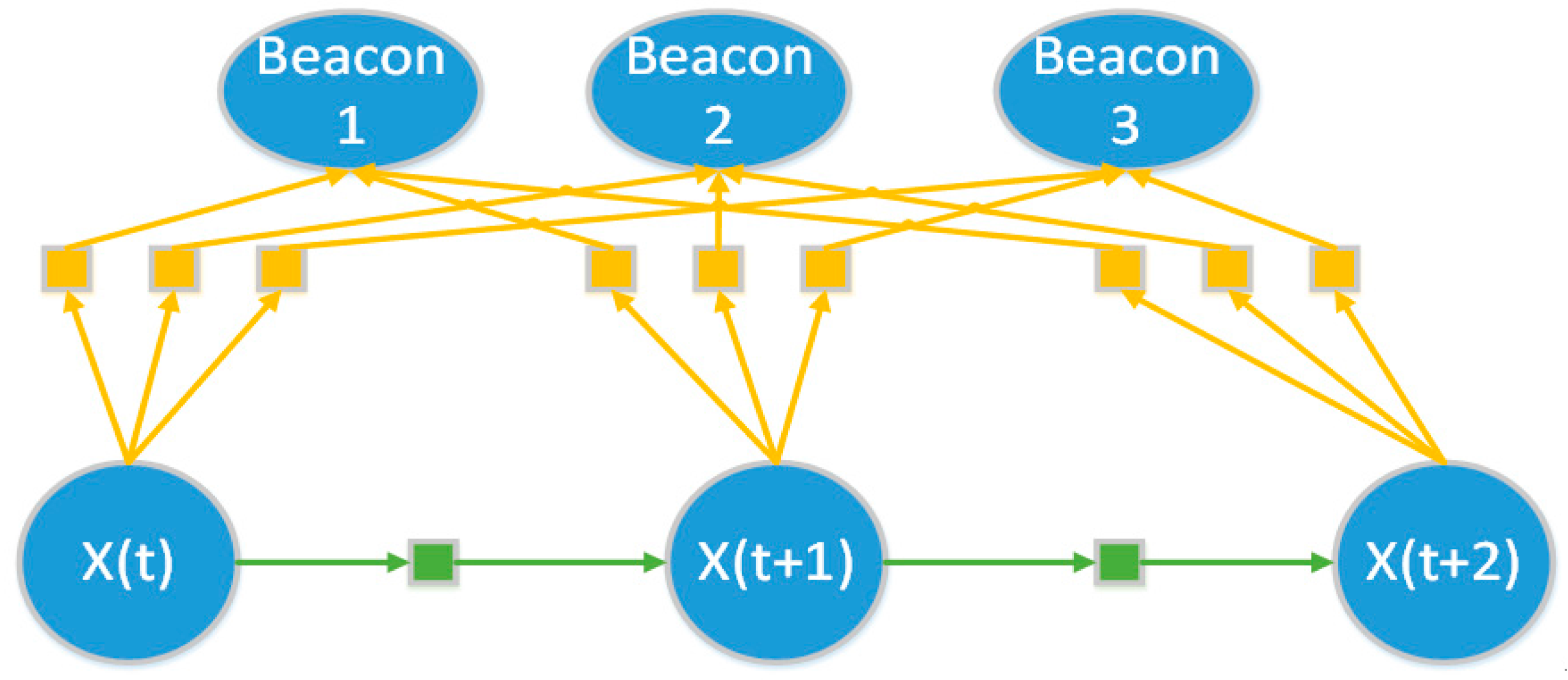
The graph optimization method is used in this paper to fuse the UWB and INS data. It first involves formulating the UWB/INS fusion-based positioning problem as a graph. The model constructed in this paper is shown in Figure 4, where there are two types of vertices. The first type of vertex corresponds to a UWB station and is represented by a blue ellipse in the figure. The information contained in this type of vertex is the 3-D coordinates of the UWB station, and its degree of freedom is 3. The status of the kth beacon vertex is denoted by . The second type of vertex is the virtual status vertex. Zero-speed detection is performed via the IMU. The posture that an IMU exhibits when the foot lands is defined as a vertex, and is represented by the blue circle in the figure. The information contained in this type of vertex, which is denoted by a four-element tuple, is the 3-D coordinates of its location and the status. The degree of freedom is 6, and the status of the ith status vertex is denoted by . The data from the UWB and INS sensors are used to form respective edges to represent the constraint on each vertex.
a. UWB-Measurement-Based Edge
First, we consider an easy scenario, where the UWB data are used to form a distance-constraining edge represented by the yellow lines in Figure 4. The measurement from the UWB sensor is the distance between Beacon and Tag. Let denote the measured distance between the ith status vertex and the kth beacon vertex. To construct a graph optimization model, we need to define a cost function:
Because only the distance constraint is considered, the elements in the status of the status node that describe posture are no longer useful. For clarity of presentation, can be divided into two parts: , where denotes the coordinates. and denotes the posture, which is a four-element tuple. After simplification, the cost function of the distance-constraining edge can be written as:
where denotes the operation of computing the vector modulus. Note that the error function in the graph-optimization-based method uses the measurements of UWB in 3D directly. In addition, there is a method for dynamically determining the information matrix of the UWB-measurement-based edge, which is discussed in Section Method for Dynamically Determining the UWB Confidence Level.
b. Edge Based on Adjacent ZUPT Gait Relations
Now, we discuss the edge between the status node at j and the status node at i, which is represented by the green lines in Figure 4. This type of edge computes the integral of INS, performs zero-speed detection to obtain the constraint that the speed is zero, and then outputs the observation as the final result. Let denote the observation. Because this constraint is applicable only to the vertex of the current moment and the vertex of the previous moment, there is only one possibility: .
The cost function can be defined as:
where denotes the set of distance metrics in SE(3). Consider the right distance metrics, namely, and
where denotes the matrix logarithm. In the form of a sequence expansion, it can be written as:
where denotes the inverse operation of the skew-symmetric operator, which produces a vector. After calculating the modulus, we can obtain the distance measurement.
Note that and are elements in , and no definition of addition is directly available because the sum of elements in does not necessarily belong to . An alternative is to transform and into a Lie algebra, perform the Lie-algebra additive operation, and then transform the result to . Section Method for Dynamically Determining the ZUPT Confidence Level covers the method for dynamically determining the information matrix for this type of edge.
Method for Dynamically Determining the ZUPT Confidence Level
We accumulatively compute the posture and coordinates of the IMU through integration. The system posture is usually described by a four-element tuple in this method to simplify the calculations, because the use of the four-element tuple can reduce the computational load. The Runge-Kutta method updates the tuple by computing the integral through the collected angular speed [25]. Let denote the four-element tuple that describes the posture. Consider an interval of . The updating formula can be written as
This formula intrinsically causes serious error in the case of a large angular speed, thereby resulting in grave error in the integration of the posture exhibited during walking and turning. It has been learned from real-world applications that the ZUPT positioning method is very accurate for straight lines. Error mainly occurs in the angle estimation. A slight error in angle may be magnified after a segment of a straight line, thereby causing glaring overall positioning error. A low confidence level can be allocated to the corner to improve the overall positioning accuracy and the algorithm’s sensitivity to the corner.
The variation of the IMU’s direction in the x-o-y plane is used in this paper to check whether the angle changes violently at the current moment. The confidence level of the current estimate is reduced if a large angular variation is detected. In this way, we can quickly correct the error of the IMU at the corner using the UWB observation, because the relative magnitude of UWB’s covariance matrix is larger, even if the absolute confidence level has not changed.
The experimental results in Section 3.2 will demonstrate the ability of this method to improve the positioning accuracy.
Method for Dynamically Determining the UWB Confidence Level
UWB produces no accumulative error during UWB/INS fusion and this is very instrumental in limiting the error accumulation of INS. Ideally, the accuracy of the UWB sensor is on the order of magnitude of decimeters. However, the accuracy of the UWB sensor is usually reduced due to various real-world factors, such as ambient temperature, power supply stability, fixed obstacles, the moving body and object, and even the body to be positioned. Therefore, the UWB sensing accuracy is not stable in practice and varies with location and time.
This leads to the following problems: If a low confidence level is allocated to all UWB observations, the high sensing accuracy of UWB is not fully exploited most of the time. However, allocating a high confidence level to all UWB observations will destabilize the positioning results and make it impossible to correct highly erroneous UWB observations using the IMU data. Moreover, because the UWB sensing accuracy varies with the environment, the confidence level should be adapted to the current scenario to ensure high positioning accuracy, which limits the application scope of UWB sensors.
To address these problems, we estimate the measurement accuracy using the residual of the optimization result that was obtained in Section 2.1, i.e., the obtained minimal value of . Consider the most common scenario, which is shown in Figure 5, where only one beacon produces very erroneous measurements, and the UWB measurements are usually larger than the actual distance [26]. Without loss of generality, it is assumed that only Beacon 1 is erroneous. Under this scenario, the sum of the errors in the measurements is
Consider a position distant from the Beacon. The circle’s radius is so large that the intersection of the three circles in the figure can be approximately regarded as a triangle. Because the radius is undoubtedly perpendicular to the circumference, it can be inferred that the circle is approximately perpendicular to the side of triangle. Therefore, is approximately equal to the sum of the distances between the real coordinates and each of the triangle’s sides.
The optimization result should be a point within the triangle. Because its radius is approximately perpendicular to the triangle’s side, it can be inferred that the cost function is approximately equal to the sum of the distances between this point and each of the triangle’s sides. Based on the geometric relationship that the sum of the distances between any point within the triangle and the triangle’s sides is fixed, we can approximately establish an equivalence relationship as
With this relationship, we can determine the information matrix of UWB measurements by substituting the minimized cost function for the measurement error. The observation of the UWB cost function is a 1-D variable; thus, the information matrix can be directly defined as follows:
Section 3.3 analyzes the relationship between the UWB signal’s optimized residual and the sum of measurement errors, and identifies a strongly linear relationship when the distance is large. Section 3.5 compares the influences of this method on the positioning accuracy under different scenarios and discovers the ability of this method to greatly improve positioning accuracy in complex scenarios.
3. Experimental Results and Analysis
3.1. Experimental Method and Scenario
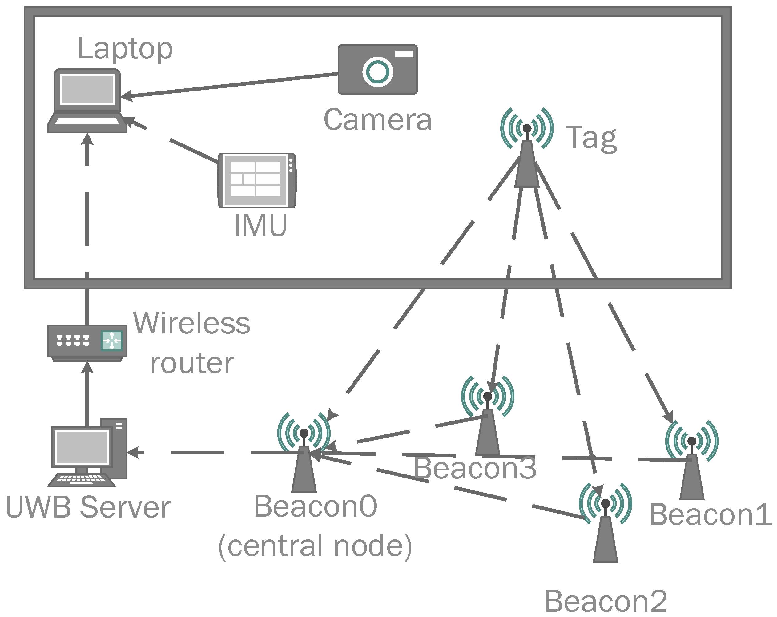
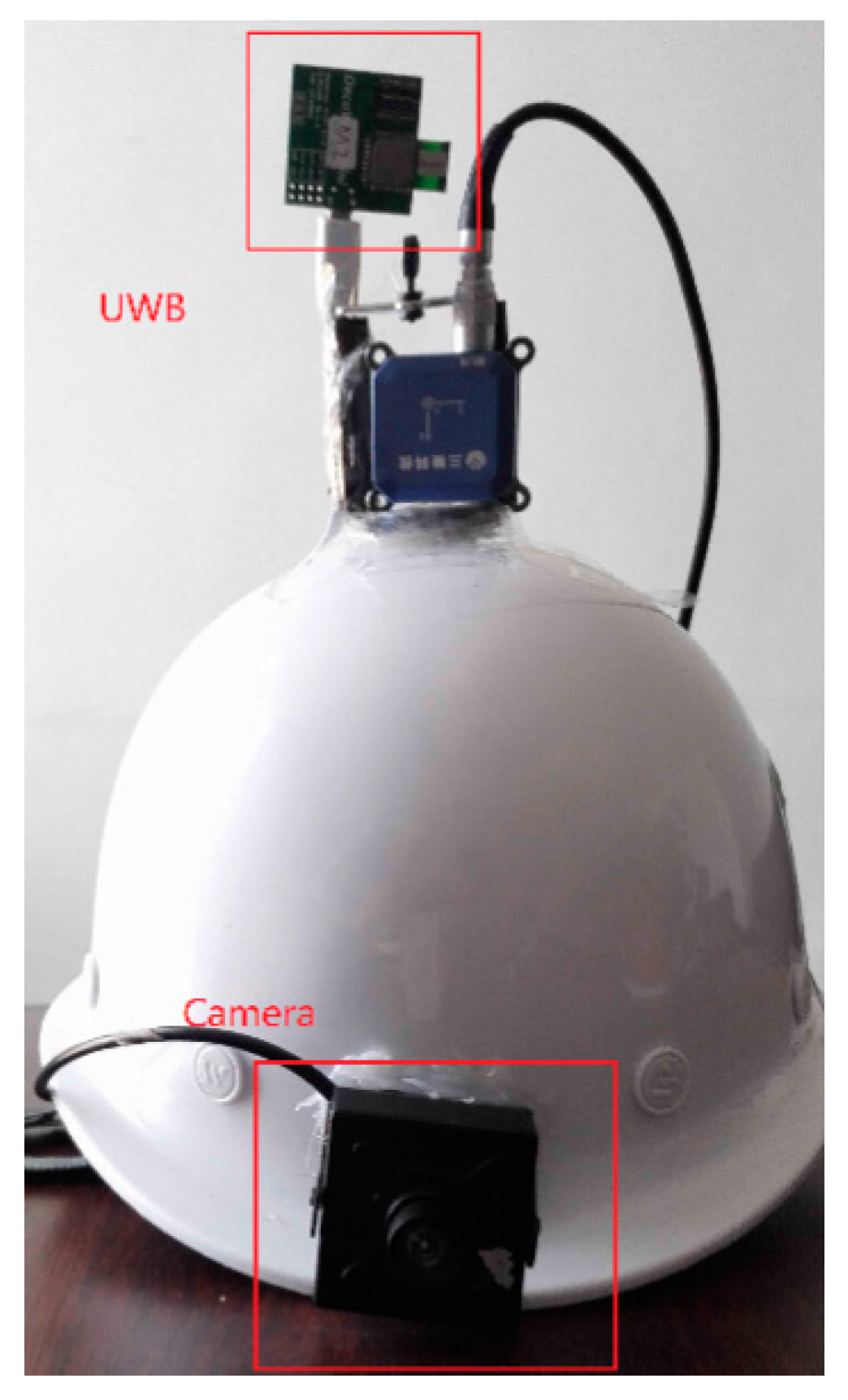
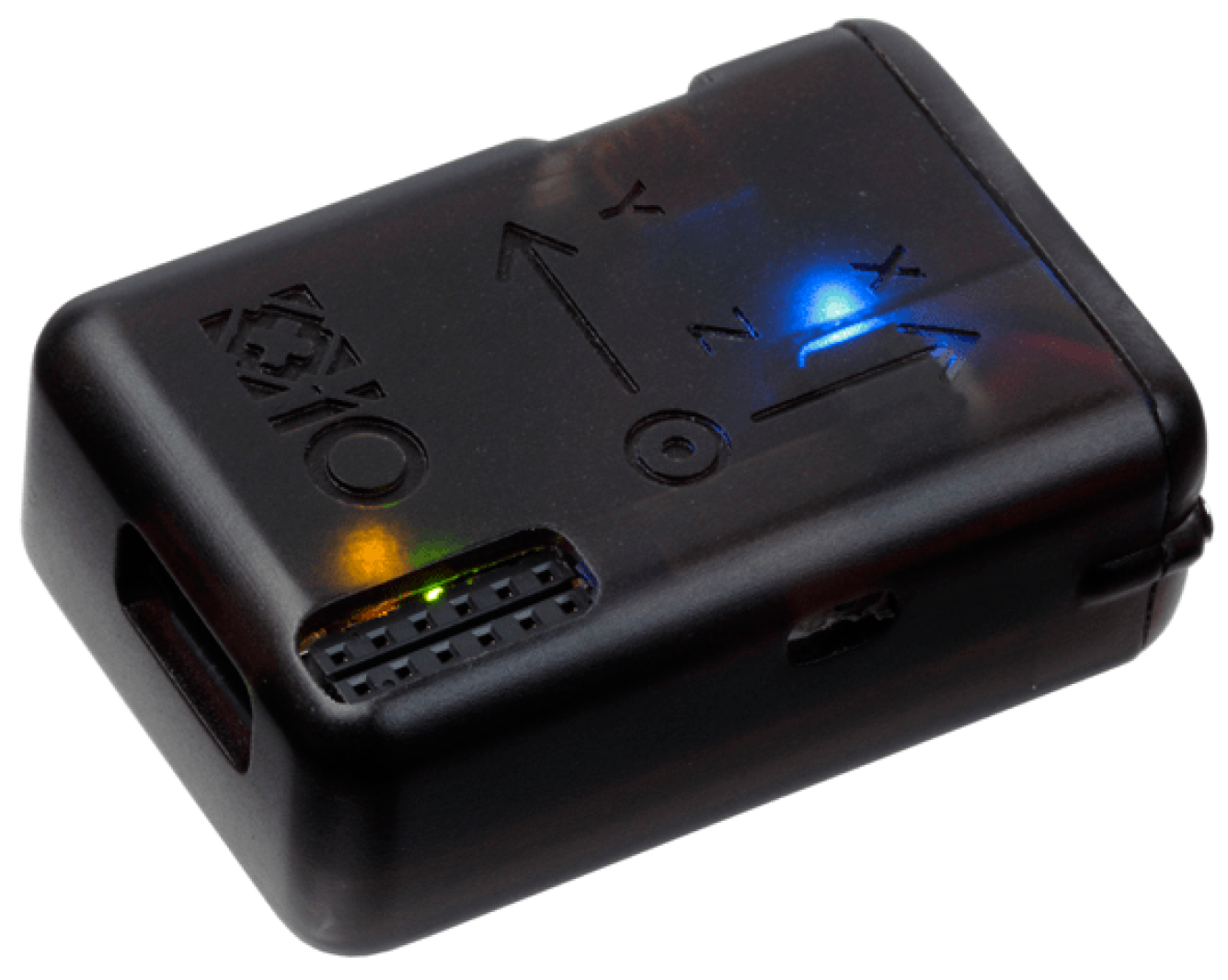
The experiment is performed in a hall with two load-bearing pillars as the major fixed obstacles, whose locations will be labeled in the subsequent tracking figure. The experimental devices include a UWB positioning system (four stations, namely, Beacon 0–Beacon 3, a positioning tag, and a UWB server responsible for receiving and pre-processing the UWB data), a camera, a foot-mounted IMU, a laptop, and a wireless router, which is responsible for providing a wireless network. The data transmission directions are shown in Figure 6, where a solid line indicates a wired connection and a dotted line indicates a wireless connection. Each beacon measures its distance from the tag, and the data are transmitted to the UWB server via Beacon 0. The UWB server pre-processes the data and delivers the data to the laptop via the WiFi network. The camera is directly connected to the laptop via USB and its data are used to provide the actual track. The camera determines the location of an object through ArUCO and its accuracy reaches approximately 7 cm after back-end optimization [27]. The foot IMU is connected to the laptop through Bluetooth to upload the 6-DOF data (acceleration and angular speed along the three axes). The laptop is responsible for data collection and time synchronization using the time stamps of the data. The camera and tag are installed at the head, as shown in Figure 7, and the IMU is installed at the foot, as shown in Figure 8.
The camera has a resolution of 1080 × 1920 and a frame rate of 30 FPS. Other parameters of the camera are also calibrated. The UWB chip is a DWM1000, which has an operational frequency of 3.5~6 GHz and an ideal positioning accuracy of 3 decimeters. The UWB system returns the distance measurement results at 2 Hz during the experiment. The IMU sensor is an MPU9250-based XIMU, which outputs data at a frequency of 128 Hz.
Three paths are tested in the experiment. In the first path, the object moves directly around the hall three times while trying to ensure the smoothness of the track. This path forms a rectangle. The second path is similar to the first, but involves more turns and passes through some regions that cause serious errors. The third path is characterized by small changes of angles during normal walking, changes of speed and short-term pauses in some regions. The ground truths of the first and second paths are presented in Section 3.4, while the ground truth of the third path is presented in Section 3.5.
Another experiment is conducted for performance evaluation in an underground parking which is a typical realistic scenario. In Section 3.6, trajectories of each algorithm with or without enough beacons have been tested.
3.2. Relationship between Attitude Change and Transform Change
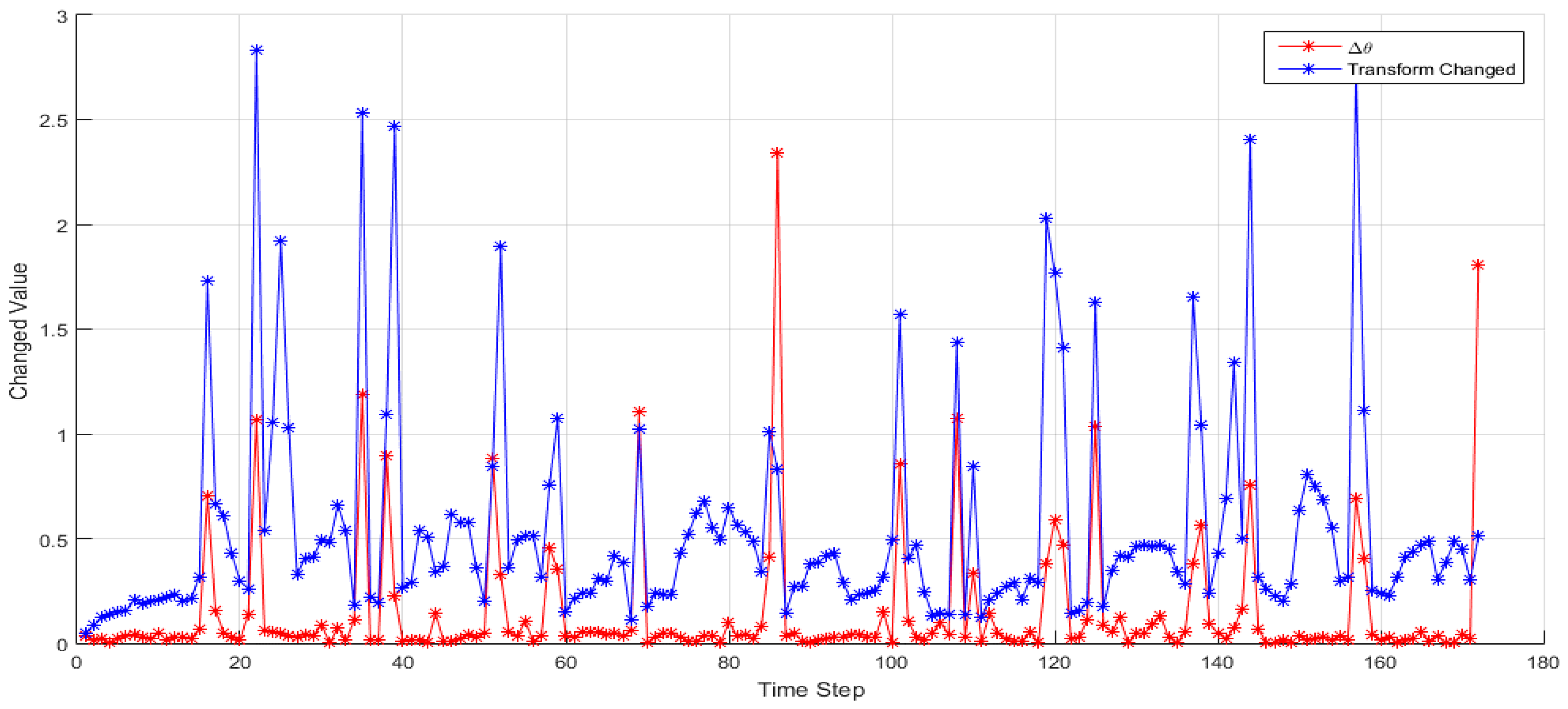
As mentioned earlier, the ZUPT algorithm usually produces significant error when the angular speed is large. That is, these grave errors occur at turns. To better understand this phenomenon, we compare the original constraint and the optimization result along the second path. Figure 9 shows the variations in Transform after graph optimizations that correspond to angular changes, where denotes the change of the IMU’s orientation in the xoy plane in units of rad, and the unit of the y-axis is also rad. Transform Changed denotes the difference in the relationship between two nodes after optimization, where the relative relationship is directly obtained using the ZUPT algorithm. Let and denote the location and posture of the two nodes, which are represented by a transform matrix, after optimization. The relative relationship between the two nodes can be represented by . Here, is the relative relationship, which is directly obtained using the ZUPT. The data labelled Transform Changed in this figure represent the difference. Note that to present the results more intuitively, the scale of the output results has been adjusted to guarantee that they are of the same order of magnitude as .
According to the figure, the larger the angular variation, the larger the variation in Transform Changed. Because the optimization result is very close to the ground truth, it is inferred that Transform Changed indirectly reveals the difference between the value of which is produced by ZUPT, and the ground truth. Therefore, we conclude that the error of ZUPT at each step is large when the angular variation is large. This indicates that it is feasible to dynamically determine the confidence level of ZUPT results using the angular variation. Because a better-estimated value for the covariance matrix of the ZUPT edge is obtained, more accurate positioning can be achieved.
3.3. Relationship between the UWB Measurement Error and the Optimization Residual
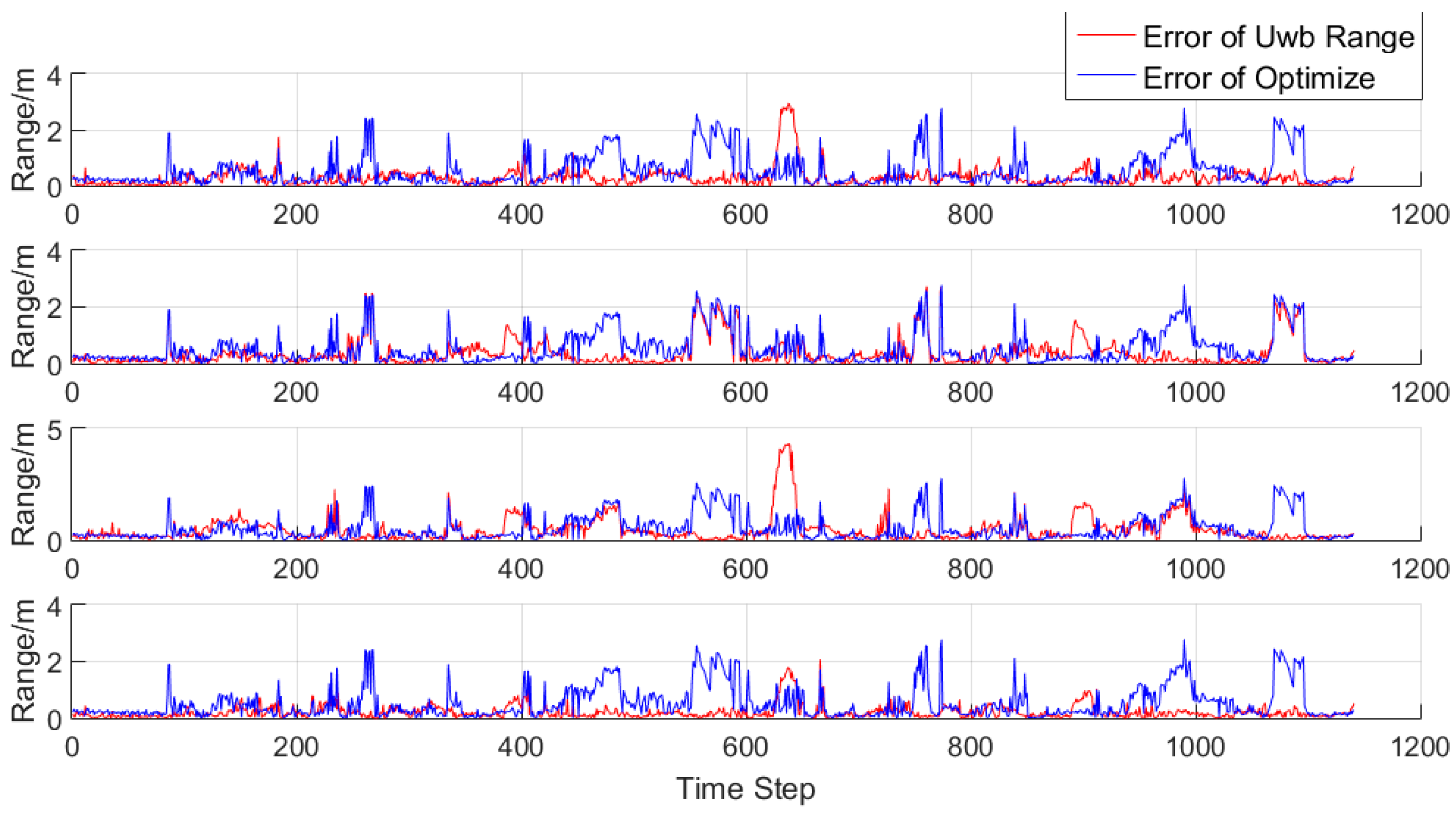
Previously, we used the geometrical relationship to predict the relationship between the UWB optimization residual and the UWB measurement error, and concluded that they should be roughly equal. However, this conclusion is valid only if we simplify the three stations and make several approximations in the typical scenario. To support this conclusion, we computed the deviation of UWB measurements from the track obtained using the visual algorithm. The red line in Figure 10 shows the absolute values of the measurement errors of the four stations, and the blue line denotes the optimization residuals. Note that the four stations share the same optimization residuals. The UWB sensor is highly accurate and only one station produces erroneous measurements for most stages of the process. By examining the relationship between the UWB measurement error and optimization residual, we find that the latter is strongly correlated with the former. That is, the optimization residual is large when the UWB measurement error is large, and the optimization residual is small when the UWB sensing data are accurate.
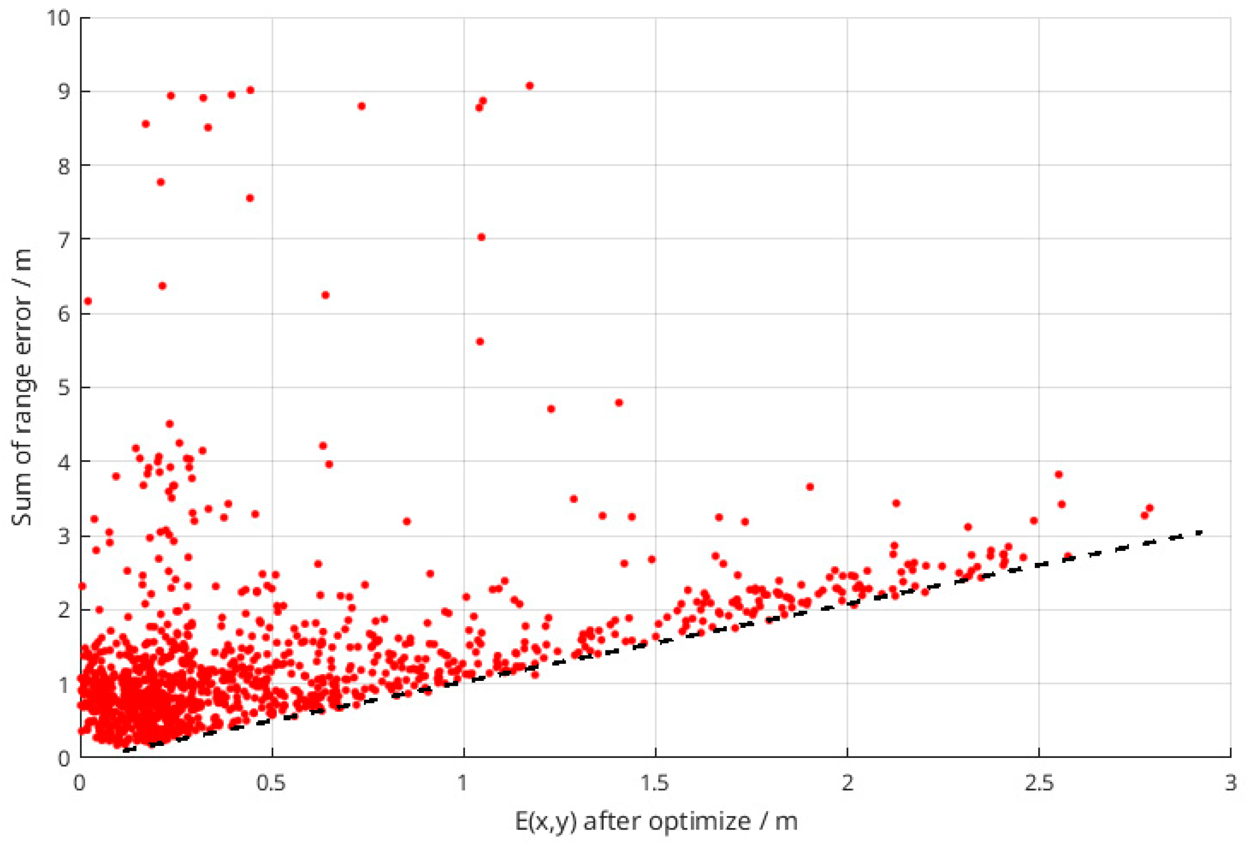
The optimization residual effectively indicates the lower bound of the sum of the measurement errors. As shown in Figure 11, the abscissa represents the optimization residual in m and the ordinate represents the sum of the measurement errors in m. The red scattered points denote the data points that were collected in the experiment, and the black dotted line is an auxiliary line with a gradient of 1. Because the points on the auxiliary line represent the moments at which the optimization residual and the sum of the measurement errors are equal, most data points fall above the line. Thus, given an optimization residual, the lower bound of the sum of the measurement errors is equal to this optimization residual. Therefore, it is feasible to determine the confidence level of UWB measurements using the optimization residual.
3.4. Comparison of Graph-Fusing with Other Methods
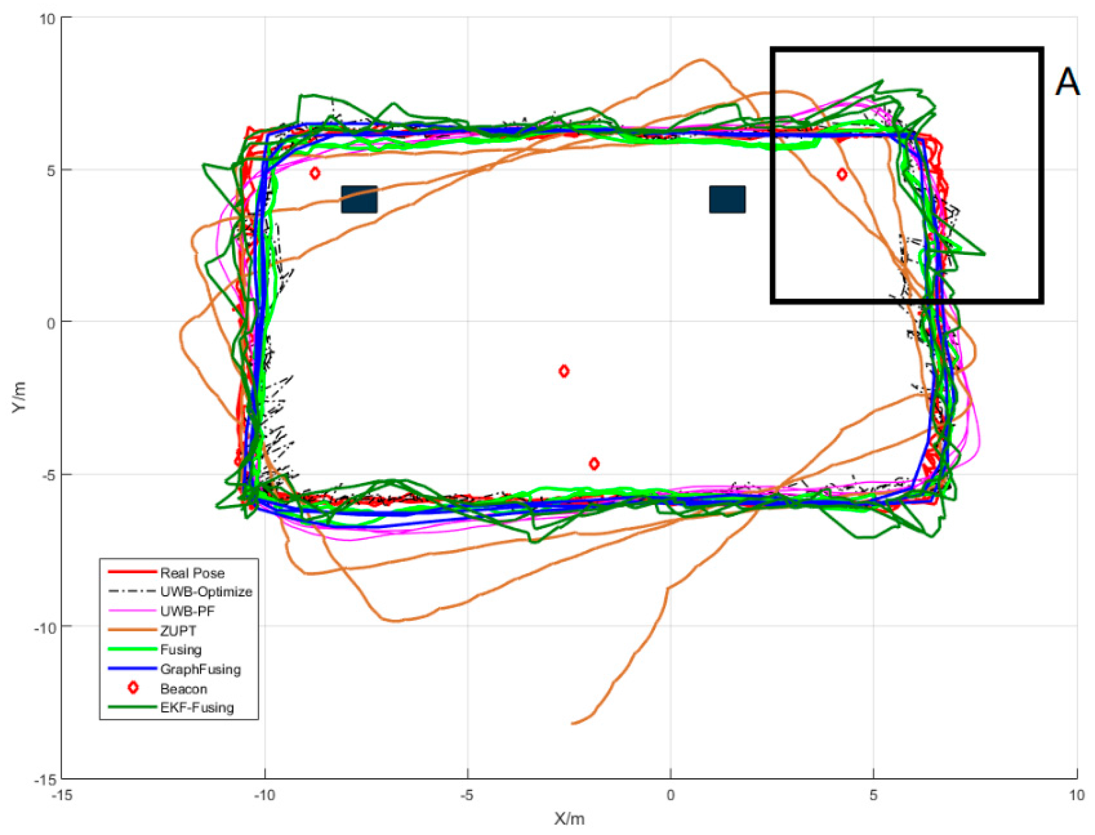
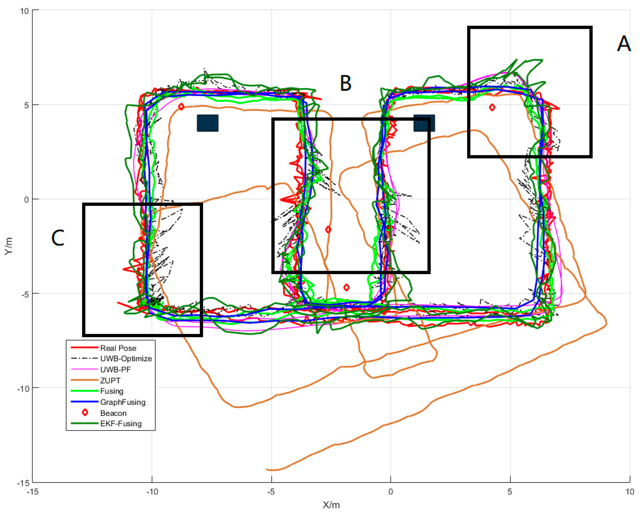
To evaluate the performance gain of GraphFusing, it is compared with the following methods: the IMU-based ZUPT positioning algorithm (ZUPT), the pure UWB positioning algorithm based on minimization of the error function (UWB-Optimize), the pure UWB positioning algorithm based on particle filtering (UWB-PF), the UWB/INS fusion algorithm based on particle filtering (Fusing), and the UWB/INS fusion algorithm based on EKF (EKF-Fusing) [7]. Figure 12 shows the positioning performances of all these methods for the first path. The black rectangles denote the obstacles. The ground truth, which was obtained through visual positioning, is denoted by RealPose in the figure. The object starts in the lower-left corner and then moves clockwise along the first path for three rounds. Figure 13 shows the positioned track of each algorithm for the second path. The second path shares the same starting point and moving direction as the first path, but an extra track is added, which has serious UWB errors. The object moves at almost constant speed during the experiment; its movement is quite smooth when it moves in a straight line and tries to turn at a right angle. The initial value for all the algorithms is determined by the ground truth, and the initial orientation of ZUPT is determined by the moving direction of the ground truth for the previous five seconds.
To optimize the performances of the two algorithms based on particle filtering, we increase the number of particles to 5000. Note that further increasing the number of particles is no longer helpful in increasing the particle filter’s positioning accuracy. The performance of the EKF-Fusing method has been optimized through the choice of parameters, such as the covariance matrix of observation measurements and system noise. The two methods that were proposed above for dynamically determining the confidence level are used to improve the positioning accuracy of GraphFusing.
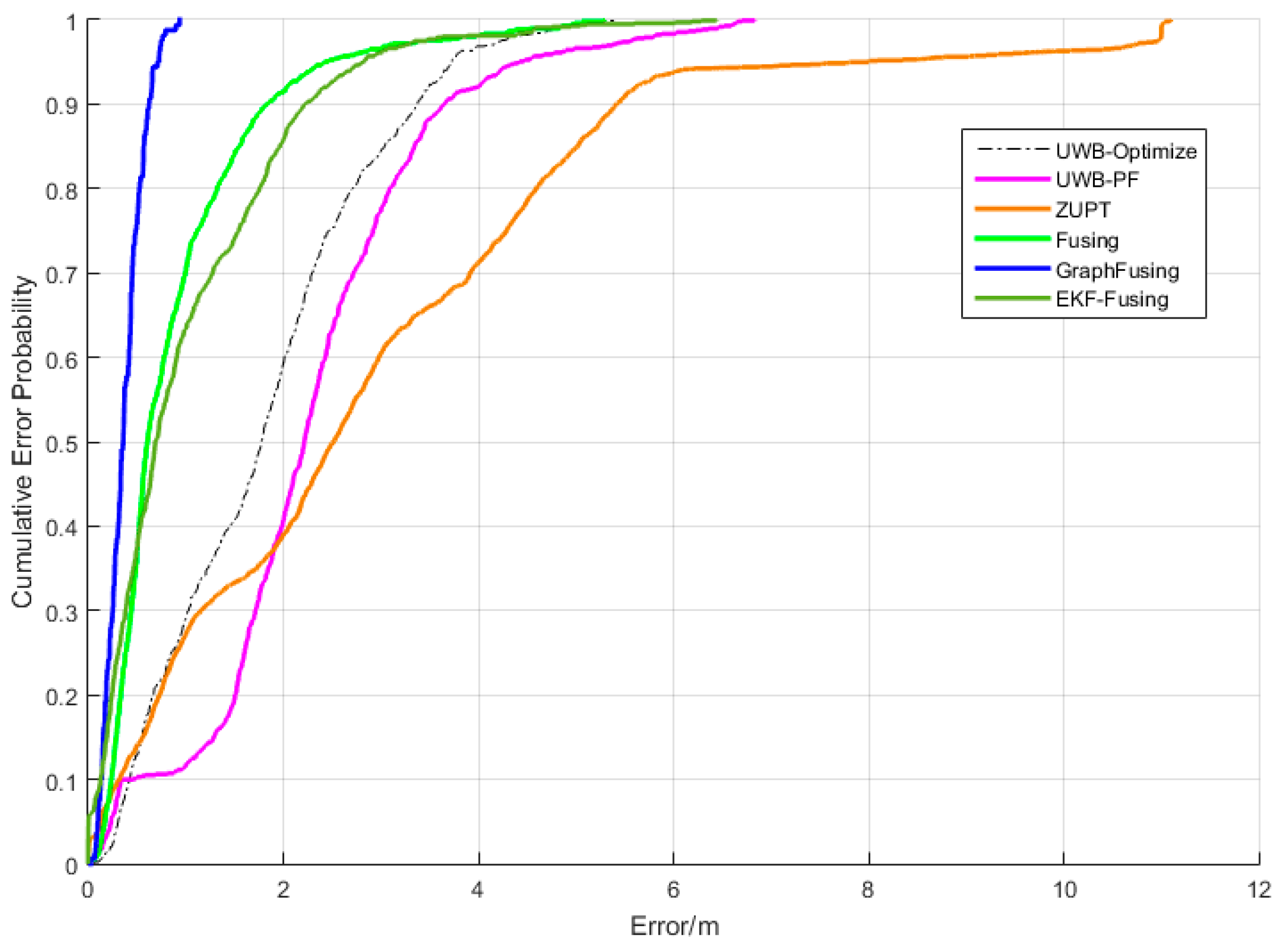
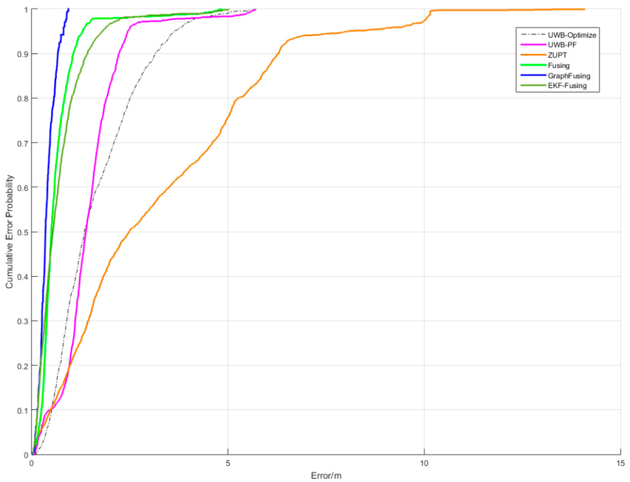
According to the results, for each of the two paths, ZUPT is very accurate in positioning the straight line, but it produces serious error when estimating the turning angle. This is consistent with the discussion above. The effect of the grave error of ZUPT can be reduced by decreasing the confidence level of the results output by ZUPT. UWB-Optimize is chosen here to indirectly determine the error of each UWB measurement at each moment and the overall deviation. By incorporating speed and moving speed into the positioning process, UWB-PF tries to ensure uniform linear motion. Therefore, the track produced by UWB-PF is very smooth throughout the positioning process. UWB-PF is very accurate when the UWB error is small or of short duration. However, due to its use of UWB sensors only, UWB-PF cannot fix the position accurately when the error is large or of long duration. According to Figure 14 and Figure 15, EKF-Fusing, Fusing and GraphFusing are more accurate than the other methods, and GraphFusing is vastly superior to Fusing and EKF-Fusing in terms of accuracy. Hence, GraphFusing is mainly compared with Fusing in the remainder of this paper.
The analysis of the results for the first path indicates that the Fusing algorithm, which fuses the IMU data, considerably reduces the local error of the UWB signal. Even when the data anomaly persists for a relatively long time, the Fusing algorithm is highly accurate after benefiting from the IMU data. When errors occur in the UWB data, the particle filter tries to estimate the status’s maximum posterior probability using many scattered particles. Because its particles utilize only the status of the previous moment and the IMU input of the current moment, the weights of the particles close to the global minimum will be increased enormously. However, the output positioning result remains accurate because many particles are close to the real value when computing the weighted average. However, the generated track fluctuates substantially. The track generated by GraphFusing is both accurate and smooth in comparison.
The UWB signal throughout the second path is more complex than that for the first path and the second path includes more turns. A comparison between the two paths effectively reveals two shortcomings of the particle-filter-based positioning algorithm.
The first shortcoming of the Fusing algorithm can be identified by comparing the positioning results in rectangle A in Figure 12 and Figure 14. The UWB-Optimize algorithm produces similar errors for this region along the two paths. However, the positioning results of the Fusing algorithm vary wildly. This is because the particle filter (and other filters) incorporates the constraints of all the previous statuses into several status variables, namely, the coordinate, speed and direction in this paper. Consider the scenario in which the object has just made a turn in the second path. Although an accurate positioning result is achieved quickly due to the consistency between the UWB signal and the IMU output, the individual particles are not set to the same moving direction. Therefore, when the maximal value of the UWB observation model’s likelihood function is biased towards one of the previous moving directions, the particles whose moving directions have not converged to the true direction will have a large likelihood probability. Consequently, the results drift towards these particles. Consider the example presented in this paper. The moving direction before the turn in region A is the positive direction along the Y-axis, and the moving direction after the turn is the positive direction along the X-axis. Although the overall moving direction has been corrected to the correct X-axis positive direction after the turn, some particles still move along the Y-axis positive direction. However, before this turn in the middle of region A, the maximal value of the UWB observation model’s likelihood function is biased towards the Y-axis positive direction (as shown in the track of UWB-Optimize), and these particles have a large likelihood probability. Therefore, the Fusing algorithm produces greater errors for the second path.
The positioning results for region C in Figure 14 provide evidence of this inference. Because the maximal value of the UWB observation model’s likelihood function is opposite to the moving direction, even when the UWB observation is highly erroneous, the positioning error of the Fusing algorithm is limited. Desirably, GraphFusing exhibits the reverse property because it constrains the current positioning result by directly using the information of previous moments, thereby eliminating the need to compress the series of previous statuses. Instead of stabilizing the positioning result through several rounds of iteration after the turn is made, GraphFusing produces a stable result based on a series of observations. This enables GraphFusing to respond to changes more quickly. Meanwhile, GraphFusing can utilize the relative displacement, which is accurately computed by the IMU, in a more direct manner to fully exploit the positioning results of the IMU, which are extremely accurate over short periods of time.
Another shortcoming of the Fusing algorithm is revealed by the results for rectangle B in the figure, where a grave error occurs with the UWB-Optimize algorithm. Due to the long-term continuous existence of errors, Fusing cannot guarantee that the previous status information, which consists of the speed and direction, effectively constrains its positioning result. However, the GraphFusing algorithm considers the information over a series of previous statuses, and the errors that occur at the turn are corrected by the accurate UWB observations. The short-distance grave errors of UWB do not lead to a deviation of the positioning results from the real track. Moreover, the subsequent errors in the opposite direction may further guarantee the correctness of the moving direction.
The two shortcomings described above arise from the simplification of the previous status in the Fusing algorithm. The previous statuses are compressed into speed and moving direction. If a high confidence level is allocated to these elements of information, the Fusing algorithm will be unable to respond quickly to changes of speed or moving direction. Even when the data output by the IMU are available as a reference, the positioning accuracy still decreases because the IMU data are highly erroneous at the turning point. If a small confidence level is allocated to these elements of information, the positioned track will deviate quickly from the ground truth after errors occur in the UWB observation. GraphFusing provides an effective approach that solves this problem by explicitly incorporating the series of previous observations into the positioning process. However, because a sub-graph that consists of UWB data and ZUPT data for 24 steps is optimized at each moment for positioning, the computational complexity of GraphFusing is higher than that of UWB-PF. In our experiments, the calculations were performed on a machine equipped with an E3-1230 v2 CPU. On this machine, UWB-PF requires only 4.1 s to calculate the data sets (that might consume up to 107 s) even when there are 5000 particles, but GraphFusing takes 53.0 s to calculate the data sets. Therefore, the proposed algorithm is difficult to run on a micro controller in real time, but has an acceptable computational complexity for calculation on a CPU that is better than E3-1230 v2 in real time. It is worth noting that in practice, the calculation of each time step is complete 3 seconds after receiving the data.
3.5. Performance Comparison of the Two Confidence-Level Methods
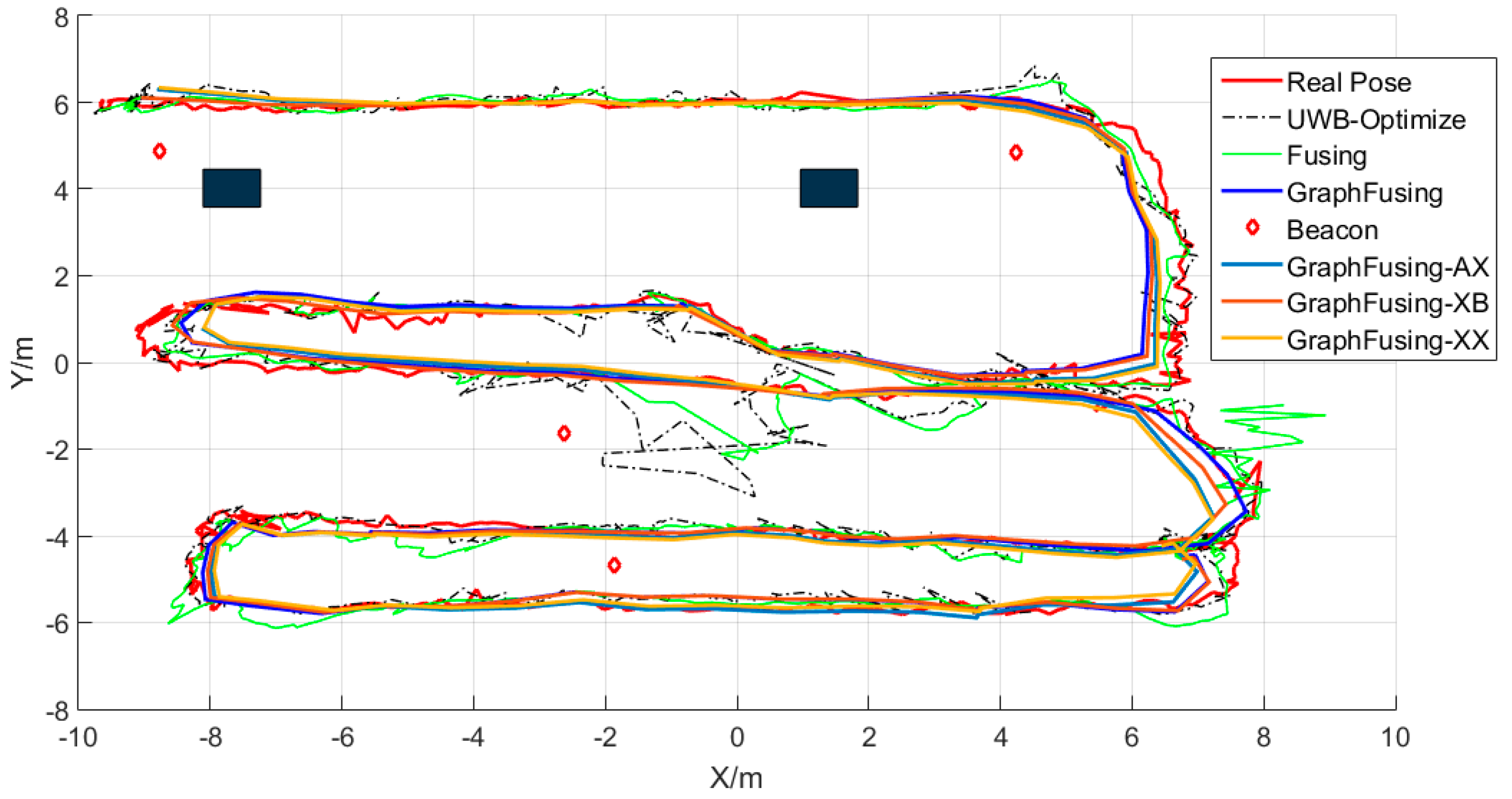
This subsection compares the influences of the two confidence-level methods on the positioning accuracy. To facilitate this illustration, we let A denote the ZUPT confidence-level method and let B denote the UWB confidence-level method. The GraphFusing algorithm adopts A and B at the same time; GraphFusing-AX adopts A and its UWB confidence level is fixed; GraphFusing-XB adopts B and its ZUPT confidence level is fixed; and GraphFusing-XX refers to the method in which the confidence levels are fixed for all sides.
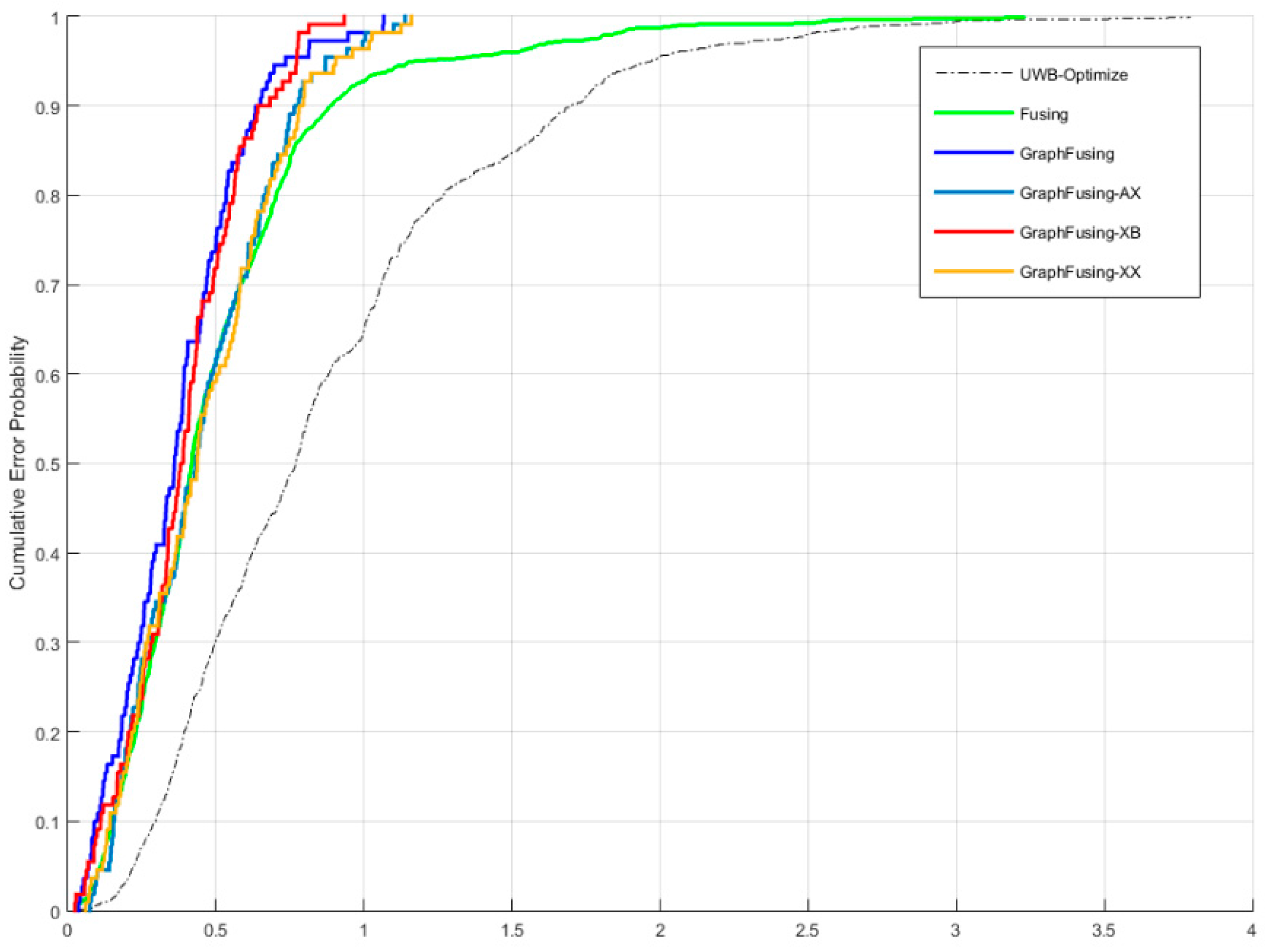
Figure 16 compares the positioned tracks of GraphFusing and Fusing under four scenarios along the third path. The track of UWB-Optimize is mainly used to indirectly indicate the quality of the UWB signal. The aim of the experiment along the third path is to evaluate the algorithm’s performance under a more complicated setting. To this end, the path involves many irregular turns, arcs, acceleration, and deceleration, and the tracked object sometimes halts directional movement and rotates in place. As shown in the figure, a section of the track from Fusing around the point (0, −1) deviates greatly from the ground truth and is close to the result of UWB-Optimize. This is because the object stays at this point for some time, and the positioning result of Fusing begins to become biased towards the maximal value of the likelihood function. It is difficult to differentiate among the positioning accuracies of the four GraphFusing algorithms. However, GraphFusing is generally more robust. Figure 17 shows the accumulative error distributions of the compared methods. Because the compared methods are mainly the four GraphFusing algorithms, it is not observed that the accumulative probability of Fusing reaches 1.0. The figure shows that GraphFusing is vastly superior to GraphFusing-XX in terms of accuracy. Although the accumulative probability of GraphFusing-XB for error below 0.8 m is larger than that of GraphFusing, GraphFusing maintains superiority over an error range that is smaller but more important.
To more intuitively reveal the differences in accuracy among the four GraphFusing variants, Table 1 compares the positioning errors of the four algorithms for the three paths. GraphFusing is highly accurate and its positioning accuracy further improves by a limited margin when it adopts the two confidence-level methods.
3.6. Performance Validation in Realistic Scenario
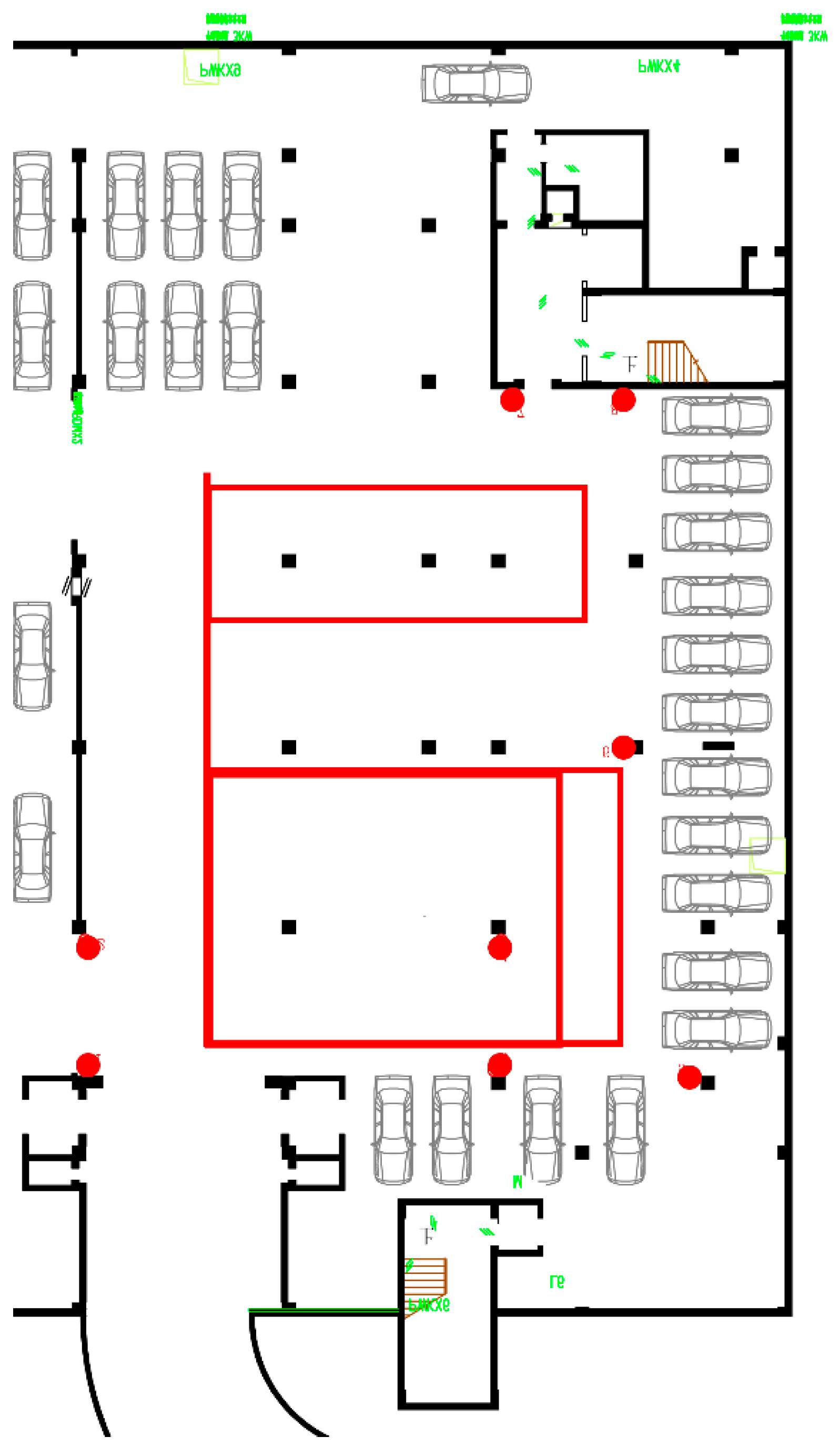
As mentioned earlier, the GraphFusing algorithm provides a better accuracy in the previous scenario. However, the situation, simple as that, may fall short of representation of the realistic scenario. Aiming to verify the performance of the GraphFusing algorithm, we conducted a new experiment in an underground parking, which is a typical scene in real applications. As shown in Figure 18, the red lines denote the reference path. Due to the complexity of the parking, it is difficult to provide a real position through using our vision-based positioning system. Therefore, the reference path is obtained through control points. Beacons, installed on the wall, are denoted as red circles. The black lines and rectangles denote wall and pillars, respectively. To verify the positioning accuracy of each algorithm under the conditions with or without enough beacons, we tested all algorithms in the two situations.
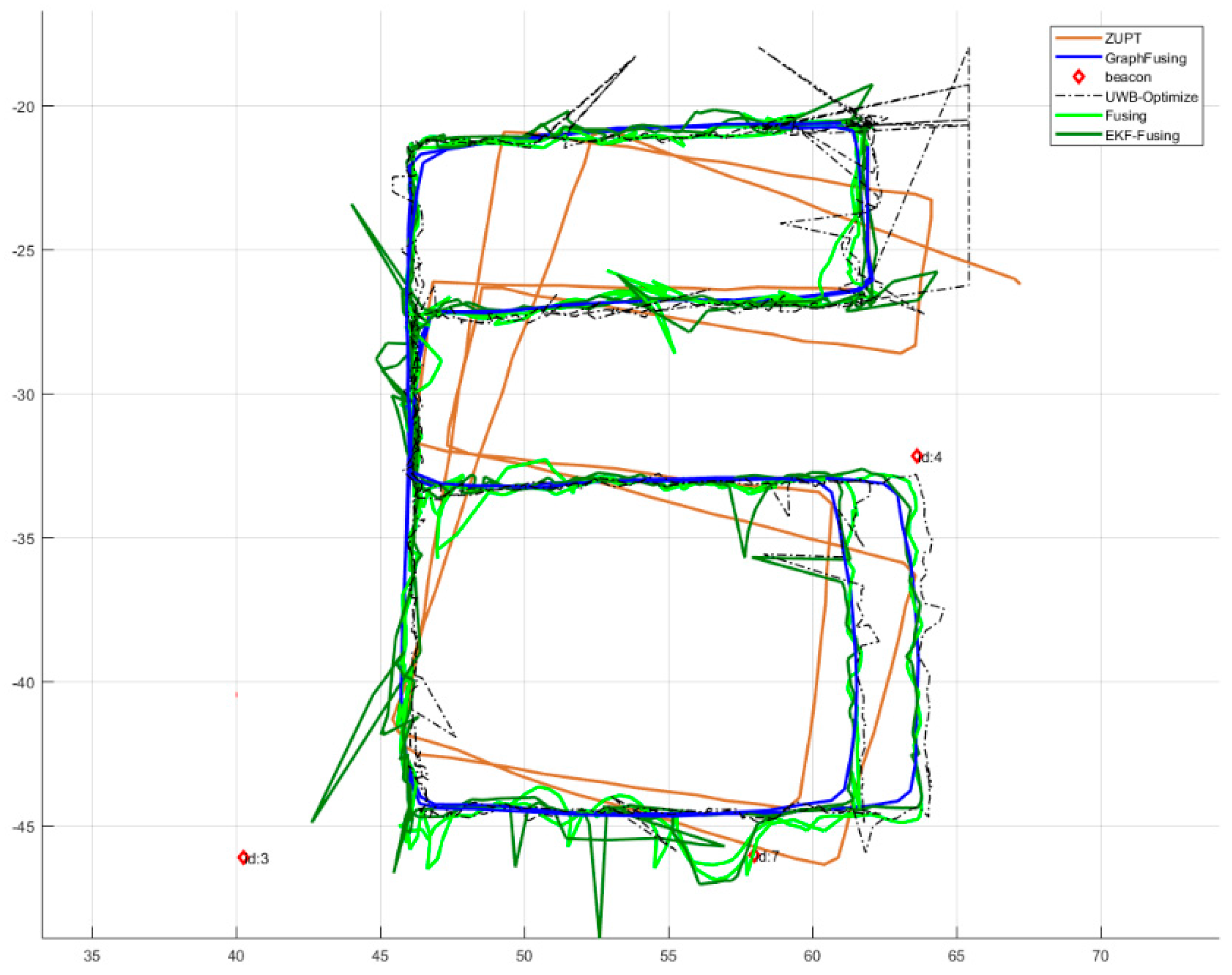
The result of all algorithms based on measurements of eight beacons is presented in Figure 19. Although without a real position as we provided in previous experiments, it is apparent that the accuracy of GraphFusing is higher than that of EKF-Fusing. Benefitting from the numbers of measurements, the trajectory of UWB-optimize, except for some outliers, has nearly approximated the real position. Meanwhile, the trajectory of the EKF-Fusing algorithm is not good enough, which might be caused by information loss in the measurement stage. In other words, a significant error will be generated under NLOS conditions when using a Gaussian distribution to approximate the probability distribution of the measurements with non-Gaussian noise. The higher accuracy of the Fusing algorithm provided additional evidence for this hypothesis, because the only difference between Fusing and EKF-Fusing is whether using a Gaussian distribution approximates the real distribution.
The result of all algorithms based on measurements of 3 beacons is presented in Figure 20. Although the total number of beacons could be very large in real applications, the number of UWB beacons in a certain sub-area is rarely more than 6, because it is unnecessary that provide more than 6 beacons. Actually, there are often only 3 beacons in a sub-area, which is enough to provide a position. In this situation, the adopted beacons can be observed in the figure. Because of the lack of measurements, the accuracy of UWB-optimize is lower than when using eight beacons. The accuracy loss of the Fusing algorithm, which can easily be found according to the paths, was caused by the loss of previous information. However, benefitting from the non-compressed information adopted in computation, the GraphFusing algorithm provides a good trajectory, especially compared to other algorithms. It is worth noticing that, the EKF-Fusing algorithm shows better accuracy than the previous situation that uses 8 beacons because the EKF-Fusing algorithm has a poor ability to process outliers. Meanwhile, there are many obstacles between the tag to the five other beacons in the whole trajectory, indicating that several anomalous measurements would be generated.
4. Conclusions
The graph optimization method is utilized in this study to directly incorporate the series of previous statuses and the relationships between statuses into the optimization process. It provides an approach to solving the problem of information loss by the traditional method that simplifies the series of previous statuses. Note that the confidence level of the previous status cannot be determined during the positioning process due to the loss of information. Assigning a high confidence level to the previous status makes it difficult to correct the error in the track and leads to a slow response to rapid change, while assigning a low confidence level to the previous status makes the algorithm susceptible to erroneous observations. By completely preserving the series of previous statuses, the graph-optimization-based fusion method can effectively process the relationship between the current status and the previous status and achieves a considerable improvement in accuracy. The methods for dynamically determining the confidence levels of the UWB and ZUPT observations are presented to further improve the positioning accuracy. Higher positioning accuracy is achieved through the application of the algorithm described above. However, the graph optimization method has an obvious shortcoming compared to Bayes filtering: large computational complexity. To improve the speed of the graph optimization algorithm, at least two approaches could be adopted in the future. First, because the system states are not significantly different from the previous states at most moments of the positioning process, an incremental optimization method could be applied to speed up the method by linearizing only parts of the cost function. Second, the positions from EKF and PF are sufficient, in most cases, when the measurements are reliable. Thus, the graph-optimization-based algorithm need not calculate at every moment when the measurements are received. Hence, the graph-optimization-based algorithm could function as a possible tool for improving the accuracy of the ZUPT/UWB positioning system.
Acknowledgments
This work was supported by the Fundamental Research Funds for the Central Universities under grant number 2017XKQY020.
Author Contributions
Yan Wang and Xin Li conceived, designed and performed the experiments; Yan Wang analyzed the data and wrote the paper.
Conflicts of Interest
The authors declare no conflicts of interest.
References
- Dardari, D.; Closas, P.; Djuri, P.M. Indoor Tracking: Theory, Methods, and Technologies. IEEE Trans. Veh. Technol. 2015, 64, 1263–1278. [Google Scholar] [CrossRef]
- Kok, M.; Hol, J.D.; Schon, T.B. Indoor positioning using ultrawideband and inertial measurements. IEEE Trans. Veh. Technol. 2015, 64, 1293–1303. [Google Scholar] [CrossRef]
- Fan, Q.; Sun, B.; Sun, Y.; Wu, Y.; Zhuang, X. Data Fusion for Indoor Mobile Robot Positioning Based on Tightly Coupled INS/UWB. J. Navig. 2017, 70, 1079–1097. [Google Scholar] [CrossRef]
- Wang, H.; Lenz, H.; Szabo, A.; Bamberger, J.; Hanebeck, U.D. WLAN-Based Pedestrian Tracking Using Particle Filters and Low-Cost MEMS Sensors. In Proceedings of the WPNC ‘07 4th Workshop on Positioning, Navigation and Communication, Hannover, Germany, 22 March 2007. [Google Scholar]
- Chai, W.; Chen, C.; Edwan, E.; Zhang, J.; Loffeld, O. 2D/3D indoor navigation based on multi-sensor assisted pedestrian navigation in Wi-Fi environments. In Proceedings of the Ubiquitous Positioning, Indoor Navigation, and Location Based Service (UPINLBS), Helsinki, Finland, 3–4 October 2012. [Google Scholar]
- Bahillo, A.; Angulo, I.; Onieva, E.; Perallos, A.; Fernández, P. Low-Cost Bluetooth Foot-Mounted IMU for Pedestrian Tracking in Industrial Environments. In Proceedings of the 2015 IEEE International Conference on Industrial Technology (ICIT), Seville, Spain, 17–19 March 2015. [Google Scholar]
- Zampella, F.; De Angelis, A.; Skog, I.; Zachariah, D.; Jimenez, A. A constraint approach for UWB and PDR fusion. In Proceedings of the 2012 International Conference on Indoor Positioning and Indoor Navigation (IPIN), Sydney, NSW, Australia, 13–15 November 2012. [Google Scholar]
- Lim, J.; Lee, K. Integration of Pedestrian DR and Beacon-AP based Location System for Indoor Navigation. In Proceedings of the International Global Navigation Satellite Systems Society IGNSS Symposium, Gold Coast, QLD, Australia, 16–18 July 2013. [Google Scholar]
- Ban, R.; Kaji, K.; Hiroi, K.; Kawaguchi, N. Indoor positioning method integrating pedestrian dead reckoning with magnetic field and wifi fingerprints. In Proceedings of the 2015 Eighth International Conference on Mobile Computing and Ubiquitous Networking (ICMU), Hakodate, Japan, 20–22 January 2015; pp. 167–172. [Google Scholar]
- Peltola, P.; Hill, C.; Moore, T. Particle filter for context sensitive indoor pedestrian navigation. In Proceedings of the 2016 International Conference on Localization and GNSS (ICL-GNSS), Barcelona, Spain, 28–30 June 2016; pp. 28–30. [Google Scholar]
- Kim, N.; Kim, Y. Indoor Positioning System with IMU, Map Matching and Particle Filter. In Recent Advances in Electrical Engineering and Control Applications; Springer: Berlin, Germany, 2015; pp. 41–47. [Google Scholar]
- Malyavej, V.; Kumkeaw, W.; Aorpimai, M. Indoor robot localization by RSSI/IMU sensor fusion. In Proceedings of the 2013 10th International Conference on Electrical Engineering/Electronics, Computer, Telecommunications and Information Technology (ECTI-CON), Krabi, Thailand, 15–17 May 2013. [Google Scholar]
- Yang, C.; Blasch, E. Kalman Filtering with Nonlinear State Constraints. IEEE Trans. Aerosp. Electron. Syst. 2009, 45, 70–84. [Google Scholar] [CrossRef]
- Georgy, J.; Karamat, T.; Iqbal, U.; Noureldin, A. Enhanced MEMS-IMU/odometer/GPS integration using mixture particle filter. GPS Solut. 2011, 15, 239–252. [Google Scholar] [CrossRef]
- Strasdat, H.; Montiel, J.M.M.; Davison, A.J. Visual SLAM: Why filter? Image Vis. Comput. 2012, 30, 65–77. [Google Scholar] [CrossRef]
- Engel, J.; Koltun, V.; Cremers, D. Direct Sparse Odometry. IEEE Trans. Pattern Anal. Mach. Intell. 2017, PP, 1. [Google Scholar] [CrossRef] [PubMed]
- Engel, J.; Usenko, V.; Cremers, D. A Photometrically Calibrated Benchmark For Monocular Visual Odometry. arXiv, 2016; arXiv:1607.02555. [Google Scholar]
- Mur-Artal, R.; Montiel, J.M.M.; Tardos, J.D. ORB-SLAM: A Versatile and Accurate Monocular SLAM System. IEEE Trans. Robot. 2015, 31, 1147–1163. [Google Scholar] [CrossRef]
- Hess, W.; Kohler, D.; Rapp, H.; Andor, D. Real-time loop closure in 2D LIDAR SLAM. In Proceedings of the 2016 IEEE International Conference on Robotics and Automation (ICRA), Stockholm, Sweden, 16–21 May 2016; pp. 1271–1278. [Google Scholar]
- Banerjee, S.P. Improving Accuracy in Ultra-Wideband Indoor Position Tracking through Noise Modeling and Augmentation. Ph.D. Thesis, Clemson University, Clemson, SC, USA, 2012. [Google Scholar]
- Zhou, Y.; Law, C.L.; Guan, Y.L.; Chin, F. Indoor elliptical localization based on asynchronous UWB range measurement. IEEE Trans. Instrum. Meas. 2011, 60, 248–257. [Google Scholar] [CrossRef]
- Kietlinski-Zaleski, J.; Yamazato, T. UWB positioning using known indoor features—Environment comparison. In Proceedings of the 2010 International Conference on Indoor Positioning and Indoor Navigation (IPIN), Zurich, Switzerland, 15–17 September 2010; pp. 15–17. [Google Scholar]
- Kümmerle, R.; Grisetti, G.; Strasdat, H.; Konolige, K.; Burgard, W. G2o: A general framework for graph optimization. In Proceedings of the 2011 IEEE International Conference on Robotics and Automation, Shanghai, China, 9–13 May 2011. [Google Scholar]
- Rosenberg, L. The Levenberg-Marquardt algorithm: Implementation and theory. Phys. Rev. A 1999, 59, 1253–1261. [Google Scholar] [CrossRef]
- Andrle, M.S.; Crassidis, J.L. Geometric Integration of Quaternions. J. Guid. Control Dyn. 2013, 36, 1762–1767. [Google Scholar] [CrossRef]
- González, J.; Blanco, J. Mobile robot localization based on Ultra-Wide-Band ranging: A particle filter approach. Robot. Auton. Syst. 2009, 57, 496–507. [Google Scholar] [CrossRef]
- Bacik, J.; Durovsky, F.; Fedor, P.; Perdukova, D. Autonomous flying with quadrocopter using fuzzy control and ArUco markers. Intell. Serv. Robot. 2017, 10, 185–194. [Google Scholar] [CrossRef]
Figure 1.
Illustration of trilateration.

Figure 2.
Partial illustration of NLOS three-edge positioning.

Figure 3.
General structure of graph optimization.

Figure 4.
Structure of the graph for UWB/INS fusion.

Figure 5.
Illustration of a single error.

Figure 6.
Data collection.

Figure 7.
Installation of camera and tag.

Figure 8.
X-IMU.

Figure 9.
Variation of the transform before and after graph optimization.

Figure 10.
Comparison between UWB measurement errors and optimization residuals.

Figure 11.
UWB measurement errors and optimization residuals.

Figure 12.
Track comparison of the first path.

Figure 13.
Comparison of tracks for the second path.

Figure 14.
Cumulative probability distributions of the first path.

Figure 15.
Accumulative probability distribution of the second path.

Figure 16.
Positioned tracks of the third path.

Figure 17.
Accumulative error distributions of the third path.

Figure 18.
Map and reference trajectory of the underground parking.

Figure 19.
Comparison of tracks for the underground parking using eight beacons.

Figure 20.
Comparison of tracks for the underground parking using three beacons.


Table 1.
Errors of different algorithm combinations for each data set.
| Path | Different Algorithm Combinations | |||
|---|---|---|---|---|
| AB | AX | XB | XX | |
| 1 | 0.413 | 0.433 | 0.506 | 0.518 |
| 2 | 0.369 | 0.372 | 0.397 | 0.394 |
| 3 | 0.372 | 0.450 | 0.390 | 0.457 |
© 2018 by the authors. Licensee MDPI, Basel, Switzerland. This article is an open access article distributed under the terms and conditions of the Creative Commons Attribution (CC BY) license (http://creativecommons.org/licenses/by/4.0/).
Share and Cite
MDPI and ACS Style
Wang, Y.; Li, X. Graph-Optimization-Based ZUPT/UWB Fusion Algorithm. ISPRS Int. J. Geo-Inf. 2018, 7, 18. https://0-doi-org.brum.beds.ac.uk/10.3390/ijgi7010018
AMA Style
Wang Y, Li X. Graph-Optimization-Based ZUPT/UWB Fusion Algorithm. ISPRS International Journal of Geo-Information. 2018; 7(1):18. https://0-doi-org.brum.beds.ac.uk/10.3390/ijgi7010018
Chicago/Turabian StyleWang, Yan, and Xin Li. 2018. "Graph-Optimization-Based ZUPT/UWB Fusion Algorithm" ISPRS International Journal of Geo-Information 7, no. 1: 18. https://0-doi-org.brum.beds.ac.uk/10.3390/ijgi7010018
Note that from the first issue of 2016, this journal uses article numbers instead of page numbers. See further details here.