Higher Order Support Vector Random Fields for Hyperspectral Image Classification

Abstract

This paper addresses the problem of contextual hyperspectral image (HSI) classification. A novel conditional random fields (CRFs) model, known as higher order support vector random fields (HSVRFs), is proposed for HSI classification. By incorporating higher order potentials into a support vector random fields with a Mahalanobis distance boundary constraint (SVRFMC) model, the HSVRFs model not only takes advantage of the support vector machine (SVM) classifier and the Mahalanobis distance boundary constraint, but can also capture higher level contextual information to depict complicated details in HSI. The higher order potentials are defined on image segments, which are created by a fast unsupervised over-segmentation algorithm. The higher order potentials consider the spectral vectors of each of the segment’s constituting pixels coherently, and weight these pixels with the output probability of the support vector machine (SVM) classifier in our framework. Therefore, the higher order potentials can model higher-level contextual information, which is useful for the description of challenging complex structures and boundaries in HSI. Experimental results on two publicly available HSI datasets show that the HSVRFs model outperforms traditional and state-of-the art methods in HSI classification, especially for datasets containing complicated details.

1. Introduction

With the development of hyperspectral imaging technology, hyperspectral image (HSI) classification has attracted increasing attention in various fields such as disaster monitoring, precision agriculture, and the military. The high spectral resolution of the HSI largely facilitates the classification, which requires the discrimination of small differences among ground cover classes. However, the high-dimensional data spaces bring challenges to the classification methods. The most difficult issue in supervised HSI classification is the Hughes effect, which occurs when feature dimension is high and training samples are limited [1]. Different methods have been proposed to address the Hughes effect, among which the support vector machine (SVM) [2] has promising performance due to its robustness to the Hughes effect compared to traditional HSI classification methods [3,4,5]. However, the SVM classifier considers only pixel-level spectral information and overlooks spatial contextual information, whereas spatially adjacent pixels are actually highly correlated in HSI. Thus, the SVM classifier usually leads to classification maps with salt-and-pepper noise. Many spectral–spatial classification methods have been proposed for HSI classification [6,7], and in a recent review of HSI classification, the advantages of using both spectral and spatial information are concluded [8]. Among spectral–spatial classification methods, conditional random fields (CRFs) have been extensively studied for HSI classification because of their strong spatial context modeling ability [9,10].

CRFs were first proposed for sequence data labeling by Laffery in 2001 [11]. Kumar et al. [12] applied CRFs to man-made structure detection in natural images. Shotton et al. [13,14] employed the CRFs model for multi-class object recognition and segmentation. He et al. [15,16] proposed multiscale CRFs for image labeling. Torralba et al. [17] proposed boosted random fields based on CRFs for object detection. Gould et al. [18,19] proposed combining a relative location prior with the CRFs model for multi-class image labeling. Ladicky et al. [20,21] utilized associative hierarchical CRFs for object class image segmentation and dense stereo reconstruction. Huang et al. [22] used a hierarchical CRF for labeling and segmenting street scene images. Li et al. [23] implemented multi-class object segmentation using superpixel-based CRFs. Kohli et al. [24,25] proposed adding robust higher order potential to pairwise CRFs to enforce label consistency in image labeling tasks. All these applications in object detection, image labeling, recognition, and segmentation benefit from the strong spatial context modeling ability and feature integration flexibility of CRFs. In recent years, the advantages of CRFs have attracted the attention of researchers in the field of remote sensing image processing, and CRFs have been introduced to model the spatial context in remote sensing images [9,10,26,27,28,29,30,31,32].

The SVM classifier has been proven effective for HSI classification and has been combined with other methods to incorporate spatial information to improve classification accuracy [6,7,33,34]. Support vector random fields (SVRFs) [35] improve CRFs by embedding the SVM classifier into the CRF framework, thus taking advantage of the powerful discriminant properties of SVM while still maintaining the spatial context modeling ability of CRFs. The SVRFs model was employed by Zhong et al. [26] for high spatial resolution remote sensing image classification. In this work, the SVM classifier was used as the spectral term and a Mahalanobis distance boundary constraint model was defined as the spatial term in CRFs, and the proposed model was called the support vector random fields classifier with a Mahalanobis distance boundary constraint (SVRFMC) [26]. In the Mahalanobis distance boundary constraint, both the spatial and spectral contextual information are modeled. Thus, the SVRFMC model outperforms the earlier BC-CRF [36] that used multinomial logistic regression (MLR) [37] as the spectral term and a boundary constraint as the spatial term, which only captures the spatial context. However, similar to classical pairwise CRFs, SVRFMC can only capture pairwise interactions and ignores the higher level context that extensively exists in HSI and is potentially useful for HSI classification.

In [24], Kohli et al. incorporated higher order potentials into pairwise CRFs to model higher level properties in natural images. After that, CRFs with higher order potentials (CRF-Hs) were applied to HSI classification by Zhong et al. [27] and the higher order potential was proved to be an efficient term to model complicated structures and boundaries in HSI. However, in CRF-H, the multinomial logistic regression (MLR) [37] classifier was used as the unary term, for which the discriminant ability for hyperspectral features is far from that of SVM. The MLR classifier has limited generalization ability when there are not enough training samples [26]. Moreover, a generalization of the Ising model was used to define the pairwise term in CRF-H, which does not preserve edges between different classes very well compared to the Mahalanobis distance boundary constraint in SVRFMC. In addition, Zhong et al. [27] integrated the class information and the situation information of each segment’s constituting pixels into the weight parameters in the higher order potentials, which showed limited improvement over pairwise CRF in the overall accuracies of HSI classification (0.11% and 1.13% on the two tested datasets in their work).

In this work, we propose a novel model known as higher order support vector random fields (HSVRFs), which incorporates higher order potentials into the SVRFMC model, for HSI classification. In the HSVRFs model, we use a multi-class probabilistic SVM classifier [38] as the unary potential and the Mahalanobis distance boundary constraint model [26] as the pairwise potential; these components are similar to the two corresponding parts in the SVRFMC model. Besides the unary and pairwise potentials, we propose incorporating higher order potentials into the HSVRFs to enforce label consistency in image segments, which are obtained using a recently proposed efficient unsupervised over-segmentation algorithm called the entropy rate (ER) [39]. The higher order potentials adjust the label inconsistency cost of each segment with two important pieces of information: the first is the segment homogeneity, which is defined as the variance of spectral vectors of the segment’s constituting pixels; the second is the sum of weights of inconsistent pixels (pixels not taking the dominant label) in the segment, which is based on the label map obtained by the SVM classifier in our framework. The labeling of each pixel in a segment is done with a different level of confidence since the SVM classifier gives the class label of each pixel a probability. Therefore, the weight of each pixel is given as its probability of taking the label, which is provided by the SVM classifier. This weighting strategy improves the expressiveness of higher order potentials for complex structures and boundaries in HSI with very little extra computation. By integrating the higher order potentials into SVRFMC model, the HSVRFs model not only takes advantage of the SVM classifier and the pairwise potential of Mahalanobis distance boundary constraint, but can also capture higher level context in HSI.

The main contributions of this paper are as follows. Firstly, we propose a new conditional random field model named HSVRFs to exploit both spectral and spatial information and their context for HSI classification based on the SVM classifier, the Mahalanobis distance boundary constraint model, and higher order potentials. Secondly, by incorporating higher order potentials into our framework, higher order dependencies among spectral vectors of the constituting pixels in image segments rather than pairwise relations between neighboring pixels, are taken into consideration. Spatial contextual information is utilized more effectively to improve HSI classification accuracy. Thirdly, a weighting strategy for pixel labeling in each segment is proposed to compute the label inconsistency cost of higher order potentials. This strategy enables the higher order potentials to capture the complex details in HSI more efficiently. Fourthly, we evaluated the performance of HSVRFs model on two HSI datasets with different spectral and spatial resolutions. Experimental results show that the HSVRFs model outperforms traditional and state-of-the-art methods for HSI classification, and its advantages are more obvious for HSI with high spatial resolution and more complicated details.

The rest of this paper is organized as follows: Section 2 describes the proposed HSVRFs model. The experimental results and analysis for two HSI datasets are presented in Section 3. Finally, Section 4 gives a conclusion of our work.

2. Higher Order Support Vector Random Fields for HSI Classification

2.1. Problem Formulation

In the HSI classification problem, an observed image with V pixels is denoted by a set of spectral vectors $\mathbf{x}=({\mathbf{x}}_1,{\mathbf{x}}_2,\dots ,{\mathbf{x}}_i,\dots {\mathbf{x}}_V)$, where the pixel index i ranges from 1 to V. ${\mathbf{x}}_i={[x_{i1},x_{i2},\dots ,x_{id}]}^T$ represents the spectral vector of pixel i, and d is the number of bands. The task is to infer the labeling of the image $\mathbf{y}=(y_1,y_2,\dots ,y_i,\dots ,y_V)$, where each variable $y_i$ is the label of pixel i and takes a value from the set $\mathcal{C}=\{1,2,\dots ,L\}$, while L is the number of classes. Thus, the $\mathbf{y}$ labeling takes values from the set ${\mathcal{C}}^V$. The HSI classification problem is formulated as finding a field of class labels that represent the maximum posterior labeling, i.e., ${\mathbf{y}}^{\ast }=argma{x}_{\mathbf{y}\in {\mathcal{C}}^V}P\left(\mathbf{y}\right|\mathbf{x})$.

2.2. Higher Order Support Vector Random Fields

The proposed HSVRFs model incorporates higher order potentials into pairwise CRFs called SVRFMCs [26] and can be formulated as follows:

$$P\left(\mathbf{y}\right|\mathbf{x},\eta )=\frac{1}{Z(\mathbf{x},\eta )}exp(-\sum _{i\in V}{\varphi }_i(y_i,{\mathbf{x}}_i,\vartheta )-\sum _{i\in V}\sum _{j\in N_i}{\varphi }_{ij}(y_i,y_j,{\mathbf{x}}_i,{\mathbf{x}}_j)-\sum _{c\in S}{\varphi }_c({\mathbf{y}}_c,{\mathbf{x}}_c,\xi ))$$

(1)

where $Z(\mathbf{x},\eta )$ is a normalizing constant known as the partition function, $N_i$ is the neighbor set of pixel i in its 8-neighborhood, S is the set of all image segments, ${\mathbf{y}}_c$ is the set of labels over the higher order clique c, and ${\mathbf{x}}_c$ is the set of spectral vectors over clique c. ${\varphi }_i(·)$, ${\varphi }_{ij}(·)$, and ${\varphi }_c(·)$ are the unary, pairwise, and higher order potentials, respectively. $\vartheta$ and $\xi$ are the parameters of unary and higher order potentials, respectively. The pairwise potentials, which are defined as the Mahalanobis distance boundary constraints [26], have no parameters. $\eta$ is the vector of the model parameters, i.e., $\eta =\{\vartheta ,\xi \}$.

The unary potential ${\varphi }_i(·)$ describes the tendency that each pixel belongs to a certain class based on its spectral vector, and we use the multi-class probabilistic support vector machine (SVM) classifier [38] to define this potential. As a discriminative classifier, SVM has been proven to have promising performance for multispectral and hyperspectral remote sensing image classification [4,40,41]. The SVM classifier has better performance than multinomial logistic regression (MLR) [37] for HSI classification because by using the kernel function, the linearly inseparable spectral signatures are projected into a higher-dimension space to be separable. SVM needs fewer training samples compared to MLR under the structural risk minimization (SRM) principle [26]. The unary potential ${\varphi }_i(·)$ in (1) can be defined as follows:

$${\varphi }_i(y_i,{\mathbf{x}}_i,\vartheta )=-\sum _{k=1}^L\delta (y_i=k)logP(y_i=k|{\mathbf{x}}_i,\vartheta )$$

(2)

where ${\varphi }_i(y_i,{\mathbf{x}}_i,\vartheta )$ represents the probability of belonging to class label $y_i$ for pixel i under its spectral vector ${\mathbf{x}}_i$, $\vartheta$ is the parameter vector of this potential, $\delta (·)$ is the zero–one indicator function, $P(y_i=k|{\mathbf{x}}_i,\vartheta )$ is the probability of pixel $y_i$ taking the class label k, based on the feature vector ${\mathbf{x}}_i$ (which is given by the multi-class probabilistic SVM model [38]), and L is the number of classes. The multi-class probabilistic SVM model estimates the multi-class probability $p_k=P(y_i=k|{\mathbf{x}}_i),k=1,\dots ,L$ by combining all the pairwise class probabilities [42,43]. The objective function of the probability estimation [42,43] is represented as:

$$\underset{p}{min}\sum _{k=1}^L\sum _{l:l\ne k}{(r_{lk}{p}_k-r_{kl}{p}_l)}^{2}s.t.\sum _{k=1}^L{p}_k=1$$

(3)

where $r_{kl}=P(y_i=k|y_i=korl,{\mathbf{x}}_i),k,l=1,\dots ,L$ is the estimated pairwise class probability. The goal is to estimate $p_k$ using all $r_{kl}$. The objective function can be rewritten as

$$\underset{\mathbf{p}}{min}\frac{1}{2}{\mathbf{p}}^{T}Q\mathbf{p}$$

(4)

where

$$\begin{array}{c}\hfill Q_{kl}=\left\{\begin{array}{c}\sum _{s:s\ne k}{r}_{sk}^{2}ifk=l,\hfill \\ -r_{lk}{r}_{kl}ifk\ne l.\hfill \end{array}\right.\end{array}$$

(5)

Instead of directly pursuing the optimal solution of the objective function in Equation (4), a simple iterative method was proposed [42,43] in which the optimal solution $\mathbf{p}$ satisfies

$$Q_{tt}{p}_t+\sum _{l:l\ne t}{Q}_{tl}{p}_l-{\mathbf{p}}^{T}Q\mathbf{p}=0,\forall t.$$

(6)

The iterative algorithm can be described as follows:

• Step 1. Start with some initial $p_k\ge 0,\forall k$ and ${\sum }_{k=1}^L{p}_k=1$.
• Step 2. Repeat $(t=1,\dots ,j,1,\dots )$

  $$p_t⟵\frac{1}{Q_{tt}}[-\sum _{l:l\ne t}{Q}_{tl}{p}_l+{\mathbf{p}}^{T}Q\mathbf{p}]$$

  (7)

  $$normalize\mathbf{p}$$

  (8)

  until the optimality condition [42] is satisfied.

More details about the algorithm and the inference process can be found in [42] or [43].

In HSI, there are usually complex interactions among spectral and spatial neighborhood, and a single SVM classifier considering only the pixel-level spectral information will get noisy classification maps. Therefore, we need a pairwise potential to model the contextual information to correct those wrongly classified pixels to get smoother classification results. ${\varphi }_{ij}(·)$ employs a Mahalanobis distance boundary constraint model [26] that captures both the spectral and spatial context, which is formulated as in Equation (9):

$$\begin{array}{c}\hfill {\varphi }_{ij}(y_i,y_j,{\mathbf{x}}_i,{\mathbf{x}}_j)=\left\{\begin{array}{cc}-1,\hfill & y_i=y_j\hfill \\ exp(-\frac{D({\mathbf{x}}_i,{\mathbf{x}}_j)}{2{\sigma }^2})-1,\hfill & y_i\ne y_j\hfill \end{array}\right.\end{array}$$

(9)

where $D({\mathbf{x}}_i,{\mathbf{x}}_j)$ is a modified Mahalanobis distance, which measures the similarity between neighboring spectral vectors ${\mathbf{x}}_i$ and ${\mathbf{x}}_j$. The detailed formulation of $D({\mathbf{x}}_i,{\mathbf{x}}_j)$ can be found in [26]. ${\sigma }^2$ is the mean value of ${({\mathbf{x}}_i-{\mathbf{x}}_j)}^T({\mathbf{x}}_i-{\mathbf{x}}_j)$ over the whole image. The boundary constraint with the modified Mahalanobis distance captures both the spectral and spatial context, which has superiority over CRFs using the Potts model [9] and a simple boundary constraint model [36] that considers only spatial correlation [26].

The higher order potential ${\varphi }_c$ takes the form of a Robust $P^n$ model [24] to capture the high-level contextual information. These potentials are defined on image segments, which are generated by the ER over-segmentation algorithm [39]. The major goal of the higher order potentials is to enforce label consistency in image segments while appropriately maintaining structure details. However, the image segments are not all equally homogeneous. There may be more than one class in some segments, which will lead to incorrect classification if label consistency is enforced rigidly. Therefore, the higher order potentials modulate the label inconsistency cost firstly by measuring the segment homogeneity, which is defined as the variance of pixel spectral vectors in the segment. Secondly, the confidence for the labeling of each pixel in a segment is different because the SVM classifier gives each pixel’s class label with a probability. For this reason, we weight each pixel with its probability of taking the label. Then, the label inconsistency cost is also modulated by accumulating the weights of inconsistent pixels in a segment. By this weighting strategy, the higher order potentials can describe the complicated details in HSI more accurately. We define the higher order potentials as in Equations (10) and (11):

$$\begin{array}{c}\hfill {\varphi }_c({\mathbf{y}}_c,{\mathbf{x}}_c,\xi )=\left\{\begin{array}{cc}{W}_i\left({\mathbf{y}}_c\right)\frac{1}{T·P}{\lambda }_{max},\hfill & W_i\left({\mathbf{y}}_c\right)\le T·P\hfill \\ {\lambda }_{max},\hfill & otherwise\hfill \end{array}\right.\end{array}$$

(10)

$$\begin{array}{c}\hfill W_i\left({\mathbf{y}}_c\right)={min}_k(P-\sum _{i\in c}{w}_i\delta (y_i=k)),k=1,\dots ,L\end{array}$$

(11)

where $P={\sum }_{i\in c}{w}_i$, and $w_i$ represents label confidence for pixel i, which is given by the multi-class probabilistic SVM classifier, i.e., $w_i=ma{x}_k\left(P(y_i=k|{\mathbf{x}}_i)\right)$. $\delta (·)$ is the zero–one indicator function. $W_i\left({\mathbf{y}}_c\right)$ measures the inconsistency cost by accumulating the weights (label confidence) of pixels. In this way, pixels with higher label confidence are given more importance, while pixels with lower label confidence are given less importance. This weighting strategy makes the higher order potentials better model the challenging complex details in HSI with very little extra computation. T is the threshold parameter controlling the rigidity of the higher order potentials. According to [24], the value of T satisfies the constraint $T<0.5$, and we tune the value experimentally. ${\lambda }_{max}$ is a function incorporating the homogeneity of each segment, and the inconsistency cost is positively correlated to ${\lambda }_{max}$, which means the more homogeneous the segment, the higher the inconsistency cost. When $W_i\left({\mathbf{y}}_c\right)\le T·P$, the inconsistency cost is also positively correlated to $W_i\left({\mathbf{y}}_c\right)$, which means the larger the accumulated weights of inconsistent pixels, the higher the inconsistent cost. The function ${\lambda }_{max}$ is defined as in Equation (12) to measure the homogeneity of each segment:

$$\begin{array}{c}\hfill {\lambda }_{max}={\left|c\right|}^{{\theta }_{\alpha }}({\theta }_p+{\theta }_{v}H\left(c\right))\end{array}$$

(12)

where $H\left(c\right)$ models the homogeneity of segment c using the variance of spectral vectors for constituting pixels in c, and ${\theta }_{\alpha }$, ${\theta }_p$, ${\theta }_v$ are parameters. The definition of $H\left(c\right)$ is shown in Equation (13):

$$\begin{array}{c}\hfill H\left(c\right)=exp(-{\theta }_{\beta }\frac{\parallel {\sum }_{i\in c}{(x_i-\mu )}^2\parallel }{\left|c\right|})\end{array}$$

(13)

where $\parallel ·\parallel$ is the $l_2$ norm, $\mu ={\sum }_{i\in c}{x}_i/\left|c\right|$ is the mean spectral vector, and ${\theta }_{\beta }$ is a parameter. Therefore, a segment containing multiple classes will have low homogeneity in Equation (13) and thus will have a low inconsistency cost in Equation (10), which encourages some pixels in an inhomogeneous segment to take inconsistent labels. In this way, the higher order potentials can eliminate the oversmoothing effect caused by a rigid consistency enforcement.

2.3. Parameter Learning and Inference

Since there are many parameters in the HSVRFs model, an exhaustive search for the optimal parameter values is impractical. We found the optimal values for different parameters of the HSVRFs model under a piecewise training framework [44], where the model is divided into pieces and each piece is trained independently. It has been proved in [44] that piecewise training is an effective training method for graphical models like CRFs, performing much better than pseudolikelihood [45], and it is often competitive for global training. In this paper, we divided the model according to the types of cliques (i.e., unary potential, binary potential, and higher order potential), in a similar manner to the method used in [27]. However, there is a problem with the piecewise training strategy, which is that it may lead over-counting during inference in the combined model [44]. To compensate the over-counting, scalar powers were introduced for each of the three potentials in HSVRFs, and all of them functioned in the form of adding weights to the corresponding potential [14]. Then, by combining the separately learned potentials, the posterior probability in (1) can be obtained as in Equation (14):

$$\begin{array}{c}\hfill P\left(\mathbf{y}\right|\mathbf{x},\eta )\propto exp\{-{\lambda }_1\sum _{i\in V}{\varphi }_i(y_i,{\mathbf{x}}_i,\vartheta )-{\lambda }_2\sum _{i\in V}\sum _{j\in N_i}{\varphi }_{ij}(y_i,y_j,{\mathbf{x}}_i,{\mathbf{x}}_j)-{\lambda }_3\sum _{c\in S}{\varphi }_c({\mathbf{y}}_c,{\mathbf{x}}_c,\xi )\}\end{array}$$

(14)

where ${\lambda }_1$, ${\lambda }_2$, and ${\lambda }_3$ are the fixed powers of unary, pairwise, and higher order potentials, respectively. Similar to the work of Zhong et al. [27], we fixed ${\lambda }_1$ as 1 and only modulated ${\lambda }_2$ and ${\lambda }_3$.

Under the piecewise training framework, we selected the model parameters in a way similar to that used in [24]. We first learned the parameters in the SVM classifier (unary potential) using the LibSVM toolbox [43]. The radial basis function (RBF) [42] was used as the kernel of SVM and then the unary parameters $\vartheta =\{C,ɣ\}$ (C controls the penalty during optimization, and $ɣ$ is the spread of RBF), were tuned by five-fold cross validation within the range of $[2^{-5},2^{15}]$ and $[2^{-15},2^5]$, respectively, with grid-search [43]. Then, we kept the learned parameters of the SVM constant and tuned the parameters of pairwise potential. Since the Mahalanobis distance boundary constraint has no parameters, we only need to adjust the weight of the pairwise potential. After that we tuned the higher order parameters in the HSVRFs with only unary and higher order potentials, and then with the ratio between unary and pairwise potentials. For all the above steps, five-fold cross-validation was used.

With the selected parameters, we inferred the optimal classification result (i.e., maximizing the probability in Equation (1)) with the graph-cut-based move for making algorithms [46], which was proven to be efficient in [24] for the inference of CRFs with higher order potentials.

3. Experimental Results

3.1. Experimental Setting

Two hyperspectral datasets were used to evaluate the performance of HSVRFs: the Indian Pines [47] and the Pavia University [47] datasets. The two images are very popular hyperspectral datasets and have been widely used in many classification works. The Indian Pines image was acquired by airborne visible/infrared imaging spectrometer (AVIRIS) over the Indian Pines test site in Northwestern Indiana. This image covers 145 × 145 pixels with 20-m spatial resolution and a 0.4 to 2.5-μm wavelength range. Two hundred spectral bands were observed after removing 20 water absorption bands. In this dataset, 10,249 pixels were labeled, and the rest were not. There were 16 classes available in the original ground truth; 7 were discarded in our experiments because they contained only few training samples. The remaining nine classes contained 9345 labeled pixels. A three-band false color image and the ground truth image of this dataset are shown in Figure 1a,d (in Section 3.2). The Pavia University image was collected by reflective optics system imaging spectrometer (ROSIS) sensor over an urban area of the Pavia University in northern Italy. This dataset contains more complex structure information than the Indian Pines. The image covers 610 × 340 pixels, with a very high spatial resolution of 1.3 m, and 103 spectral bands were preserved after removing 12 noisy bands. There were 42,776 labeled pixels available in the ground truth, belonging to nine different classes. Figure 2a,g (in Section 3.2) present a three-band false color image and the ground truth for this dataset.

We conducted two groups of experiments on the Indian Pines dataset. All the compared methods were run five times with different randomly selected training testing sets, and the average accuracies were reported. In the first group of experiments, we randomly selected 200 training samples for each of the nine classes from the ground truth and the rest of the samples were used for testing. The class descriptions and the training and testing size of each class are shown in

Table 1. Classification accuracies of the different algorithms for the Indian Pines dataset (%). OA: overall accuracy.

Class	Training Samples	Testing Samples	MLR	CRFs	SVM	SVRFMC	HSVRFs
Corn-notill	200	1228	72.08	77.98	81.68	85.03	90.78
Corn-mintill	200	630	65.62	95.78	83.97	96.54	98.13
Grass-pasture	200	283	94.06	96.82	95.97	98.80	97.95
Grass-trees	200	530	97.96	99.66	98.94	99.89	99.92
Hay-windrowed	200	278	99.86	100	100	100	100
Soybean-notill	200	772	76.01	82.23	85.65	94.90	94.97
Soybean-mintill	200	2255	62.07	78.05	74.59	90.10	91.03
Soybean-clean	200	393	78.88	95.73	91.60	97.81	97.96
Woods	200	1065	97.45	99.32	98.46	99.57	99.61
OA			76.62	87.03	85.52	93.47	94.83
Kappa			72.46	84.64	82.84	92.20	93.81

(see Section 3.2). We compared the classification results of HSVRFs with those of MLR [37,48], SVM [2], CRFs, and SVRFMC [26]. In the second group of experiments, we kept the same training testing split of reference data as Zhong et al. [27] did, and directly drew the classification results of MLR and CRF-H on Indian Pines from his work for comparison. The details of the classes and training/testing split are given in

Table 2. Classification accuracies of the different algorithms for the Indian Pines dataset (%).

Class	Training Samples	Testing Samples	MLR	CRF-H [27]	CRFs	SVM	SVRFMC	HSVRFs
Corn-notill	742	692	82.75	91.04	82.51	83.70	81.07	88.62
Corn-mintill	442	392	68.55	85.97	67.27	88.28	98.28	99.14
Grass-pasture	260	237	93.46	87.34	96.41	96.14	99.57	97.85
Grass-trees	390	357	98.46	98.32	99.71	98.96	99.58	100.00
Hay-windrowed	236	253	98.55	100.00	100.00	100.00	100.00	100.00
Soybean-notill	488	480	70.08	84.58	80.99	84.35	95.29	98.75
Soybean-mintill	1246	1222	84.27	96.07	93.63	74.51	89.98	92.06
Soybean-clean	306	308	75.82	96.10	80.49	92.42	97.38	98.54
Woods	652	642	99.23	99.84	99.18	98.72	99.61	99.80
OA			85.07	93.69	89.13	91.66	97.43	98.50
Kappa					87.12	90.18	96.97	98.23

(see Section 3.2). We also give the classification results of CRF, SVM, SVRFMC, and HSVRFs for comparison in this group of experiments.

One group of experiments was conducted on the Pavia University dataset. Similar to experiments on Indian Pines, we ran all the compared methods for five times with different randomly selected training testing sets, and reported the average accuracies. We randomly picked 70 training samples for each class, and the rest were used as testing sets.

Table 3. Classification accuracies of the different algorithms for the Pavia University dataset (%).

Class	Training Samples	Testing Samples	MLR	CRFs	SVM	SVRFMC	HSVRFs
Asphalt	70	6561	71.75	79.13	80.98	97.95	95.11
Meadows	70	18579	80.51	90.07	87.27	96.32	96.73
Gravel	70	2029	82.12	89.48	83.53	98.99	92.78
Trees	70	2994	93.04	94.78	94.60	75.87	92.19
Metal sheets	70	1275	99.60	99.57	99.44	99.64	99.50
Bare Soil	70	4959	84.46	96.17	89.08	100.00	99.60
Bitumen	70	1260	85.89	88.65	93.76	99.62	99.87
Bricks	70	3612	73.96	90.05	82.57	84.62	98.10
Shadows	70	877	98.13	99.56	99.95	85.09	100.00
OA			80.59	88.88	87.27	94.65	96.67
Kappa			84.88	91.39	90.13	93.12	97.10

(see Section 3.2) shows the class descriptions and the training/testing sample numbers for each class. We also compared the HSVRFs model with MLR, CRFs, SVM, and SVRFMC on this dataset.

In all the experiments, the radial basis function (RBF) kernel [38] was used for SVM classifiers, as it has been proven to be effective for the complicated nonlinear spectral signature classification. For the two datasets, the optimal parameter values of the SVM classifier were selected as $C=512,ɣ=0.125$. The MLR classifier was trained using the backpropagation algorithm [49,50], and the weight decay parameter $\lambda$ was tuned by five-fold cross validation. $\lambda$ was set to be $4.4\times {10}^{-6}$ for the Indian Pines dataset and $5\times {10}^{-6}$ for the Pavia University dataset. In CRFs, the MLR classifier was used as the unary term while the Mahalanobis distance boundary constraint model was used as the pairwise term, and this was the same for the corresponding part in the SVRFMC. This strategy, for the fair comparison of MLR and SVM, was used as the unary term in the CRFs framework.

The scalar powers of unary and pairwise potentials in CRFs and SVRFMC were tuned under the piecewise training framework. The powers of CRFs were set as ${\lambda }_1=1,{\lambda }_2=2.5$ for the Indian Pines dataset and ${\lambda }_1=1,{\lambda }_2=1.2$ for the Pavia University dataset. The powers of SVRFMC were set as ${\lambda }_1=1,{\lambda }_2=2.5$ for Indian Pines and ${\lambda }_1=1,{\lambda }_2=6$ for Pavia University, respectively. The parameters of higher order potentials in HSVRFs were selected as ${\theta }_{\alpha }=0.8,{\theta }_p=0.2,{\theta }_v=10,{\theta }_{\beta }=0.05$, and $T=0.27$ for the Indian Pines and ${\theta }_{\alpha }=0.8,{\theta }_p=0.2,{\theta }_v=10,{\theta }_{\beta }=0.5,$ and $T=0.43$ for the Pavia University image. The optimal values of the powers were also tuned by piecewise training, and were set as ${\lambda }_1=1,{\lambda }_2=1.2,$ and ${\lambda }_3=0.18$ for the Indian Pines dataset, and ${\lambda }_1=1,{\lambda }_2=0.2,$ and ${\lambda }_3=0.8$ for Pavia University dataset.

3.2. Classification Performance

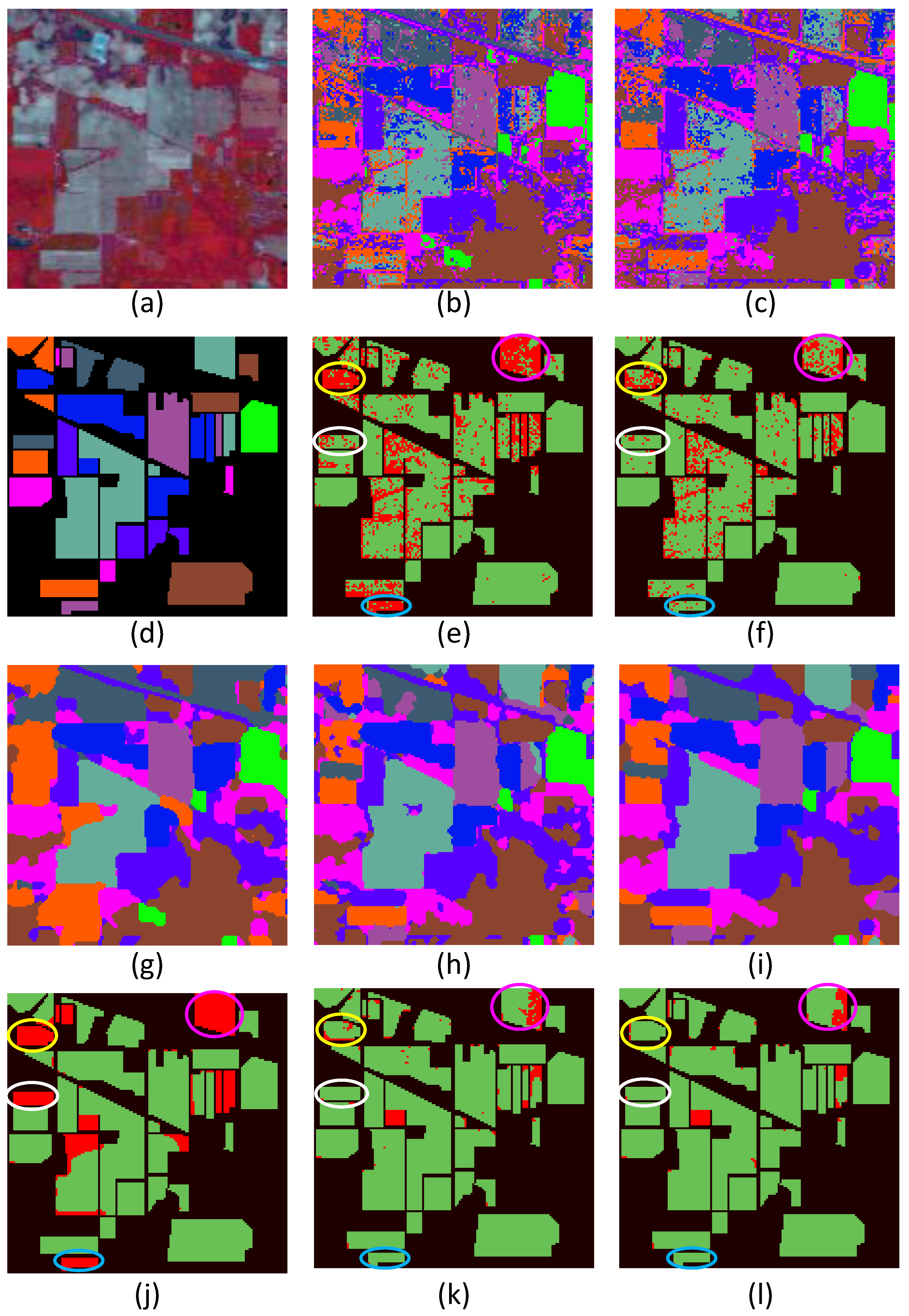
Figure 1 and Figure 2 show experimental results on the Indian Pines and Pavia University datasets. The results were obtained with the tuned parameter values mentioned above. From the classification maps and difference images, we can see that the results of MLR and SVM have abundant salt-and-pepper classification noise. The result of SVM is better than that of MLR, which is consistent with the conclusion in the literature that SVM has robust performance in conditions of high feature dimension and limited training samples, while the MLR has limited generalization ability when training samples are not sufficient [26]. CRFs, SVRFMC, and HSVRFs exhibit better visualization results in that the salt-and-pepper noise is greatly reduced and smoother results are obtained. This is because the spatial context is considered in the four models. However, there is an obvious over-smoothing effect in the classification maps of CRFs, which is illustrated more clearly in the corresponding difference images. In the difference image of CRFs on Indian Pines (Figure 1j), it is clear that there are patches which are entirely misclassified (shown in circles in Figure 1j). For example, on comparing the classification map and difference image of CRFs (Figure 1g,j), we can see that the corn-notill patch (shown in the yellow circle) in the top-left corner is misclassified into corn-mintill. The soybean-mintill patch (shown in the purple circle) in the top-right is misclassified into soybean-clean. Meanwhile, the soybean-clean patch (shown in the white circle) in the left of the image is misclassified into corn-mintill, and the soybean-notill patch (shown in the blue circle) at the bottom of the image is misclassified into soybean-mintill. In contrast, the results of SVRFMC and HSVRFs are much better. For example, from the difference images of SVRFMC and HSVRFs on the Indian Pines image (Figure 1k,l), we can see that the four aforementioned misclassified patches in the difference image of CRFs (Figure 1j) are classified correctly in general. This demonstrates the advantage of SVM over MLR used as the unary potential in the CRF framework.

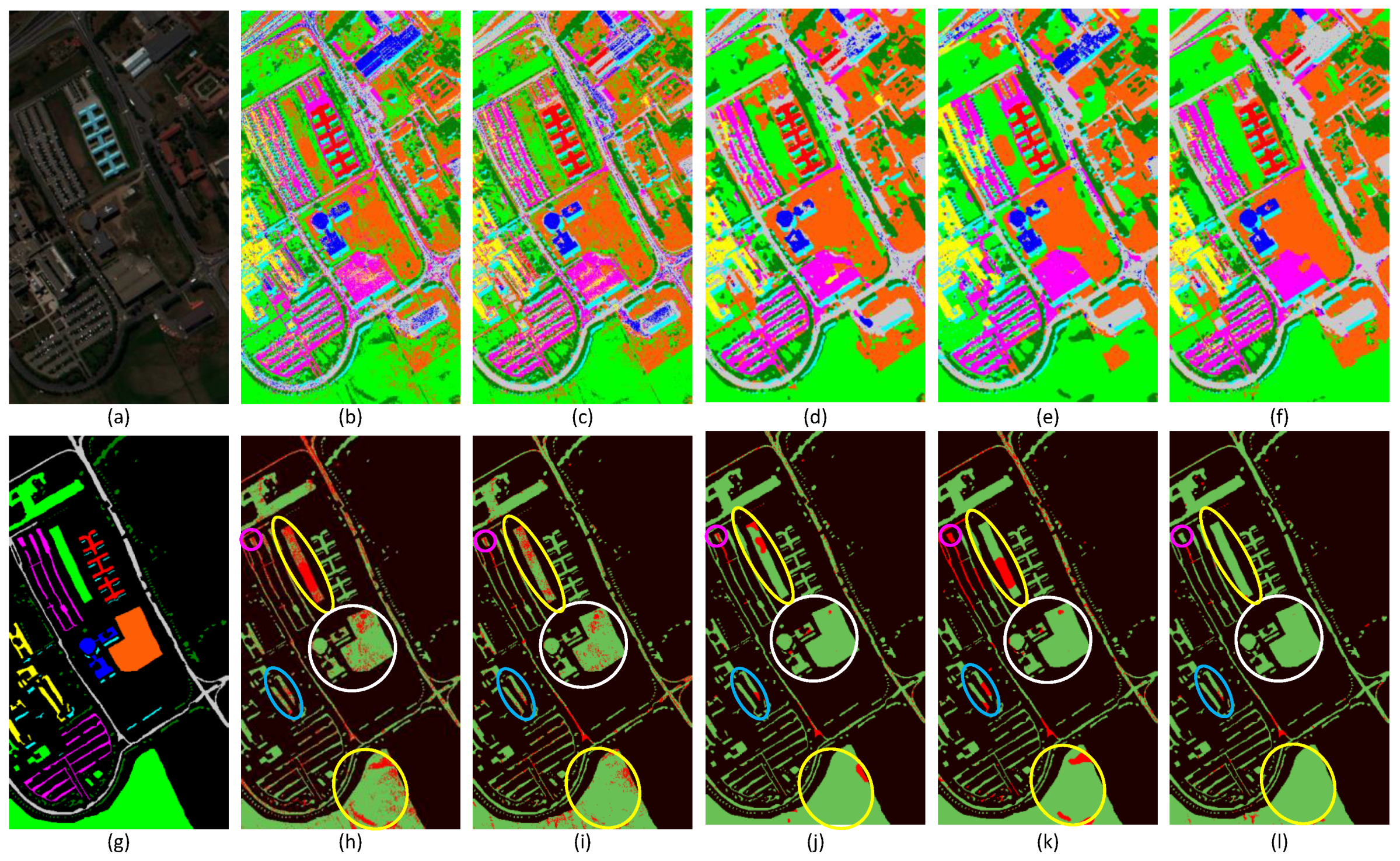
Furthermore, it can be seen that compared to SVRFMC, the HSVRFs model obtains better classification maps. Note that there are still misclassified pixels in the yellow-circled region in the difference image of SVRFMC on the Indian Pines dataset. However, those pixels are correctly classified in the results of HSVRFs. It is worth noting that for the Pavia University dataset, the advantage of the HSVRFs model is more obvious. For example, when comparing the difference images of SVRFMC and HSVRFs for Pavia University, we can see that the misclassified pixels of the Meadow patches (shown in yellow circles), Bitumen patches, Bare Soil patches (shown in white circles), and the Brick patches (shown in purple circles) in the result of the SVRFMC (Figure 2k) are classified into the right classes in the results of the HSVRFs (Figure 2l). The reason for this is that the integration of higher order potentials makes the HSVRFs model capable of modeling high-level contextual information, and thus it can better depict the complicated details in HSI, especially for urban images that contain many complex structures. To conclude, compared to the other four methods, the HSVRFs model can achieve competitive classification maps, showing appropriate smoothing and preserving good boundary information. This can be demonstrated more clearly in the comparison of circled regions in the difference images of the five methods.

To give the quantitative evaluation, Table 1 and Table 2 present class-specific accuracies (percentage of pixels correctly classified for each class), overall accuracy (OA; percentage of pixels correctly classified) and Kappa [51] of compared methods in the two groups of experiments on Indian Pines dataset. Table 3 shows the accuracies of compared methods on the Pavia University dataset. We ran each experiment five times with different randomly chosen training/testing sets and reported the mean classification accuracies.

In the first group of experiments on the Indian Pines dataset, HSVRFs obtained the highest OA and Kappa at 94.83% and 93.81% respectively, which were 1.36% and 1.61% higher than the corresponding values for SVRFMC, and these were the highest class-specific accuracies for most classes. The OA of SVM was 85.52%, which was about 8.9% higher than that of MLR. The OA of SVRFMC was about 6.44% higher than that of CRFs, which demonstrates the advantage of SVM over MLR working as the unary classifier in CRFs framework. In the second group of experiments on this dataset, HSVRFs also acquired the highest OA at 98.50%, which was 1.07% and 4.81% higher than the corresponding of the SVRFMC and CRF-H [27], respectively. It is notable that even with the higher order potential, the OA of CRF-H is still lower than that of SVRFMC. The reason for this phenomenon can be ascribed to the advantage of SVM in SVRFMC over the MLR in CRF-H, and also the advantage of the Mahalanobis distance boundary constraint in SVRFMC over the Ising model in CRF-H.

In the Pavia University dataset with more complex structures, the HSVRFs obtained the highest OA and Kappa at 96.67% and 97.10% respectively. These values were 2.02% and 3.98% higher than the corresponding values for the SVRFMC. The OA of SVRFMC was 6.23% higher than that of CRFs. Over the two datasets, the OAs of CRFs, CRF-H, SVRFMC, and HSVRFs were higher than those of non-contextual MLR and SVM, which shows the importance of contextual information. The HSVRFs achieved the best performance among all the six methods. Furthermore, the advantage of HSVRFs over SVRFMC on the Pavia University dataset is more obvious than that on the Indian Pines dataset. This validates the suitability of the proposed higher order potentials for modeling urban HSI containing more complex structures.

3.3. Parameter Analysis

In the proposed HSVRFs model, there are three main factors that have an influence on the final classification accuracy. The first is the threshold parameter T which controls the rigidity of the higher order potentials, the second is the number of superpixels (i.e., segments) in the ER over-segmentation algorithm, and the third is the number of training samples. In this section, we give the analysis about classification performance of the model with various values of the three parameters.

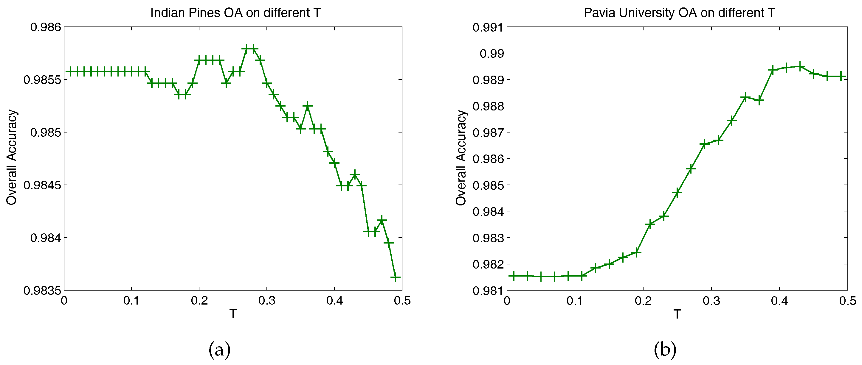
Figure 3 gives the OA curves of the HSVRFs model in relation to different values of T. Each OA reported in the curves was the average value of five experiments with different randomly chosen training sets. The other parameters were kept the same as those mentioned in Section 3.1. For the two datasets, we tuned the values of T from 0.01 to 0.49, with a stepsize of 0.01. From the two curves, we can see that the highest OA was obtained when $T=0.27$ for the Indian Pines dataset, and $T=0.43$ for Pavia University. This was reported in the selected parameter values in Section 3.1.

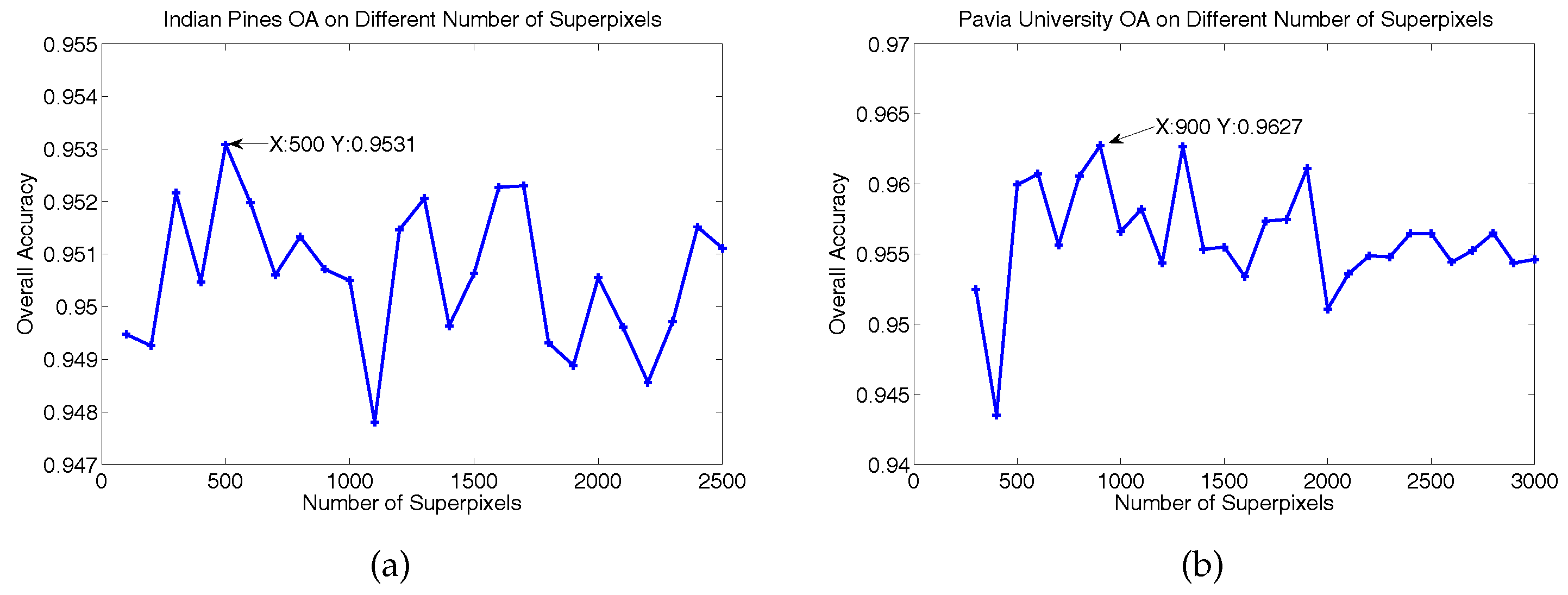
Figure 4 gives the OA curves of the HSVRFs model in relation to different number of superpixels in ER algorithm. Each OA reported in the curves was also the average value of five experiments with different randomly chosen training sets. The other parameters were set the same as those mentioned in Section 3.1. For the Indian Pines dataset, we tuned the number of superpixels from 100 to 2500, with a stepsize of 100. For the Pavia University dataset, we tuned the number of superpixels from 300 to 3000, with a stepsize of 100. From the two curves, we can see that the highest OA was obtained when the number of superpixels was 500 for Indian Pines dataset, and 900 for Pavia University.

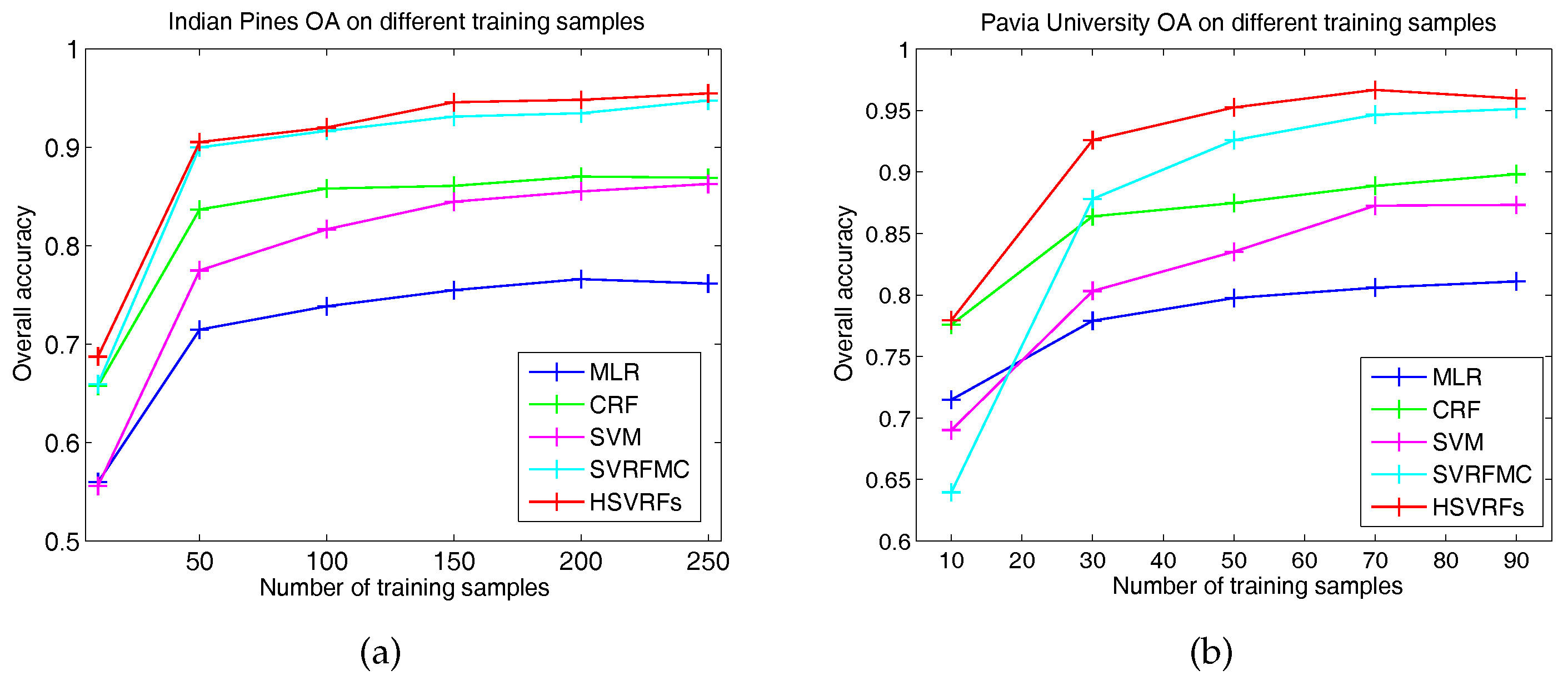
Figure 5 gives the OA curves of MLR, CRF, SVM, SVRFMC, and HSVRFs in relation to different numbers of training samples. Each OA reported the 5-time average overall accuracy. All the other parameters were set the same as those mentioned in Section 3.1. For the Indian Pines dataset, the number of training samples varied from 10 to 250, with a stepsize of 50 except for the first and second point in the curves. For the Pavia University dataset, the number of training samples varied from 10 to 90, with a stepsize of 20. We note that on the two datasets, the OAs of the compared methods grew with the increase in training samples, but the growth became slower when the numbers of training samples increased to a certain point. The HSVRFs model performed the best among the five methods on the two datasets. Lastly, the HSVRFs model obtained the highest OA when the number of training samples was 200 for the Indian Pines dataset and 70 for the Pavia University dataset, which was reported in Section 3.1.

4. Conclusions

In this work, we propose a novel CRF model named HSVRFs for HSI classification. By incorporating higher order potentials into the SVRFMC model, the HSVRFs model not only takes advantage of the SVM classifier and Mahalanobis distance boundary constraint in the SVRFMC model, but can also capture higher-level contextual information. Moreover, we weight the pixels in each segment, on which the higher order potentials are defined, with their label confidences given by the SVM classifier in our framework. This weighting strategy further enhances the depiction ability of the higher order potentials in our model. Experiments on two real HSI datasets show that the HSVRFs model has better performance than the traditional MLR, SVM, and CRFs methods, and also outperforms the recently proposed SVRFMC and CRF-H models. The experiments also reveal that the HSVRFs model is especially efficient for HSI in urban areas, as it has high spatial resolution and contains complicated structures and boundaries.

Currently, the pairwise potentials in our HSVRFs model are defined on neighboring pixels in the 8-neighborhood. A further step is to define the pairwise potentials on neighboring superpixels (superpixels sharing edges), which will incorporate a longer-range spatial context that may further improve the classification result. This is part of our future work to better explore the spatial contextual information in HSI. Moreover, the integration of higher order potentials in HSVRFs brings additional computations on feature value calculation and model inference. Thus HSVRFs cost more computational time compared to second-order CRF frameworks. Moreover, we also hope to investigate the efficiency improvement of this model in our future work.

References

- Hughes, G. On the mean accuracy of statistical pattern recognizers. IEEE Trans. Inf. Theory 1968, 14, 55–63. [Google Scholar] [CrossRef]
- Vapnik, V.N. Statistical Learning Theory; Wiley: Hoboken, NJ, USA, 1998. [Google Scholar]
- Gualtieri, J.; Chettri, S. Support vector machines for classification of hyperspectral data. In Proceedings of the IEEE 2000 International Geoscience and Remote Sensing Symposium (IGARSS 2000), Honolulu, HI, USA, 24–28 July 2000; Volume 2, pp. 813–815. [Google Scholar]
- Melgani, F.; Bruzzone, L. Classification of hyperspectral remote sensing images with support vector machines. IEEE Trans. Geosci. Remote Sens. 2004, 42, 1778–1790. [Google Scholar] [CrossRef]
- Camps-Valls, G.; Gomez-Chova, L.; Munoz-Mari, J.; Vila-Frances, J.; Calpe-Maravilla, J. Composite kernels for hyperspectral image classification. IEEE Geosci. Remote Sens. Lett. 2006, 3, 93–97. [Google Scholar] [CrossRef]
- Tarabalka, Y.; Benediktsson, J.A.; Chanussot, J. Spectral-spatial Classification of Hyperspectral Imagery Based on Partitional Clustering Techniques. IEEE Trans. Geosci. Remote Sens. 2009, 47, 2973–2987. [Google Scholar] [CrossRef]
- Khodadadzadeh, M.; Li, J.; Plaza, A.; Ghassemian, H.; Bioucas-Dias, J.M. Spectral-spatial classification for hyperspectral data using SVM and subspace MLR. In Proceedings of the 2013 IEEE International Geoscience and Remote Sensing Symposium (IGARSS), Melbourne, VIC, Australia, 21–26 July 2013; pp. 2180–2183. [Google Scholar]
- Campsvalls, G.; Tuia, D.; Bruzzone, L.; Atli Benediktsson, J. Advances in Hyperspectral Image Classification: Earth Monitoring with Statistical Learning Methods. IEEE Signal Process. Mag. 2014, 31, 45–54. [Google Scholar] [CrossRef]
- Zhong, P.; Wang, R. Learning conditional random fields for classification of hyperspectral images. IEEE Trans. Image Process. 2010, 19, 1890–1907. [Google Scholar] [CrossRef] [PubMed]
- Zhong, Y.; Zhao, J.; Zhang, L. A hybrid object-oriented conditional random field classification framework for high spatial resolution remote sensing imagery. IEEE Trans. Geosci. Remote Sens. 2014, 52, 7023–7037. [Google Scholar] [CrossRef]
- Lafferty, J.; McCallum, A.; Pereira, F.C. Conditional Random Fields: Probabilistic Models For Segmenting And Labeling Sequence Data. Proceeding of the Eighteenth International Conference on Machine Learning (ICML ’01), San Francisco, CA, USA, 28 June–1 July 2001; pp. 282–289. [Google Scholar]
- Kumar, S.; Hebert. Discriminative Random Fields: A Discriminative Framework for Contextual Interaction in Classification. Proceeding of the Ninth IEEE International Conference on Computer Vision, Nice, France, 13–16 October 2003; IEEE Computer Society: Washington, DC, USA, 2003; pp. 1150–1157. [Google Scholar]
- Shotton, J.; Winn, J.; Rother, C.; Criminisi, A. TextonBoost: Joint Appearance, Shape and Context Modeling for Multi-class Object Recognition and Segmentation. Proceeding of the Computer Vision ECCV 2006, Graz, Austria, 7–13 May 2006; Springer: Berlin/Heidelberg, Germany, 2006; pp. 1–15. [Google Scholar]
- Shotton, J.; Winn, J.; Rother, C.; Criminisi, A. Textonboost for image understanding: Multi-class object recognition and segmentation by jointly modeling texture, layout, and context. Int. J. Comput. Vis. 2009, 81, 2–23. [Google Scholar] [CrossRef]
- He, X.; Zemel, R.S.; Carreira-Perpiñán, M.Á. Multiscale conditional random fields for image labeling. Proceeding of the IEEE Computer Vision and Pattern Recognition, Washington, DC, USA, 27 June–2 July 2004; pp. 695–702. [Google Scholar]
- He, X. Learning Structured Prediction Models for Image Labeling; University of Toronto: Toronto, ON, Canada, 2008. [Google Scholar]
- Torralba, A.; Murphy, K.P.; FFreeman, W.T. Contextual models for object detection using boosted random fields. In Proceedings of the Advances in Neural Information Processing Systems, Vancouver, BC, Canada, 13–18 December 2004. [Google Scholar]
- Gould, S.; Rodgers, J.; Gould, S.; Rodgers, J.; Cohen, D.; Elidan, G.; Koller, D. Multi-class segmentation with relative location prior. Int. J. Comput. Vis. 2008, 80, 300–316. [Google Scholar] [CrossRef]
- Gould, S.; Fulton, R.; Koller, D. Decomposing a scene into geometric and semantically consistent regions. Proceeding of the 2009 IEEE 12th International Conference on Computer Vision, Kyoto, Japan, 29 September–2 October 2009; pp. 1–8. [Google Scholar]
- Ladicky, L.; Sturgess, P.; Russell, C.; Sengupta, S.; Bastanlar, Y.; Clocksin, W.; Torr, P.H. Joint optimization for object class segmentation and dense stereo reconstruction. Int. J. Comput. Vis. 2012, 100, 122–133. [Google Scholar] [CrossRef]
- Ladicky, L.; Russell, C.; Kohli, P.; Torr, P.H. Associative hierarchical CRF for object class image segmentation. Proceeding of the 2009 IEEE 12th International Conference on Computer Vision, Kyoto, Japan, 29 September–2 October 2009; pp. 739–746. [Google Scholar]
- Huang, Q.; Han, M.; Wu, B.; Ioffe, S. A hierarchical conditional random field model for labeling and segmenting images of street scenes. Proceeding of the IEEE Conference on Computer Vision and Pattern Recognition, Colorado Springs, CO, USA, 20–25 June 2011; pp. 1953–1960. [Google Scholar]
- Li, X.; Sahbi, H. Superpixel-Based Object Class Segmentation Using Conditional Random Fields. Proceeding of the 36th IEEE International Conference on Acoustics, Speech, and Signal Processing (ICASSP 2011), Prague, Czech Republic, 22–27 May 2011; pp. 1101–1104. [Google Scholar]
- Kohli, P.; Ladicky, L.; Torr, P.H.S. Robust higher order potentials for enforcing label consistency. Int. J. Comput. Vis. 2009, 82, 302–324. [Google Scholar] [CrossRef]
- Kohli, P.; Kumar, M.P.; Torr, P.H.S. P3 and beyond: Solving energies with higher order cliques. Proceeding of the IEEE Conference on Computer Vision and Pattern Recognition, Minneapolis, MN, USA, 17–22 June 2007; pp. 1–8. [Google Scholar]
- Zhong, Y.; Lin, X.; Zhang, L. A support vector conditional random fields classifier with a mahalanobis distance boundary constraint for high spatial resolution remote sensing imagery. IEEE J. Sel. Top. Appl. Earth Obs. Remote Sens. 2014, 7, 1314–1330. [Google Scholar] [CrossRef]
- Zhong, P.; Wang, R. Modeling and classifying hyperspectral imagery by CRFs with sparse higher order potentials. IEEE Trans. Geosci. Remote Sens. 2011, 49, 688–705. [Google Scholar] [CrossRef]
- Zhong, P.; Liu, F.; Wang, R. Learning sparse conditional random fields to select features for land development classification. Int. J. Remote Sens. 2011, 32, 4203–4219. [Google Scholar] [CrossRef]
- Zhong, P.; Wang, R. Jointly learning the hybrid CRF and MLR model for simultaneous denoising and classification of hyperspectral imagery. IEEE Trans. Neural Netw. Learn. Syst. 2014, 25, 1319–1334. [Google Scholar] [CrossRef]
- Zhao, J.; Zhong, Y.; Zhang, L. Detail-Preserving Smoothing Classifier Based on Conditional Random Fields for High Spatial Resolution Remote Sensing Imagery. IEEE Trans. Geosci. Remote Sens. 2015, 53, 2440–2452. [Google Scholar] [CrossRef]
- Besbes, O.; Benazza-Benyahia, A. Road network extraction by a higher-order CRF model built on centerline cliques. Proceeding of the IEEE 23rd European Signal Processing Conference, Nice, France, 31 August–4 September 2015; pp. 1631–1635. [Google Scholar]
- Li, E.; Femiani, J.; Xu, S.; Zhang, X.; Wonka, P. Robust Rooftop Extraction From Visible Band Images Using Higher Order CRF. IEEE Trans. Geosci. Remote Sens. 2015, 53, 4483–4495. [Google Scholar] [CrossRef]
- Aghighi, H.; Trinder, J.; Tarabalka, Y.; Lim, S. Dynamic Block-Based Parameter Estimation for MRF Classification of High-Resolution Images. IEEE Geosci. Remote Sens. Lett. 2014, 11, 1687–1691. [Google Scholar] [CrossRef]
- Tarabalka, Y.; Rana, A. Graph-Cut-Based Model for Spectral-Spatial Classification of Hyperspectral Images. Proceeding of the 2014 IEEE International Conference on Geoscience and Remote Sensing Symposium (IGARSS), Quebec City, QC, Canada, 13–18 July 2014; pp. 3418–3421. [Google Scholar]
- Lee, C.H.; Greiner, R.; Schmidt, M. Support vector random fields for spatial classification. In Knowledge Discovery in Databases: PKDD 2005; Springer: New York, NY, USA, 2005; pp. 121–132. [Google Scholar]
- Zhang, G.; Jia, X. Simplified Conditional Random Fields With Class Boundary Constraint for Spectral-Spatial Based Remote Sensing Image Classification. IEEE Geosci. Remote Sens. Lett. 2012, 9, 856–860. [Google Scholar] [CrossRef]
- Cheng, Q.; Varshney, P.K.; Arora, M.K. Logistic regression for feature selection and soft classification of remote sensing data. IEEE Geosci. Remote Sens. Lett. 2006, 3, 491–494. [Google Scholar] [CrossRef]
- Platt, J. Probabilistic Outputs for Support Vector Machines and Comparisons to Regularized Likelihood Methods. Adv. Large Margin Classif. 1999, 10, 61–74. [Google Scholar]
- Liu, M.Y.; Tuzel, O.; Ramalingam, S.; Chellappa, R. Entropy rate superpixel segmentation. Proceeding of the 2011 IEEE Conference on Computer Vision and Pattern Recognition (CVPR), Colorado Springs, CO, USA, 20–25 June 2011; pp. 2097–2104. [Google Scholar]
- Waske, B.; Benediktsson, J.A. Fusion of support vector machines for classification of multisensor data. IEEE Trans. Geosci. Remote Sens. 2007, 45, 3858–3866. [Google Scholar] [CrossRef]
- Huang, C.; Davis, L.S.; Townshend, J.R.G. An assessment of support vector machines for land cover classification. Int. J. Remote Sens. 2002, 23, 725–749. [Google Scholar] [CrossRef]
- Wu, T.F.; Lin, C.J.; Weng, R.C. Probability estimates for multi-class classification by pairwise coupling. J. Mach. Learn. Res. 2004, 5, 975–1005. [Google Scholar]
- Chang, C.C.; Lin, C.J. LIBSVM: A library for support vector machines. ACM Trans. Intell. Syst. Technol. (TIST) 2011, 2, 27. [Google Scholar] [CrossRef]
- Sutton, C.; McCallum, A. Piecewise pseudolikelihood for efficient training of conditional random fields. In Proceedings of the 24th International Conference on Machine Learning, Corvalis, OR, USA, 20–24 June 2007; ACM: New York, NY, USA, 2007; pp. 863–870. [Google Scholar]
- Besag, J. Statistical analysis of non-lattice data. Statistician 1975, 24, 179–195. [Google Scholar] [CrossRef]
- Boykov, Y.; Veksler, O.; Zabih, R. Fast approximate energy minimization via graph cuts. IEEE Trans. Pattern Anal. Mach. Intell. 2001, 23, 1222–1239. [Google Scholar] [CrossRef]
- Aviris, N. Indiana’s Indian Pines 1992 Data Set. 2012. Available online: http://www.ehu.eus/ccwintco/index.php?title=HyperspectralRemoteSensingScenes (accessed on 24 October 2017).
- Zhong, P.; Wang, R. Learning sparse CRFs for feature selection and classification of hyperspectral imagery. IEEE Trans. Geosci. Remote Sens. 2008, 46, 4186–4197. [Google Scholar] [CrossRef]
- Rumelhart, D.E.; Hinton, G.E.; Williams, R.J. Learning representations by back-propagating errors. Cognit. Model. 1988, 5, 3. [Google Scholar] [CrossRef]
- Bryson, A.E. Applied Optimal Control: Optimization, Estimation and Control; Halsted Press: Sydney, Australia, 1975. [Google Scholar]
- Arora, H.; Loeff, N.; Forsyth, D.; Ahuja, N. Unsupervised segmentation of objects using efficient learning. Proceeding of the IEEE Conference on Computer Vision and Pattern Recognition (CVPR’07), Minneapolis, MN, USA, 17–22 June 2007; pp. 1–7. [Google Scholar]
Figure 1.
Classification results of the Indian Pines dataset (with 200 training samples for each class). (a) Three-band false color image. (d) Ground truth. (b,c,g–i) Classification maps obtained by multinomial logistic regression (MLR), support vector machines (SVMs), conditional random fields (CRFs), support vector random fields with a Mahalanobis distance boundary constraint (SVRFMC), and higher order support vector random fields (HSVRFs). (e,f,j–l) The corresponding difference images of (b,c,g–i) compared with the ground truth in (d). Black regions represent pixels without ground truth; In the rest of the areas, green regions represent correctly classified pixels and red regions represent wrongly classified pixels.
Figure 2.
Classification results of Pavia University dataset. (a) Three-band false color image. (g) Ground truth. (g,f) Classification maps obtained by MLR, SVMs, CRFs, SVRFMC, and HSVRFs. (h–l) The corresponding difference images of (b–f) compared with the ground truth in (g). Black regions represent pixels without ground truth. In the remaining part, green regions represent correctly classified pixels and red regions represent wrongly classified pixels.
Figure 3.
Overall classification accuracies for different values of T. (a,b) show the OA versus different values of T on the Indian Pines and Pavia University datasets, respectively.
Figure 4.
Overall classification accuracies for different numbers of superpixels. (a,b) show the OA versus different numbers of superpixels on the Indian Pines and Pavia University datasets, respectively.
Figure 5.
Overall classification accuracies with different numbers of training samples. (a,b) show the OA versus different numbers of training samples on the Indian Pines and Pavia University datasets, respectively.