Article

Urban Growth Modeling and Future Scenario Projection Using Cellular Automata (CA) Models and the R Package Optimx

1
College of Marine Sciences & National Distant-Water Fisheries Engineering Research Center, Shanghai Ocean University, Shanghai 201306, China
2
School of Earth and Environmental Sciences, University of Queensland, Brisbane, QLD 4072, Australia
3
College of Surveying and Geo-Informatics, Tongji University, Shanghai 200092, China
*
Authors to whom correspondence should be addressed.
ISPRS Int. J. Geo-Inf. 2018, 7(10), 387; https://0-doi-org.brum.beds.ac.uk/10.3390/ijgi7100387
Submission received: 30 July 2018 / Revised: 25 August 2018 / Accepted: 22 September 2018 / Published: 25 September 2018
(This article belongs to the Special Issue Urban Environment Mapping Using GIS)

Abstract

:
Cellular automata (CA) is a spatially explicit modeling tool that has been shown to be effective in simulating urban growth dynamics and in projecting future scenarios across scales. At the core of urban CA models are transition rules that define land transformation from non-urban to urban. Our objective is to compare the urban growth simulation and prediction abilities of different metaheuristics included in the R package optimx. We applied five metaheuristics in optimx to near-optimally parameterize CA transition rules and construct CA models for urban simulation. One advantage of metaheuristics is their ability to optimize complexly constrained computational problems, yielding objective parameterization with strong predictive power. From these five models, we selected conjugate gradient-based CA (CG-CA) and spectral projected gradient-based CA (SPG-CA) to simulate the 2005–2015 urban growth and to project future scenarios to 2035 with four strategies for Su-Xi-Chang Agglomeration in China. The two CA models produced about 86% overall accuracy with standard Kappa coefficient above 69%, indicating their good ability to capture urban growth dynamics. Four alternative scenarios out to the year 2035 were constructed considering the overall effect of all candidate influencing factors and the enhanced effects of county centers, road networks and population density. These scenarios can provide insight into future urban patterns resulting from today’s urban planning and infrastructure, and can inform future development strategies for sustainable cities. Our proposed metaheuristic CA models are also applicable in modeling land-use and urban growth in other rapidly developing areas.

1. Introduction

Spatial explicit modeling (SEM) has been effective and increasingly applied in studies of land-use change [1,2], particularly in rapidly urbanizing areas like China’s coastal zones. Among the SEM methods, cellular automata (CA) has become the most widely used approach to first reproduce past landscape and urban patterns and then predict future scenarios under specific development strategies [3,4,5,6]. CA models have provided a basis for rational urban spatial expansion that could reduce conflicts between land exploitation and conservation [7]. A gridded CA model divides space into equally-sized and uniformly-distributed cells [8], and then defines non-urban to urban cell conversion rules [9]. The transformation potential of each cell is usually reflected by the probability calculated based on urban growth drivers [10,11]. The transition rules can be parameterized using approaches that range from conventional statistical techniques to state-of-the-art artificial intelligence algorithms [12]. While many specific methods have been integrated with CA modeling, it is necessary to compare models with a unified framework.
Attempts over the past two decades to build and optimize CA transition rules have led to smaller departures between simulation results and reference patterns and more defensible future scenarios [3,4,13,14]. Among the techniques that have been tested, logistic regression (LR) is the most widely acknowledged and applied statistical method used to capture CA transition rules [3]. More recently, artificial intelligence and machine learning methods have increasingly been applied in creating new CA models [4].
Metaheuristics are partial-search artificial intelligence algorithms that are capable of minimizing residuals when defining near-optimal CA parameters [15,16], ultimately achieving more accurate simulations. For CA model calibration, metaheuristics are superior because they incorporate complex real-world constraints in the optimization procedure through mathematically expressed equalities and/or inequalities [17], allowing metaheuristics to search for alternative CA parameters in future scenario prediction.
Many (intelligent) metaheuristics have recently been used to calibrate hybrid CA models of land-use change and urban growth [18], e.g., genetic algorithm (GA), particle swarm optimization (PSO), simulated annealing (SA), generalized pattern search (GPS), ant colony optimization (ACO), bat movement algorithm (BA), differential evolution (DE), artificial bee colony (ABC), and Cuckoo search (CS) [19,20,21,22,23]. These algorithms originated in simulating natural phenomena corresponding to complex optimization [20,24,25]. They guide the optimization using a fitness function, which is typically built on the deviations (residuals) between the actual classifications and the simulation results [17]. Each metaheuristic has a different internal scheme to guide optimization [26], and most metaheuristics do not require differentiation of the fitness function. For urban CA modeling, the fitness function that evaluates the residuals and/or the fitness of the transition rules is discrete and non-derivable [20,23]. Therefore, the derivative-free metaheuristics are ideal for building the CA transition rules.
CA transition rules have commonly been presented in three forms: (1) “if-then” and/or “what-if” rules that denote cell state transformation from non-urban to urban if one of the transition rules is met [23,27,28], (2) factor-weighted transition rules that calculate the probability of each non-urban cell transforming to an urban cell [17,20], and (3) black-box transition rules that do not clearly show the cell transformation procedure [24,29]. Artificial neural networks (ANNs) generate transition rules using black-box methods; metaheuristics such as ACO and CS create the transition rules through “if-then”/“what-if” rules; SA, GPS, PSO, GA, DE, BA, and ABC express transition rules with mathematical formulae similar to those derived from LR. GA can define the transition rules using both transition rule styles [20,30].
Previous work has demonstrated that these metaheuristics can be effective in exploring optimized CA parameters that adequately address land-use and urban growth dynamics [19,20,21,25,29]. Metaheuristic codes and scripts are widely available in C++, Matlab, Python and R, facilitating their application in urban CA modeling. Some open-source R packages contain different versions of most metaheuristics that are readily applicable to the retrieval of CA transition rules. Among these R packages, optimx unifies and streamlines optimization in solving many functions [31,32]. Compared to other packages, optimx consolidates existing metaheuristics to facilitate the comparative study of urban CA modeling.
Our objective is to compare the urban growth simulation and prediction abilities of different metaheuristics included in the R packages optimx. We selected five optimx metaheuristics to build CA models that simulate the urban growth during 2005–2015 in the Su-Xi-Chang (Suzhou, Wuxi and Changzhou) Agglomeration of China, and to predict alternative scenarios under different inequalities representing various urban development strategies. This research could enrich the urban CA modeling techniques by applying new heuristic algorithms, and improve our understanding of urban dynamics.

2. Methods

2.1. A Prototype CA Model and the Fitness Function

Urban CA models focus on urban expansion simulation that can be realized by land transition rules. In these models, the probability of non-urban to urban cell transformation is usually defined by an overall probability [4,33] that considers the combined effects of the current state, neighborhood influence, external constraints, and transition probability governed by selected urban growth drivers. The overall probability is compared to a pre-defined threshold to determine if a non-urban cell can transform its state. The decision rule is [17,33]:
S t a t e i , t + 1 = { U r b a n , P ( S t a t e i , t , N H i , C o n , P s v i ) P t h d N o n u r b a n , P ( S t a t e i , t , N H i , C o n , P s v i ) < P t h d
where
S t a t e i , t and S t a t e i , t + 1 indicate the cell’s state i at time steps t and t + 1, respectively. Three states (Urban, Non-urban and Water) are allowed;
P ( S t a t e i , t , N H i , C o n , P s v i ) is the predicted overall land transition probability, taking into account all effects;
Pthd is a pre-defined threshold determining if the cell i can transform its state or not;
NHi denotes the effect of neighboring cells on the central cell in processing;
Con denotes the spatially and non-spatially constrained conditions to cell conversion, e.g., protected land and broad water bodies [10]; and
P s v i ( a ) denotes the predicted land transition probability through analyzing the relationships between urban growth and its driving factors.
The latter probability can be calculated [5,33] by:
P s v i ( a ) = 1 / ( 1 + e ( a 0 + i = 1 k a i V i ) )
where ( V 1 , , V k ) are driving factors and a = ( a 0 , , a k ) are a constant and the estimated weights of the driving factors.
This research estimated the weights using the optimx metaheuristics to calibrate CA models. The metaheuristics were processed based on a fitness function representing the residuals in fitting the relationships between urban growth and its drivers. The fitness function can be given by [17,34]:
{ Minimize   F u n c ( a ) = SquareRoot ( i S u m ( P s v i P o i ) 2 / S u m ) s t 1 : Box   constraints: :   L a j a j U a j ,   j = 0 , , k s t 2 : E q u a l i t i e s   a n d   i n e q u a l i t i e s   f o r   f a c t o r   w e i g h t s
where F u n c ( a ) denotes the fitness function, P s v i denotes the predicted land transition probability for cell i, S u m denotes the number of samples, and L a j and U a j are the lower and upper bounds for the CA parameters, respectively. Metaheuristics automatically search for the near-optimal CA parameters for model calibration while resolving the fitness function. These parameters were used in (1) to define the decision rules.

2.2. Metaheuristics in the R Package Optimx

The R-Gui package optimx is a general-purpose optimization wrapper that unifies thirteen metaheuristic optimization algorithms to resolve constrained fitness functions [31]. These metaheuristics are derived from other packages such as “optim”, “ucminf”, “BB” and “Rcgmin”. They are different from those included in packages such as PSO, GA, SA, ACO, and ABC. Compared to these packages, optimx is an effective tool to discover (dis)advantages of metaheuristics [31]. We selected five metaheuristics to calibrate CA models for simulating urban growth dynamics after a pre-test. These five algorithms include Nelder-Mead, Broyden-Fletcher-Goldfarb-Shanno (BFGS), Nonlinear Minimization in Box Constraints (NLMINB), conjugate gradients (CG) and spectral projected gradient (SPG), and all have been widely applied in urban growth modeling, deforestation simulation, and image processing [35,36,37,38,39], showing their strong abilities to optimize spatial problems.
  • Nelder-Mead, also known as downhill simplex, is a practical, derivative-free global search approach to find the optimum of pre-defined fitness functions [40]. The metaheuristic relies heavily on difference vectors between potential solutions with the positional bias inherent in the simplex, which expands and shrinks to adapt to the present fitness value [40]. Nelder-Mead determines the direction between the best and worst points to find nonstationary optimal points that satisfy the convergence conditions. This optimizer is suitable to resolve non-differential fitness functions that project the CA transition rules into the algorithms.
  • BFGS is a quasi-Newton method for solving unconstrained nonlinear optimization problems [41] such as the minimization of RMSE in CA transition rules. In contrast to the Nelder-Mead’s downhill strategy, BFGS applies hill-climbing optimization technique to search for a stationary point in the fitness function. One merit of BFGS is that it has self-correcting ability and superlinear convergence in optimization problems [42]. BFGS does guarantee the convergence for twice continuously differentiable functions [43], but it yields good performance for non-smooth optimization of fitness functions.
  • NLMINB is a box-constrained Newton method that uses port routines, similar to an adaptive nonlinear least-squares algorithm [44], to solve the problems of minimizing nonlinear functions [45]. The metaheuristic evaluates the gradient of the fitness function to return a possible solution vector as the starting point. The NLMINB optimizer included in R has been demonstrated as suitable to resolve the fitness function in CA transition rules [46].
  • CG is an iterative gradient algorithm that solves optimization problems and partial differential optimization equations with a symmetric, positive-definite matrix [47]. It directly searches for an exact solution with specific iterations smaller than the matrix size. CG does not require matrix storage and therefore converges quickly [48]. We applied this metaheuristic to search the CA parameters by minimizing the RMSE of the transition rules.
  • SPG is an efficient gradient method for solving constrained problems using gradient vectors as a search direction in large-scale optimization. This metaheuristic selects a step length related to the spectrum of the underlying local Hessian in the fitness function [49]. By projecting an arbitrary vector onto the feasible solution set, SPG efficiently optimizes the fitness function. Using gradient vectors is usually more effective as a search direction for large-scale optimization. Modelers need not understand complex linear codes and extra linear algebra when using the SPG algorithm [49].

2.3. Model Assessment Methods

Model assessment (validation) is crucial to urban growth modeling because it reports how well the proposed CA models perform and how well the simulations match the actual urban patterns. The land transition probability maps are commonly assessed using fitting statistics, the relative operating characteristic, and the total operating characteristic [50,51]. The simulation results are usually assessed based on a confusion matrix that is derived from cell-by-cell comparison between observed and simulated urban patterns. We applied six indices: overall accuracy and standard Kappa derived from the confusion matrix, correct rejection, hit, miss, and false alarm calculated from an overlaying map of reference and simulated urban growth patterns [52,53]. Overall accuracy represents the match between the reference and simulated maps in proportion to the total cells [54], indicating the overall performance of the CA models in this research. Kappa is a statistic that measures the inter-rater agreement between the reference and simulated maps, with attention given to the possibility of chance agreement [55]. Correct rejection represents the areas that are persistent non-urban cells in both the reference and simulated maps; hit represents the areas that are urban growth cells in both the reference and simulated maps; miss represents the areas that are urban growth cells in the reference map but persistent non-urban cells in the simulated map; and false alarm represents areas that are persistently non-urban in the reference map but urban growth cells in the simulated map. The sum of miss and false alarm is the total error of the simulation.
We evaluated the spatial structure of alternative scenarios using fifteen landscape metrics related to the area and edge, shape, and aggregation categories [56]. The area and edge metrics represent fundamental properties of urban patches. The specific metrics we selected were percentage of landscape (PLAND), largest patch index (LPI) and total edge (TE). Shape metrics denote the shape and size of the urban patches that reflect the spatial conformity of the future scenarios [57]. We selected the perimeter-area fractal dimension (PAFRAC) from the shape category. Aggregation metrics indicate whether the observed spatial distribution of urban scenarios are clumped or dispersed, showing the level of aggregation and subdivision of urban patches. In the aggregation category, we selected number of patches (NP), patch density (PD), landscape shape index (LSI), clumpiness index (CLUMPY), percentage of like adjacencies (PLADJ), patch cohesion index (COHESION), interspersion and juxtaposition index (IJI), aggregation index (AI), landscape division index (DIVISION), effective mesh size (MESH), and splitting index (SPLIT).

3. Model Application

3.1. Study Area and Datasets
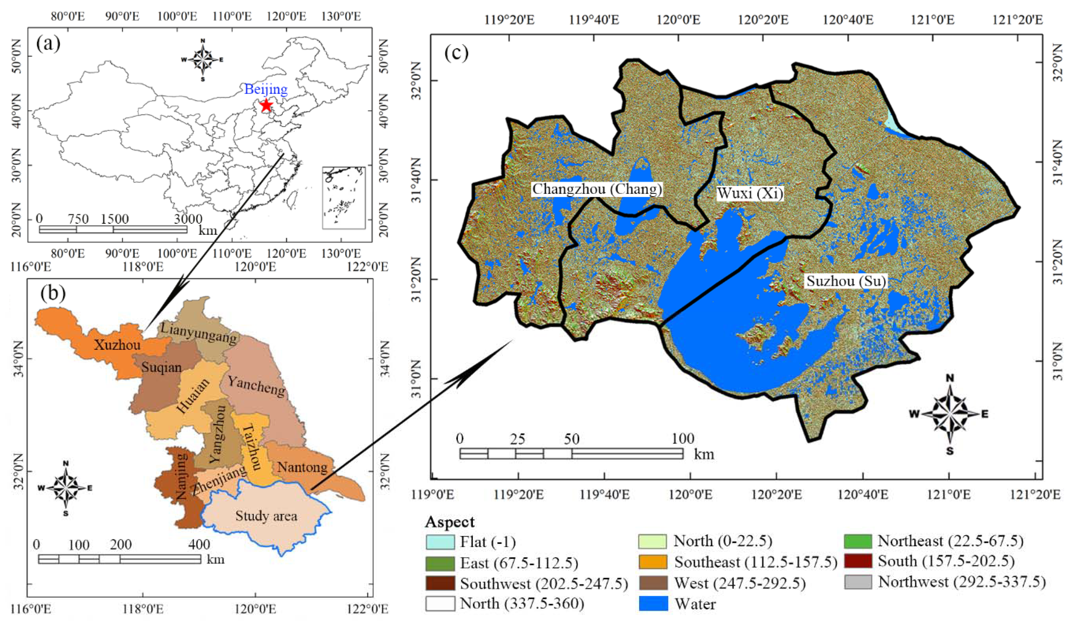
3.1.1. Study Area

The Su-Xi-Chang Agglomeration is a highly urbanized area in southern Jiangsu Province (Figure 1a,b). It consists of three prefecture-level cities (Figure 1c): Suzhou (Su), Wuxi (Xi) and Changzhou (Chang). As the major part of the Taihu Lake Basin, Su-Xi-Chang is a flat area lying below 50 m [58]. The area has a subtropical monsoon climate with warm-humid summer and cold-dry winter. The average annual temperature is about 14–18 °C and the average annual precipitation is about 1000–1400 mm [59]. Su-Xi-Chang is an economically developed area as a consequence of its superior location, convenient transport infrastructure and huge foreign investment. Among all megacities in China, Suzhou, Wuxi and Changzhou ranked the 7th, 13th and 28th in 2015 by GDP. Rapid economic growth and urban development here has been called South-Jiangsu Mode since the 1980s. This growth was accompanied by an urban population explosion and dramatic land-use change in Su-Xi-Chang. Rapid urban growth is a characteristic of China, and Su-Xi-Chang is a representative region that has drawn attention from modelers, planners and decision makers. We chose Su-Xi-Chang as our study area to test the usability, effectiveness and performance of our new CA models.

3.1.2. Factors and Data Sources

Our proposed CA models were calibrated using 2005–2015 urban growth as the dependent variable (Figure 2) and six independent variables (Figure 3). The six independent variables are Distance to city centers (CITY), Distance to county centers (COUNTY), Distances to arterial roads (ROAD), Distances to railway (RAIL), Digital elevation model (DEM), and Population density (POP) (Figure 3), that reflect biophysical and demographic impacts on urban growth. We applied the maximum likelihood classifier in ENVI 5.2 to produce the urban patterns in 2005 and 2015 (Figure 2), using the Landsat images acquired on 7 March 2005 and 13 August 2015, respectively. The overall accuracies of classification were 97.1% for 2005 and 95.9% for 2015, based on comparison between the classified land-use and the identified land-use in the pre-defined regions of interest. Each urban pattern map incorporates three land classes: urban, non-urban, and excluded (broad water bodies and wetlands). The 2005 urban pattern is the start map for modeling while the 2015 urban pattern is the base (reference) for the 2015 simulation. A spatial overlay of these two urban pattern maps was then performed to generate the urban growth map. As inferred by Figure 2, the urban built-up areas increased from 2030 km2 in 1995 to 4779 km2 in 2015, with an annual growth rate of 1.1%.
It should be noted that multicollinearity among factors substantially affects the transition rules and the subsequent urban modeling [60]. We selected the six factors not only because they are the determinants of urban growth in Su-Xi-Chang, but also because they include only the minimum multicollinearity among all candidate factors. Using the ArcGIS 10.1 Euclidean Distance tool, we extracted CITY and COUNTY from the administrative boundary map, and ROAD and RAIL were extracted from the road/rail networks map. Both maps were provided by the National Earth System Science Data Sharing Infrastructure [61], where the road/rail networks map was modified using Google Earth to make it more accurate. These four factors have been shown to be influential and widely applied in urban CA modeling because they reflect the influence of administration and urban facilities [27]. For example, newly built-up areas predominantly occur in urban fringes and along main roads. DEM evaluates land development suitability and was derived from the Geospatial Data Cloud [62]. POP reflects population density and was provided by WorldPop [63], suggesting drivers on urban growth due to the demands of human living space. The spatial resolution of CITY, COUNTY, ROAD, RAIL and DEM was 30 m. POP, with an original resolution of 90 m, was resampled to 30 m using the ArcGIS Bilinear Resampling tool, while keeping the total population as necessary. The bilinear method generated a smooth POP map matching the resolution of other factors. All factors were normalized in the range of [0, 1] to reduce the negative impact of dimensions on retrieval of land transition probability. All maps contain 4724 rows and 6940 columns.

3.2. Results

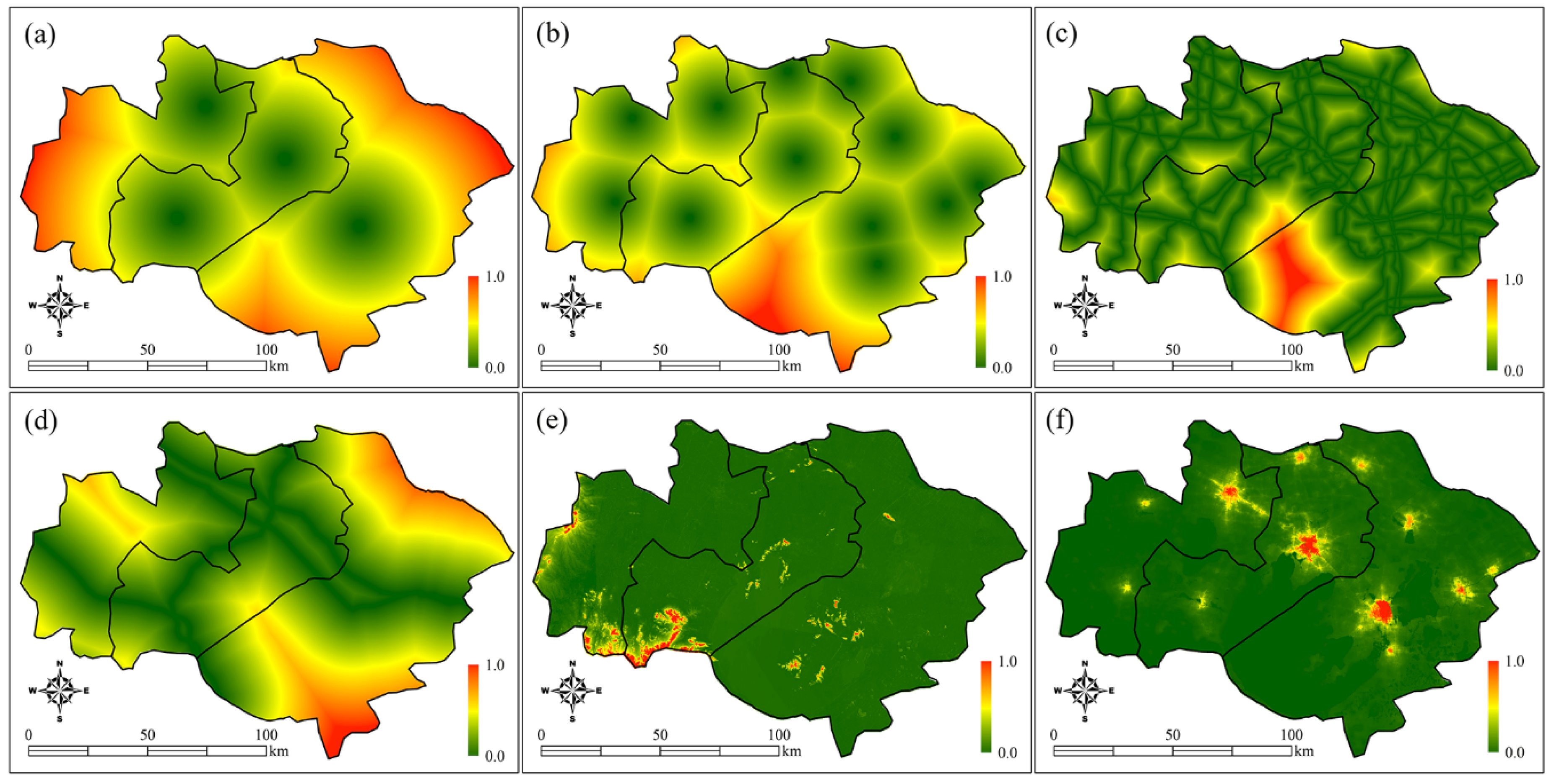
3.2.1. Land Transition Probability Map

Table 1 shows the lower and upper bounds for CA parameters, and the CA parameters retrieved using the five metaheuristics. The CA parameters were the same for Nelder-Mead, BFGS and CG, and are slightly different from those retrieved using NLMINB and SPG. POP is positively correlated with urban growth such that negative POP indicates an impediment to urban growth, possibly because existing built-up areas are densely populated while areas experiencing urban growth are relatively sparsely populated. Except for POP, a greater absolute value of a negative parameter indicates a stronger influence on urban growth, while a greater absolute value of a positive parameter indicates a weaker impact.
These five metaheuristics generated three transition probability maps with similar spatial patterns (Figure 4). Among them, Nelder-Mead and BFGS share the same transition probability map with CG (Figure 4a), because they have the same CA parameters (Table 1). Visual inspection suggests no difference in the probability maps among NLMINB, CG and SPG (Figure 4b,c). However, CG and NLMINB are different—CG yields smaller probability along roads but higher probability in other areas (Figure 4d). The differences between CG and NLMINB are small (−0.0025, 0.0049), suggesting that the two metaheuristics yield quite similar results. In contrast, the difference between CG and SPG and between NLMINB and SPG average about −0.0755, and have a much wider range from −0.28 to 0.24. This suggests that SPG has a higher average value than CG and NLMINB (Figure 4e,f), where the latter are alike.
For scenario prediction, we selected CG from the Nelder-Mead, BFGS and CG metaheuristics that generated similar land transition probability maps. We also selected SPG, which generated a quite different transition probability map. It has been acknowledged that in urban growth modeling a shorter period in calibration can well support a much longer period (e.g., 50 years) of prediction [64,65]. We therefore used the ten-year calibrated CA models to predict four alternative urban scenarios of the next 20 years out to 2035, examining the responses of future scenarios to the pre-defined conditions. These scenarios were (1) a business as usual (BAU) scenario that uses the CA parameters in calibrating CG and SPG (Table 1), (2) a COUNTY-dominated scenario that emphasizes the effects of the county centers (Table 2), (3) a ROAD-dominated scenario that underlines the impacts of the road networks (Table 2), and (4) a POP-dominated scenario that focuses on the influences of population density (Table 2).
Except for the BAU-scenario, all CA parameters of the other three alternative scenarios were retrained using CG and SPG to satisfy prediction requirements. Specifically, the retaining was realized by applying “st2” equalities in Equation (3), where each equality requires that the absolute weight of the dominated factor is larger than those of the other factors. The equalities were defined based on the fact that in the CA transition rules a larger absolute parameter indicates a stronger impact on urban growth. Table 2 shows that the factor emphasized in each scenario yields the most significant impact on urban growth, where there are distinct differences in CA parameters between the two metaheuristics. For the COUNTY-scenario, the COUNTY parameter acquired by CG yields a much higher absolute value (11.3422) compared to that derived by SPG (3.8768), showing the stronger effect of COUNTY in the former metaheuristic. In the ROAD-scenario, the ROAD parameter calculated in CG has a much smaller absolute value (8.6481) as compared with that calculated by SPG (20.101), suggesting weaker impact of ROAD in the former metaheuristic. The absolute POP parameter in the POP-scenario is larger (18.5703) for CG but smaller (4.9698) for SPG, implying higher influence of POP in the former metaheuristic. Because we used the same samples and spatial constraints for model training, it is clear that the differences in factor impact were related to algorithms rather than data.
Using these CA parameters, we produced transition probability maps (Figure 5) for scenario prediction. The maps show differing spatial patterns across factors but similar patterns across metaheuristics. For the COUNTY-scenario, high probability occurred around each satellite city center, with CG yielding high values in smaller areas and SPG yielding high values in larger areas. The spatial patterns generated by POP are somewhat similar to those by COUNTY because the population density in city centers is much higher than that in other areas. For the ROAD-scenario, high probability occurs along the major roads for both CG and SPG, and moderate differences are noticeable between the two metaheuristics. The probability maps clearly reflect the definition of CA parameters and their changes across factors and metaheuristics.

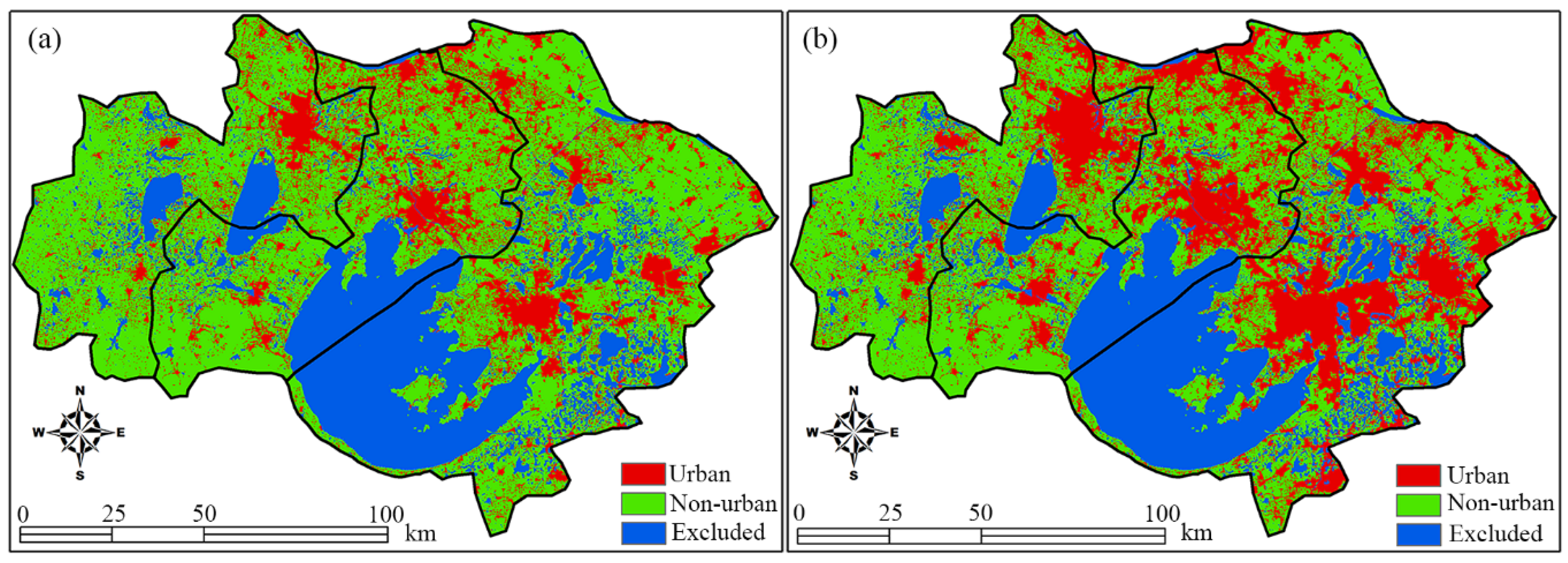
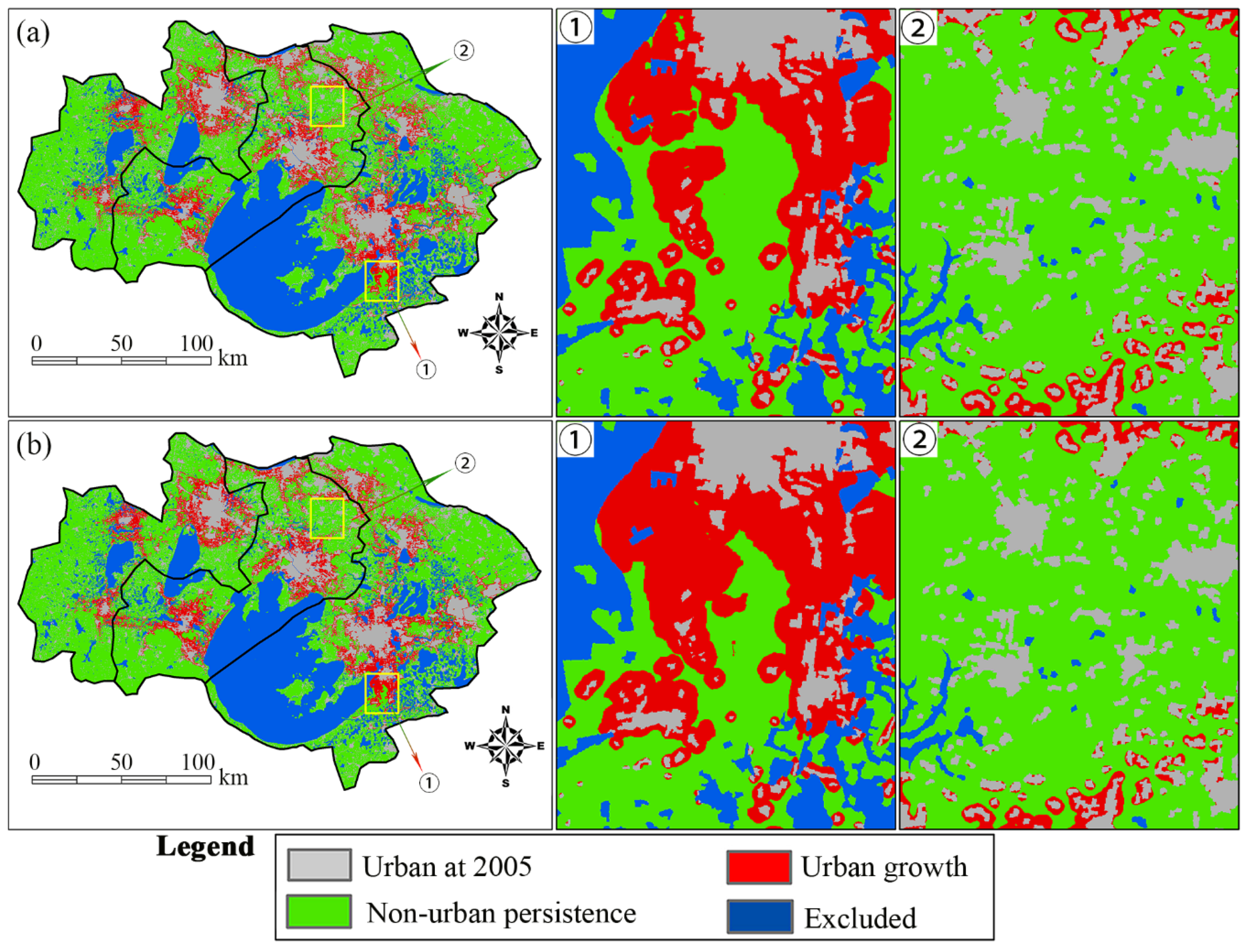
3.2.2. Simulated Urban Patterns for 2015

The transition threshold is critical in determining if a cell’s state can be converted from non-urban to urban state. When the transition probability is larger than the threshold, a non-urban cell will be converted to an urban cell. The optimal threshold was defined using two constraints: (1) the total number of urban cells in 2015, and (2) the maximum running iterations. In this work, there are 5,310,543 urban cells (at 30 m resolution) and the maximum iterations are 10, with each iteration representing one year. CA models are implemented based on a pre-defined probability threshold, and we tested potential thresholds ranging from 0.4 to 0.9 with a 0.1-interval. As the urban cells can only be counted at the end of each iteration of the model implementation, there is always quantitative disagreement between the simulated urban cells and the classified urban cells. Our preliminary experiments show that this disagreement can be possibly controlled to within 1%. As a result, a threshold is appropriate if it results in less than 1% discrepancy in total urban cells at the 10th iteration. In this research, the optimal thresholds we found were 0.56 for CG and 0.70 for SPG.
In comparing the observed urban patterns (see Figure 2), the 2015 simulated urban patterns at Su-Xi-Chang are presented in Figure 6. These were generated using CG-CA and SPG-CA models using the defined thresholds. The maps display similar spatial patterns for urban growth, but they are noticeably different from the observed pattern. Figure 2 shows that the observed newly built-up areas lie in the inner suburbs and the suburban outskirts, while those in the outskirts are dispersed, with many urban patches inserted into the farmland. In contrast, Figure 6 shows that the newly built-up areas are located near the city centers; there are fewer in the outer suburbs, suggesting more compact urban patterns when compared to the observations.
Visual inspection does not show substantial differences between the two simulated maps, so we enlarged two sub-regions in the southeastern and northern urban fringe areas to infer local differences. Region-1 (the middle column) is located in the inner suburbs of Suzhou, where the reference map shows less urban growth while the simulated maps show more urban growth. Substantial differences are apparent between these two enlarged simulated maps. Region-2 (the right column) is located in the outskirts of Wuxi where the reference map shows more urban growth while the simulated maps show less urban growth, with noticeable minor differences between the two enlarged simulation maps. Another significant difference between the reference and simulated maps is that the reference maps are characterized by urban patches with serrated edges, whereas the simulations have urban patches with smooth edges (the middle and right columns).

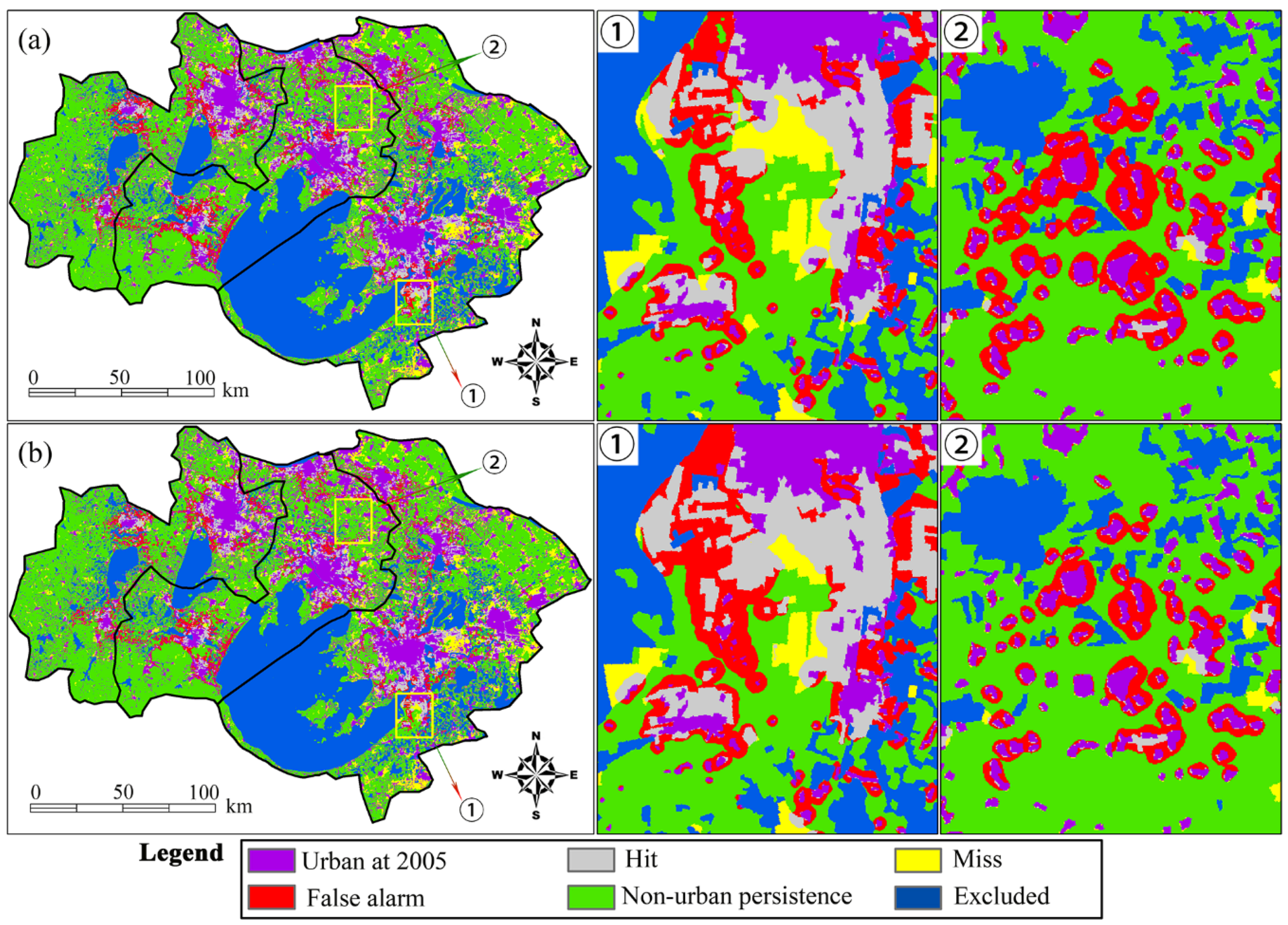
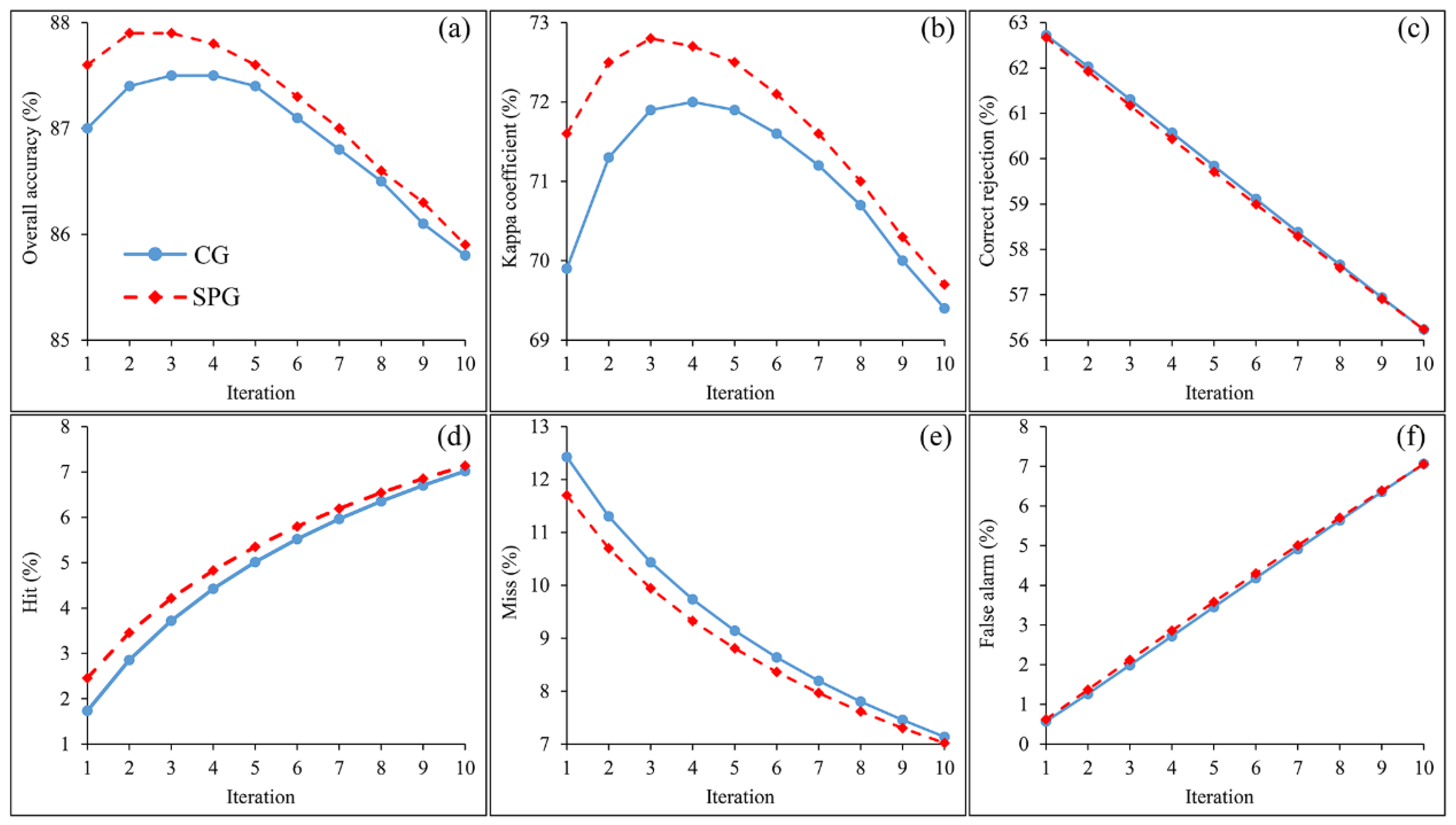
3.2.3. Accuracy and Error

Overlaying the actual and simulated urban growth maps visually demonstrates the simulation successes and errors (Figure 7), demonstrating the ability of the CA models to accurately allocate new urban cells. The overlay maps feature six categories: urban at 2005, persistent non-urban, hit, miss, false alarm and excluded. While the full maps are quite similar in simulation success and error, differences are still noticeable in the enlarged maps (the middle and right columns). In Region-1, CG-CA hit fewer cells, missed more cells and triggered fewer false alarms, while SPG-CA hit more cells, missed fewer cells and triggered more false alarms. In Region-2, no observable differences are apparent between the two models, and their simulation errors are significantly attributed to the missed new urban cells, indicating that these models hit fewer new urban cells and produced fewer false alarms in the outskirts. This suggests that both models successfully simulate the inner suburbs, but are less successful in the outer suburbs.
The six indices that represent simulation successes and errors significantly vary with the number of model iterations (Figure 8), where SPG-CA is slightly superior to CG-CA. Although the final performance of the two models is similar, there are significant differences in the simulation process. Correct rejections and false alarms are quite similar in the two models, but the other indices show distinct differences. SPG-CA yields an overall accuracy of 85.9% with a Kappa of 69.7%, while CG-CA yields an overall accuracy of 85.8% with a Kappa of 69.4%. These metrics increase, then decrease as the number of model iteration increases (Figure 8a,b). Overall accuracy peaks at the 2nd iteration for SPG-CA and at the 3rd iteration for CG-CA, while Kappa peaks at the 3rd iteration for SPG-CA and at the 4th iteration for CG-CA. With the model running, correct rejection (i.e., simulated non-urban persistence) declines while correctly simulated urban growth (hit) increases (Figure 8c,d). Figure 8d clearly shows that the hit differences between SPG-CA and CG-CA are larger when the model starts, but become smaller as the simulation progresses. Misses decrease, while false alarms increase with the model running, where the differences in misses are larger at the start than at the end.

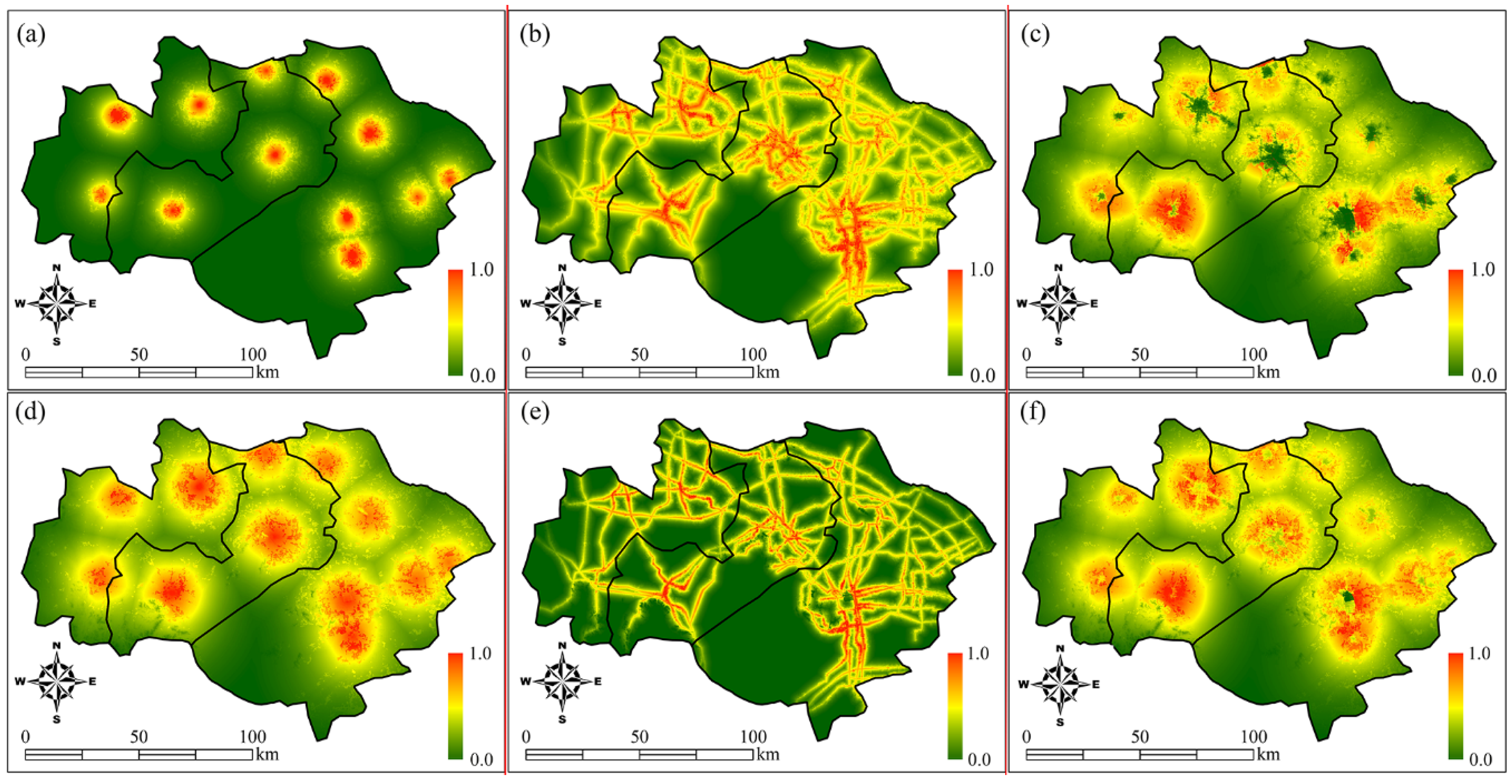
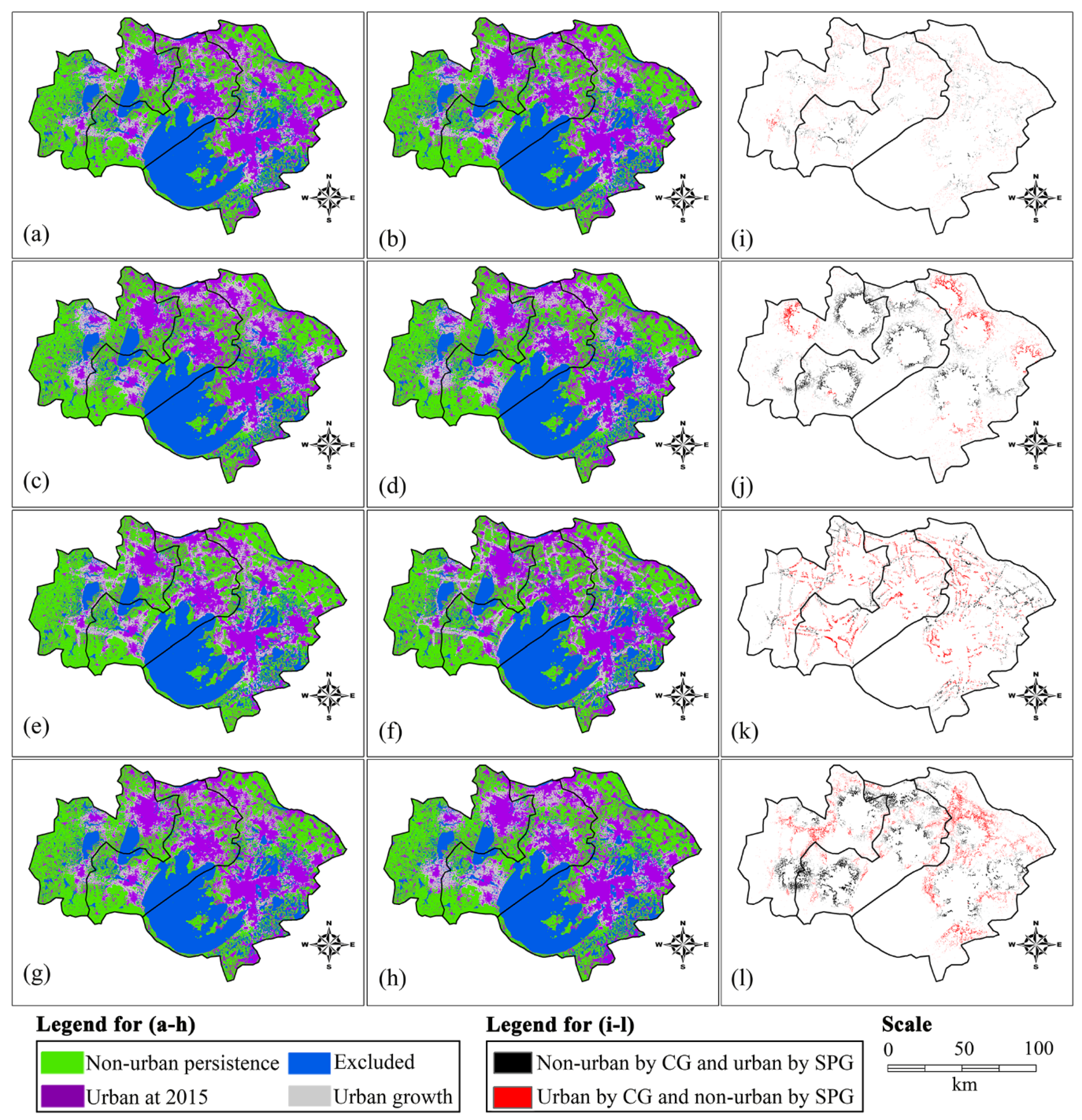
3.2.4. Future Scenario Projection

To examine the predictive power of our CA models and to explore the possibility of the urban development in Su-Xi-Chang Agglomeration, we ran four alternative 2035 simulation scenarios including BAU-scenario, COUNTY-scenario, ROAD-scenario and POP-scenario (Figure 9a–h). Our results show that there are more differences among the scenarios based on different factors than from different models. As the BAU-scenario considers all the candidate factors, the agglomeration will expand its urban extent based on the development inertia observed during 2005–2015 (Figure 9a,b). The overlay map of the two BAU-scenarios shows noticeable differences between CG-CA and SPG-CA (Figure 9i). Compared to the BAU-scenario, the COUNTY-scenario attracts more urban growth in the urban fringe of the satellite cities, but fewer in the urban fringe of Suzhou, Wuxi and Changzhou as well as along the roads that connect the central cities and satellite cities (Figure 9c,d). By comparison, CG-CA predicts more urban growth in the peri-urban areas of Zhangjiagang, Changshu and Taicang of Suzhou, and Jintan of Changzhou, whereas SPG-CA predicts more growth in the peri-urban areas of Suzhou, Wuxi, Changzhou, and Yixing of Wuxi (Figure 9j).
In the ROAD-scenario, most of the newly built-up areas occur along present road networks (Figure 9e,f), showing the incomparable effects of these networks on future urban development. By comparison, CG-CA predicts more urban growth along the arterial roads, while SPG-CA predicts more along secondary roads (Figure 9k).
The POP-scenario shows that, in the next 20 years, increased population density will lead to drastic land-use change and substantial urban growth in Liyang of Changzhou and Yixing of Wuxi, southwest of the study area (Figure 9g,h). By comparison, CG-CA predicts more urban growth in the outskirts while SPG-CA predicts more in the peri-urban areas (Figure 9l). The similarity of the COUNTY and POP factors is expected, because most residents live in the cities.
Landscape metrics should show more specific differences in area, edge, shape and aggregation spatial patterns. We used Fragstats 4.2 [56] to compute fifteen landscape metrics to describe the spatial patterns of the predicted urban patches (Table 3), where the differences between the BAU-scenario and other three scenarios are larger than those among the latter three scenarios.
The PLAND metric shows that only minor (<1%) differences exist among the scenarios, showing the ability of the CA models to control the total urban cells. The two ROAD-scenarios yield the largest urban patches, implying that the ROAD-scenarios have smaller NP and PD values (Table 3). LSI shows that, among the scenarios projected by CG-CA, the POP-scenario yields the most irregular urban shapes. Among those projected by SPG-CA, the ROAD-scenario has the most irregular urban shapes. All scenarios have the same level of patch complexity as inferred by PAFRAC. Among all scenarios, the ROAD-scenario from CG-CA has the shortest edge (18.62) while that from the SPG-CA model has the longest edge (22.03). This may be attributable to the isolated urban cells from the SPG-CA model.
The aggregation metrics indicate the tendency of urban patches to be contiguous and spatially aggregated, a general property of contagion-like phenomena. This was caused by the infilling urban development that was determined by the relatively high transition probability of a non-urban cell surrounded by other urban cells. Metrics CLUMPY, PLADJ, COHESION, DIVISION and AI show that all scenarios have uniform values across different influencing factors and CA models, and that the predicted urban patches are spatially connected and aggregated. Compared to the above five metrics, IJI shows greater difference among scenarios where the BAU-scenarios have smaller values (~69%) while the other scenarios have larger values, specially the ROAD-scenario from CG-CA. This suggests that urban land use in the BAU-scenarios is less interspersed and juxtaposed to non-urban and water while the ROAD-scenario from CG-CA is most interspersed and juxtaposed to the other land-use types. MESH is negatively related to SPLIT and thus they imply the same results. For both CA models, the ROAD-scenarios produce the largest MESH and smallest SPLIT, suggesting that these scenarios yield the largest urban patches when compared to other scenarios. This may be related to the prediction that, in the ROAD-scenarios, new urban areas along the arterial roads more completely connect the three central cities with the satellite cities.

4. Discussion

We applied five metaheuristics (Nelder-Mead, BFGS, NLMINB, CG and SPG) from the optimx package to retrieve land transition rules for the Su-Xi-Chang Agglomeration. We selected CG and SPG from these to build CA models for simulation and prediction of urban growth. We ignored Nelder-Mead, BFGS, NLMINB because they produced only minor differences as compared with CG. Both the selected metaheuristics applied box constraints in calculating the CA parameters. The 2015 simulated results yielded high overall accuracy (~86%) and Kappa exceeding 69%, suggesting that the two CA models perform well. Accuracy of the models peaked at the 3rd or 4th iterations, where they did not complete the allocation of all cells available for development. The decrease in accuracy with iteration number may be attributed to the false alarms induced during modeling. We simulated four alternative 2035 urban scenarios: business as usual and magnified effects of county centers, road networks and population density, respectively. The magnified effects adequately reflect the CA parameters from the selected metaheuristics under different box constraints.
The optimization ability of metaheuristics GA and DE may be substantially affected by the initial solution, box constraints, and controlling parameters [19,34]. All five metaheuristics might generate the same CA parameters if they employed infinite box constraints. Here, an initial solution and box constraints were based on parameters derived from LR. A recent publication [20] shows that box constraints can also be defined using extensive tests that produce similar results. Compared to metaheuristics that do not employ box constraints, box-constrained metaheuristics are more efficient in optimization [66], and they produce repeatable CA parameters. Our pre-examination also shows that CG and SPG are less sensitive to the change in their controlling parameters, suggesting robustness in establishing urban CA models.
Similarity in land transition probability maps suggests similarity in spatial patterns of the simulations. Our CG-CA and SPG-CA models successfully capture urban growth in three major cities (the Suzhou, Wuxi and Changzhou city centers), whereas they are less able to model small patches of urban growth in the outskirts and satellite cities. Moreover, the simulated urban patches lost some spatial details and are smoother than the actual patches, an inherent issue in CA modeling [67]. CA is essentially a moving-window method of spatial analysis. As such, the state of each cell is affected by its surrounding cells; effectively this is a smoothing filter. We therefore suggest that adding landscape heterogeneity into CA modeling could eliminate this smoothing effect.
In addition to minimizing the residuals and automatically searching for CA parameters, another advantage of metaheuristics is that complex conditions (i.e., equality and inequality constraints for the fitness function and box-constraints for the CA parameters) can be taken into account during optimization [68]. As such, metaheuristics generate different CA parameters that express the physical constraints required to predict urban future scenarios. This means it is possible to quickly solve minimization problems with complex constraints using metaheuristics such as PSO, SA, DE, CG, SPG and Nelder-Mead. Metaheuristics feature objective parameterization of transition rules for scenario prediction [19], as compared with the LR method. These scenarios should inform modelers and policy-makers about how the Su-Xi-Chang Agglomeration might evolve over the next 20 years when considering only one factor at a time. Our CA-based scenario prediction is of practical significance for assessing the consequences of macroeconomic policy and urban planning regulations as well as tuning their future directions. For example, planners can use our models to identify possible future illegal (unplanned) development and estimate urban-encroachment on agricultural and ecologically valuable land, hence evaluating the negative effect of urban growth on ecosystems, environments, and regional climate.
Overall, our major contribution is the development of a set of comparable urban CA models using the R package optimx. These models are featured by the prediction ability in modeling urban future scenarios in response to different development strategies and policies. This model feature is based on objective parameterization that has not been adequately addressed in previous studies. Our models can also be used to simulate multiple land-use change. The use of R package optimx facilitates other model developers to easily follow our methods for their specific applications elsewhere. Limitations exist in our models because they can be affected by their own controlling parameters, in which appropriate parameterization needs experience of mastering intelligent algorithms or extensive tests. In addition, the principal limitation of these models is that they generate urban patches that are smoother than the actual urban patterns.

5. Conclusions

The R package optimx provides a unified framework (with many alternatives) that is suitable for solving optimization problems. We developed five CA models for simulating urban growth using the metaheuristics included in optimx, which automatically search for the near-optimal parameters in defining land transition rules. We selected CG and SPG to simulate 2005–2015 urban growth and projected 2035 scenarios for the Su-Xi-Chang Agglomeration of Jiangsu Province. The CG-CA and SPG-CA models we constructed yielded high overall accuracies of about 86% and Kappa coefficients exceeding 69%, indicating their strong ability of urban growth simulation. Compared to other methods based on statistical techniques and fuzzy sets, the competitive advantage of metaheuristics is its strong ability to solve complex constrained problems, resulting in objective parameterization with strong predictive power. We simulated four alternative 2035 urban scenarios by considering the effects of all land use change drivers as well as the magnified effects of county centers, road networks and population density. These scenarios provide insights into future urban patterns resulting from current urban planning and infrastructure, and can inform advisable development strategies for sustainable cities.
Our metaheuristic CA models are readily applicable to modeling land use and urban growth in rapidly developing areas. The principal limitation of these models is that they generate urban patches that are smoother than the actual urban patterns. We suggest that incorporating landscape heterogeneity into the CA models may reduce this smoothing effect. Future studies should focus on [1] spatial visualization of landscape heterogeneity, [2] a method to integrate heterogeneity into CA models, and [3] the performance of heterogeneous CA models. This could eliminate the contagion-like phenomena that are common in CA-based urban modeling. In addition, climate change and more socioeconomic factors should be considered in CA modeling to address the complex impacts of the natural and human effects on the regional and global urban growth. These should promote the progress of CA research in both modeling methods and application.

Author Contributions

Conceptualization, Y.F.; methodology, Y.F. and Z.C.; software, Y.F. and Z.C.; validation, J.W., C.G., S.C. and Z.L.; formal analysis, Y.F. and Z.C.; investigation, Z.C.; resources, J.W., C.G., S.C. and Z.L.; data curation, Y.F. and Z.C.; writing—original draft preparation, Z.C.; writing—review and editing, Y.F. and X.T.; visualization, J.W., C.G., S.C. and Z.L.; supervision, Y.F. and X.T.; project administration, Y.F.; funding acquisition, Y.F. and X.T.

Funding

This study was supported by the National Natural Science Foundation of China (No. 41631178 and No. 41771414) and the National Key R&D Program of China (No. 2018YFB0505400 and No. 2018YFB0505402).

Acknowledgments

We would like to thank three anonymous reviewers for their constructive comments and efforts to improve the manuscript.

Conflicts of Interest

The authors declare no conflict of interest.

References

  1. Herold, M.; Goldstein, N.C.; Clarke, K.C. The spatiotemporal form of urban growth: Measurement, analysis and modeling. Remote Sens. Environ. 2003, 86, 286–302. [Google Scholar] [CrossRef]
  2. Rimal, B.; Zhang, L.; Keshtkar, H.; Haack, B.N.; Rijal, S.; Zhang, P. Land use/land cover dynamics and modeling of urban land expansion by the integration of cellular automata and markov chain. ISPRS Int. J. Geo-Inf. 2018, 7, 154. [Google Scholar] [CrossRef]
  3. Arsanjani, J.J.; Helbich, M.; Kainz, W.; Boloorani, A.D. Integration of logistic regression, markov chain and cellular automata models to simulate urban expansion. Int. J. Appl. Earth Obs. Geoinf. 2013, 21, 265–275. [Google Scholar] [CrossRef]
  4. Santé, I.; García, A.M.; Miranda, D.; Crecente, R. Cellular automata models for the simulation of real-world urban processes: A review and analysis. Landsc. Urban Plan. 2010, 96, 108–122. [Google Scholar] [CrossRef]
  5. Liu, Y.; Feng, Y. Simulating the impact of economic and environmental strategies on future urban growth scenarios in Ningbo, China. Sustainability 2016, 8, 1045. [Google Scholar] [CrossRef]
  6. Feng, Y.; Li, H.; Tong, X.; Chen, L.; Liu, Y. Projection of land surface temperature considering the effects of future land change in the Taihu Lake Basin of China. Glob. Planet. Chang. 2018, 167, 24–34. [Google Scholar] [CrossRef]
  7. Li, X.; Yeh, A.G.-O. Modelling sustainable urban development by the integration of constrained cellular automata and GIS. Int. J. Geogr. Inf. Sci. 2000, 14, 131–152. [Google Scholar] [CrossRef] [Green Version]
  8. Toffoli, T.; Margolus, N. Cellular Automata Machines: A New Environment for Modeling; MIT Press: Cambridge, MA, USA, 1987. [Google Scholar]
  9. Wu, F. Simland: A prototype to simulate land conversion through the integrated GIS and CA with AHP-derived transition rules. Int. J. Geogr. Inf. Sci. 1998, 12, 63–82. [Google Scholar] [CrossRef]
  10. Feng, Y.; Liu, M.; Chen, L.; Liu, Y. Simulation of dynamic urban growth with partial least squares regression-based cellular automata in a GIS environment. ISPRS Int. J. Geo-Inf. 2016, 5, 243. [Google Scholar] [CrossRef]
  11. Yu, Y.; He, J.; Tang, W.; Li, C. Modeling urban collaborative growth dynamics using a multiscale simulation model for the Wuhan urban agglomeration area, China. ISPRS Int. J. Geo-Inf. 2018, 7, 176. [Google Scholar] [CrossRef]
  12. Liu, X.; Li, X.; Shi, X.; Huang, K.; Liu, Y. A multi-type ant colony optimization (MACO) method for optimal land use allocation in large areas. Int. J. Geogr. Inf. Sci. 2012, 26, 1325–1343. [Google Scholar] [CrossRef]
  13. Torrens, P.M.; O’Sullivan, D. Cellular automata and urban simulation: Where do we go from here? Environ. Plan. B 2001, 28, 163–168. [Google Scholar] [CrossRef]
  14. Feng, Y.; Tong, X. Dynamic land use change simulation using cellular automata with spatially nonstationary transition rules. GISci. Remote Sens. 2018, 55, 678–698. [Google Scholar] [CrossRef]
  15. Maria de Almeida, C.; Batty, M.; Vieira Monteiro, A.M.; Câmara, G.; Soares-Filho, B.S.; Cerqueira, G.C.; Pennachin, C.L. Stochastic cellular automata modeling of urban land use dynamics: Empirical development and estimation. Comput. Environ. Urban Syst. 2003, 27, 481–509. [Google Scholar] [CrossRef]
  16. Laumanns, M.; Thiele, L.; Zitzler, E. An efficient, adaptive parameter variation scheme for metaheuristics based on the epsilon-constraint method. Eur. J. Oper. Res. 2006, 169, 932–942. [Google Scholar] [CrossRef] [Green Version]
  17. Feng, Y.; Tong, X. Calibration of cellular automata models using differential evolution to simulate present and future land use. Trans. GIS 2018, 22, 582–601. [Google Scholar] [CrossRef]
  18. Kamusoko, C.; Gamba, J. Simulating urban growth using a random forest-cellular automata (RF-CA) model. ISPRS Int. J. Geo-Inf. 2015, 4, 447–470. [Google Scholar] [CrossRef]
  19. Jafarnezhad, J.; Salmanmahiny, A.; Sakieh, Y. Subjectivity versus objectivity: Comparative study between brute force method and genetic algorithm for calibrating the SLEUTH urban growth model. J. Urban Plan. Dev. 2015, 142, 05015015. [Google Scholar] [CrossRef]
  20. Feng, Y.; Liu, Y.; Tong, X. Comparison of metaheuristic cellular automata models: A case study of dynamic land use simulation in the Yangtze River Delta. Comput. Environ. Urban Syst. 2018, 70, 138–150. [Google Scholar] [CrossRef]
  21. Yang, J.; Tang, G.A.; Cao, M.; Zhu, R. An intelligent method to discover transition rules for cellular automata using bee colony optimisation. Int. J. Geogr. Inf. Sci. 2013, 27, 1849–1864. [Google Scholar] [CrossRef]
  22. Yang, X.; Zheng, X.-Q.; Lv, L.-N. A spatiotemporal model of land use change based on ant colony optimization, markov chain and cellular automata. Ecol. Model. 2012, 233, 11–19. [Google Scholar] [CrossRef]
  23. Cao, M.; Bennett, S.J.; Shen, Q.; Xu, R. A bat-inspired approach to define transition rules for a cellular automaton model used to simulate urban expansion. Int. J. Geogr. Inf. Sci. 2016, 30, 1961–1979. [Google Scholar] [CrossRef]
  24. Almeida, C.d.; Gleriani, J.; Castejon, E.F.; Soares-Filho, B. Using neural networks and cellular automata for modelling intra-urban land-use dynamics. Int. J. Geogr. Inf. Sci. 2008, 22, 943–963. [Google Scholar] [CrossRef]
  25. Rienow, A.; Goetzke, R. Supporting sleuth–enhancing a cellular automaton with support vector machines for urban growth modeling. Comput. Environ. Urban Syst. 2015, 49, 66–81. [Google Scholar] [CrossRef]
  26. Nesmachnow, S. An overview of metaheuristics: Accurate and efficient methods for optimisation. Int. J. Metaheuristics 2014, 3, 320–347. [Google Scholar] [CrossRef]
  27. Barredo, J.I.; Kasanko, M.; McCormick, N.; Lavalle, C. Modelling dynamic spatial processes: Simulation of urban future scenarios through cellular automata. Landsc. Urban Plan. 2003, 64, 145–160. [Google Scholar] [CrossRef]
  28. Liu, X.; Li, X.; Shi, X.; Zhang, X.; Chen, Y. Simulating land-use dynamics under planning policies by integrating artificial immune systems with cellular automata. Int. J. Geogr. Inf. Sci. 2010, 24, 783–802. [Google Scholar] [CrossRef]
  29. Basse, R.M.; Omrani, H.; Charif, O.; Gerber, P.; Bódis, K. Land use changes modelling using advanced methods: Cellular automata and artificial neural networks. The spatial and explicit representation of land cover dynamics at the cross-border region scale. Appl. Geogr. 2014, 53, 160–171. [Google Scholar] [CrossRef]
  30. Newland, C.P.; Maier, H.R.; Zecchin, A.C.; Newman, J.P.; van Delden, H. Multi-objective optimisation framework for calibration of cellular automata land-use models. Environ. Model. Softw. 2018, 100, 175–200. [Google Scholar] [CrossRef]
  31. Nash, J.C.; Varadhan, R. Unifying optimization algorithms to aid software system users: Optimx for R. J. Stat. Softw. 2011, 43, 1–14. [Google Scholar] [CrossRef]
  32. Nash, J.C. On best practice optimization methods in R. J. Stat. Softw. 2014, 60, 1–14. [Google Scholar] [CrossRef]
  33. Wu, F. Calibration of stochastic cellular automata: The application to rural-urban land conversions. Int. J. Geogr. Inf. Sci. 2002, 16, 795–818. [Google Scholar] [CrossRef]
  34. Li, X.; Yang, Q.; Liu, X. Genetic algorithms for determining the parameters of cellular automata in urban simulation. Sci. China Ser. D Earth Sci. 2007, 50, 1857–1866. [Google Scholar] [CrossRef]
  35. Duthie, J.; Kockelman, K.; Valsaraj, V.; Zhou, B. Applications of integrated models of land use and transport: A comparison of itlup and urbansim land use models. In Proceedings of the 54th Annual North American Meetings of the Regional Science Association International, Savannah, GA, USA, 7–11 November 2007. [Google Scholar]
  36. Nagy, J.; Bardsley, J.; Plemmons, R.; Jefferies, S. A computational method for the restoration of images with an unknown, spatially-varying blur. Opt. Express 2006, 14, 1767–1782. [Google Scholar]
  37. Brooks, C.P.; Holmes, C.; Kramer, K.; Barnett, B.; Keitt, T.H. The role of demography and markets in determining deforestation rates near Ranomafana national park, Madagascar. PLoS ONE 2009, 4, e5783. [Google Scholar] [CrossRef] [PubMed] [Green Version]
  38. Guan, Q.; Wang, L.; Clarke, K.C. An artificial-neural-network-based, constrained CA model for simulating urban growth. Am. Cartogr. 2005, 32, 369–380. [Google Scholar] [CrossRef]
  39. Shen, D.; Blasch, E.; Pham, K.; Chen, G.; Ling, H. Spatial Context for Moving Vehicle Detection in Wide Area Motion Imagery with Multiple Kernel Learning. Proc. SPIE 2013, 8751, doi. [Google Scholar]
  40. Price, K.; Storn, R.M.; Lampinen, J.A. Differential Evolution: A Practical Approach to Global Optimization; Springer Science & Business Media: Berlin, Germany, 2006. [Google Scholar]
  41. Li, D.; Fukushima, M. On the global convergence of the BFGS method for nonconvex unconstrained optimization problems. SIAM J. Optimiz. 2001, 11, 1054–1064. [Google Scholar] [CrossRef]
  42. Liao, A. Modifying the BFGS method. Oper. Res. Lett. 1997, 20, 171–177. [Google Scholar] [CrossRef]
  43. Lewis, A.S.; Overton, M.L. Nonsmooth Optimization via Bfgs. Available online: https://www.semanticscholar.org/paper/Nonsmooth-Optimization-via-Bfgs-Overton/9e9db481d16bc409abc95853687f3fd7e1784641 (accessed on 28 April 2018).
  44. Gay, D.M. Usage Summary for Selected Optimization Routines; Computing Science Technical Report No. 153; AT&T Bell Laboratories: Murray Hill, NJ, USA, 1990. [Google Scholar]
  45. Ardia, D.; David, J.; Arango, O.; Gómez, N.D.G. Jump-diffusion calibration using differential evolution. Wilmott 2011, 2011, 76–79. [Google Scholar] [CrossRef] [Green Version]
  46. Thmasebinejad, Z.; Tabrizi, E. Sensitivity analysis in correlated bivariate continuous and binary responses. Appl. Appl. Math. Int. J. 2015, 10, 609–619. [Google Scholar]
  47. Nikishin, A.A.; Yeremin, A.Y. Variable block cg algorithms for solving large sparse symmetric positive definite linear systems on parallel computers, i: General iterative scheme. SIAM J. Matrix Anal. Appl. 1995, 16, 1135–1153. [Google Scholar] [CrossRef]
  48. Gergelits, T.; Strakoš, Z. Composite convergence bounds based on chebyshev polynomials and finite precision conjugate gradient computations. Numer. Algorithms 2014, 65, 759–782. [Google Scholar] [CrossRef]
  49. Birgin, E.G.; Martínez, J.M.; Raydan, M. Spectral projected gradient methods: Review and perspectives. J. Stat. Softw. 2014, 60, 1–21. [Google Scholar] [CrossRef]
  50. Pontius, R.G.; Parmentier, B. Recommendations for using the relative operating characteristic (ROC). Landsc. Ecol. 2014, 29, 367–382. [Google Scholar] [CrossRef]
  51. Pontius, R.G.; Si, K. The total operating characteristic to measure diagnostic ability for multiple thresholds. Int. J. Geogr. Inf. Sci. 2014, 28, 570–583. [Google Scholar] [CrossRef]
  52. Pontius, R.G.; Shusas, E.; McEachern, M. Detecting important categorical land changes while accounting for persistence. Agric. Ecosyst. Environ. 2004, 101, 251–268. [Google Scholar] [CrossRef]
  53. Pontius, R.G.; Boersma, W.; Castella, J.-C.; Clarke, K.; de Nijs, T.; Dietzel, C.; Duan, Z.; Fotsing, E.; Goldstein, N.; Kok, K. Comparing the input, output, and validation maps for several models of land change. Ann. Reg. Sci. 2008, 42, 11–37. [Google Scholar] [CrossRef]
  54. Congalton, R.G. A review of assessing the accuracy of classifications of remotely sensed data. Remote Sens. Environ. 1991, 37, 35–46. [Google Scholar] [CrossRef]
  55. Vanbelle, S.; Albert, A. A note on the linearly weighted kappa coefficient for ordinal scales. Stat. Methodol. 2009, 6, 157–163. [Google Scholar] [CrossRef] [Green Version]
  56. McGarigal, K. Fragstats v4: Spatial Pattern Analysis Program for Categorical and Continuous Maps-Help Manual; University of Massachusetts: Amherst, MA, USA, 2014. [Google Scholar]
  57. Dunn, J.C. Spatial metrics of integral and separable dimensions. J. Exp. Psychol. Hum. Percept. Perform. 1983, 9, 242. [Google Scholar] [CrossRef] [PubMed]
  58. Lu, S.; Guan, X.; Zhou, M.; Wang, Y. Land resources allocation strategies in an urban area involving uncertainty: A case study of suzhou, in the Yangtze River Delta of China. Environ. Manag. 2014, 53, 894–912. [Google Scholar] [CrossRef] [PubMed]
  59. Zhang, N.; Gao, Z.; Wang, X.; Chen, Y. Modeling the impact of urbanization on the local and regional climate in Yangtze River Delta, China. Theor. Appl. Climatol. 2010, 102, 331–342. [Google Scholar] [CrossRef]
  60. Feng, Y.; Tong, X. Using exploratory regression to identify optimal driving factors for cellular automaton modeling of land use change. Environ. Monit. Assess. 2017, 189, 515. [Google Scholar] [CrossRef] [PubMed]
  61. National Earth System Science Data Sharing Infrastructure. Available online: www.geodata.cn (accessed on 28 April 2018).
  62. Geospatial Data Cloud. Available online: www.gscloud.cn (accessed on 28 April 2018).
  63. WorldPop. Available online: worldpop.org.uk (accessed on 28 April 2018).
  64. Liu, X.; Liang, X.; Xu, X.; Ou, J.; Li, X.; Chen, Y.; Li, S.; Wang, S.; Pei, F. A future land use simulation model (FLUS) for simulating multiple land use scenarios by coupling human and natural effects. Landsc. Urban Plan. 2017, 168, 94–116. [Google Scholar] [CrossRef]
  65. Gounaridis, D.; Chorianopoulos, I.; Koukoulas, S. Exploring prospective urban growth trends under different economic outlooks and land-use planning scenarios: The case of Athens. Appl. Geogr. 2018, 90, 134–144. [Google Scholar] [CrossRef]
  66. Liberti, L.; Drazic, M. Variable Neighbourhood Search for the Global Optimization of Constrained NLPs; Proceedings of the GO Workshop: Almeria, Spain, 2005. [Google Scholar]
  67. Wolfram, S. Cellular automata as models of complexity. Nature 1984, 311, 419. [Google Scholar] [CrossRef]
  68. Chowdhury, S.; Zhang, J.; Messac, A.; Castillo, L. Characterizing the influence of land configuration on the optimal wind farm performance. In Proceedings of the ASME 2011 International Design Engineering Technical Conferences and Computers and Information in Engineering Conference, Washington, DC, USA, 28–31 August 2011; American Society of Mechanical Engineers: New York, NY, USA, 2011; pp. 367–378. [Google Scholar]
Figure 1. Study areas: (a) China, (b) Jiangsu Province, and (c) Administrative boundary of the Su-Xi-Chang Agglomeration.
Ijgi 07 00387 g001
Figure 2. The urban patterns in 2005 and 2015 classified using Landsat images. (a) Urban pattern in 2005, and (b) Urban pattern in 2015.
Ijgi 07 00387 g002
Figure 3. Driving factors for metaheuristic CA models. (a) Distance to city centers (CITY), (b) Distance to county centers (COUNTY), (c) Distances to arterial roads (ROAD), (d) Distances to railway (RAIL), (e) Digital elevation model (DEM) data, and (f) Population density (POP).
Ijgi 07 00387 g003
Figure 4. Land transition probability maps and their differences. (a) Land transition probability from Nelder-Mead, BFGS and CG, (b) Land transition probability from NLMINB, (c) Land transition probability from SPG, (d) Probability differences (a minus b), (e) Probability differences (a minus c), and (f) Probability differences (b minus c).
Ijgi 07 00387 g004
Figure 5. Land transition probability maps for scenario prediction based on CG and SPG. (a) Land transition probability by CG for COUNTY-scenario, (b) Land transition probability by CG for ROAD-scenario, (c) Land transition probability by CG for POP-scenario, (d) Land transition probability by SPG for COUNTY-scenario, (e) Land transition probability by SPG for ROAD-scenario, and (f) Land transition probability by SPG for POP-scenario.
Ijgi 07 00387 g005
Figure 6. The simulated 2015 urban patterns with two enlarged regions showing local differences. (a) 2015 simulated result by CG, and (b) 2015 simulated result by SPG.
Ijgi 07 00387 g006
Figure 7. Maps of simulation successes and errors for conjugate gradient-based CA (CG-CA) and spectral projected gradient-based CA (SPG-CA) models. (a) Simulation successes and errors of CG, and (b) Simulation successes and errors of SPG.
Ijgi 07 00387 g007
Figure 8. Changes in simulation success and error during the simulation. (a) Overall accuracy, (b) kappa coefficient, (c) correct rejection, (d) hit, (e) miss, and (f) false alarm.
Ijgi 07 00387 g008
Figure 9. Urban scenarios for 2035 predicted using both the CG-CA and SPG-CA models. (a) BUA-scenario by CG-CA, (b) BUA-scenario by SPG-CA, (c) COUNTY-scenario by CG-CA, (d) COUNTY-scenario by SPG-CA, (e) ROAD-scenario by CG-CA, (f) ROAD-scenario by SPG-CA, (g) POP-scenario by CG-CA, (h) POP-scenario by SPG-CA, (i) comparison of BAU-scenarios between CG and SPG, (j) comparison of COUNTY-scenarios between CG and SPG, (k) comparison of ROAD-scenarios between CG and SPG, and (l) comparison of POP-scenarios between CG and SPG.
Ijgi 07 00387 g009
Table 1. Upper and lower box constraints and CA parameters for each metaheuristic. Abbreviations: Nonlinear Minimization in Box Constraints (NLMINB); Broyden-Fletcher-Goldfarb-Shanno (BFGS); conjugate gradients (CG); spectral projected gradient (SPG).
VariableBoundParameter
LowerUpperNelder-MeadBFGSNLMINBCGSPG
Constant (a0)0.02.52.35012.35012.35712.35011.2259
CITY (a1)−1.50.0−1.2328−1.2328−1.235−1.2328−1.1847
COUNTY (a2)−2.50.0−2.3400−2.3400−2.3378−2.3400−2.3602
ROAD (a6)−5.50.0−5.0887−5.0887−5.1342−5.0887−5.2511
RAIL (a5)0.01.00.49870.49870.50050.49870.4815
DEM (a3)−25.00.0−24.4068−24.4068−24.4449−24.4068−14.9771
POP (a4)−2.50.0−2.0799−2.0799−2.0898−2.0799−2.1664
Table 2. Upper and lower box constraints and CA parameters for each metaheuristic.
VariableCGSPG
COUNTY-ScenarioROAD-ScenarioPOP-ScenarioCOUNTY-ScenarioROAD-ScenarioPOP-Scenario
Constant (a0)−0.1281−0.64510.1698−0.63840.6875−0.2087
CITY (a1)−0.4885−1.1616−0.9569−0.4898−1.4611−0.9365
COUNTY (a2) 11.3422 −1.9124−4.6545 3.8768 −2.3049−3.8563
ROAD (a6)−0.1621 8.6481 −0.6391−0.5234 20.1010 −0.5387
RAIL (a5)1.21140.6510−1.17290.01750.7939−0.4839
DEM (a3)−0.44860.1688−1.0863−1.2922−6.7003−1.6566
POP (a4)0.57010.9831 18.5703 −0.1517−3.0661 4.9698
Table 3. Landscape metrics of the urban class of the four alternative urban scenarios. Abbreviations: percentage of landscape (PLAND); largest patch index (LPI); total edge (TE); perimeter-area fractal dimension (PAFRAC); number of patches (NP); patch density (PD); landscape shape index (LSI); clumpiness index (CLUMPY); percentage of like adjacencies (PLADJ); patch cohesion index (COHESION); landscape division index (DIVISION); aggregation index (AI); interspersion and juxtaposition index (IJI); effective mesh size (MESH); and splitting index (SPLIT).
CategoryMetricCGSPG
BAU-ScenarioCOUNTY-ScenarioROAD-ScenarioPOP-ScenarioBAU-ScenarioCOUNTY-ScenarioROAD-ScenarioPOP-Scenario
Area and EdgePLAND (%)38.3537.9738.6638.6238.2538.7938.4238.65
LPI (%)7.688.4913.688.597.728.8916.118.80
TE (1000 km)20.8721.0018.6221.5421.3021.1122.0321.15
ShapePAFRAC1.251.241.241.251.261.261.281.25
AggregationNP (num)54935821535755285588555555985540
PD (num/km2)0.320.340.310.320.320.320.320.32
LSI (%)64.6365.4257.3866.4666.0365.0168.1565.22
CLUMPY (%)0.960.960.970.960.960.960.960.96
PLADJ (%)97.6297.5897.8997.5697.5697.6297.4997.61
COHESION (%)99.7299.6899.8399.7599.7299.7299.8699.76
DIVISION (%)0.990.990.970.980.990.990.960.98
AI (%)97.6697.6197.9397.6097.6097.6597.5397.64
IJI (%)69.2572.0977.0471.3269.7873.3469.7471.86
MESH (ha)2.532.185.423.202.562.516.843.39
SPLIT68.2579.2931.9254.1067.5568.8525.2950.95

