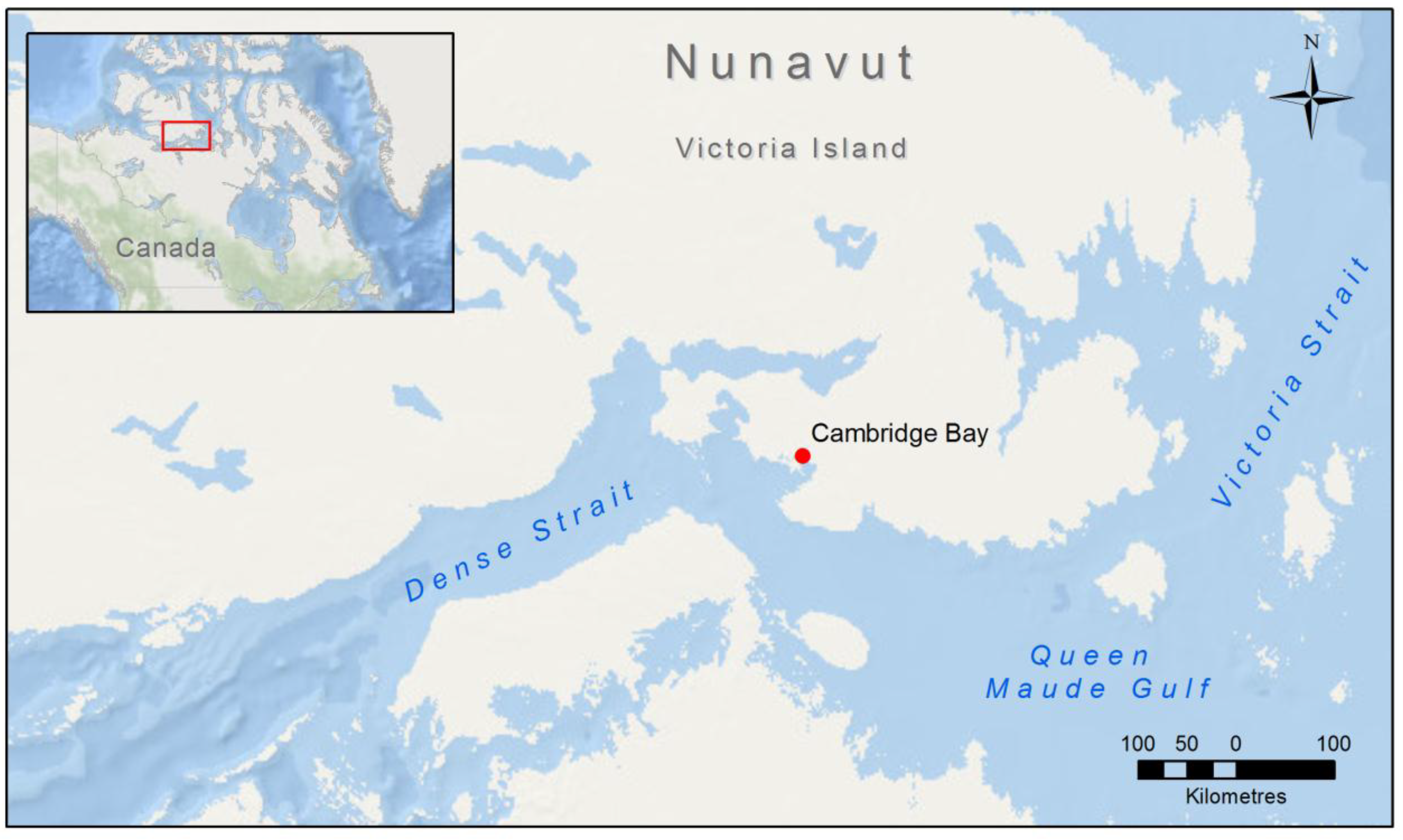
Article

Bathymetric Photogrammetry to Update CHS Charts: Comparing Conventional 3D Manual and Automatic Approaches

Canadian Hydrographic Service, 200 Kent Street, Ottawa, ON K1A 0E6, Canada
*
Author to whom correspondence should be addressed.
ISPRS Int. J. Geo-Inf. 2018, 7(10), 395; https://0-doi-org.brum.beds.ac.uk/10.3390/ijgi7100395
Submission received: 22 June 2018 / Revised: 8 September 2018 / Accepted: 23 September 2018 / Published: 2 October 2018

Abstract

:
The Canadian Hydrographic Service (CHS) supports safe navigation within Canadian waters through approximately 1000 navigational charts as well as hundreds of publications. One of the greatest challenges faced by the CHS is removing gaps in bathymetric survey data, particularly in the Canadian Arctic where only 6% of navigational water is surveyed to modern standards. Therefore, the CHS has initiated a research project to explore remote sensing methods to improve Canadian navigational charts. The major components of this project explore satellite derived bathymetry (SDB), coastline change detection and coastline extraction. This paper focuses on the potential of two stereo satellite techniques for deriving SDB: (i) automatic digital elevation model (DEM) extraction using a semi-global matching method, and (ii) 3D manual delineation of depth contours using visual stereoscopic interpretation. Analysis focused on quantitative assessment which compared estimated depths from both automatic and 3D manual photogrammetric approaches against available in situ survey depths. The results indicate that the 3D manual approach provides an accuracy of <2 m up to a depth of 15 m. Comparable results were obtained from the automatic approach to a depth of 12 m. For almost all investigated depth ranges for both techniques, uncertainties were found to be within the required vertical accuracies for the International Hydrographic Organization category zone of confidence (CATZOC) level C classification for hydrographic surveys. This indicates that both techniques can be used to derive navigational quality bathymetric information within the investigated study site. While encouraging, neither technique was found to offer a single solution for the complete estimation of depth within the study area. As a result of these findings, the CHS envisions a hybrid approach where stereo- and reflectance-based bathymetry estimation techniques are implemented to provide the greatest understanding of depth possible from satellite imagery. Overall, stereo photogrammetry techniques will likely allow for new potential for supporting the improvement of CHS charts in areas where modern surveys have not yet been obtained.

1. Introduction

Under the authority delegated to Fisheries and Oceans Canada under the Oceans Act, the Canadian Hydrographic Service (CHS) is responsible for providing hydrographic products and services to ensure the safe, sustainable and navigable use of Canada’s waterways. The CHS is responsible for the production and maintenance of approximately 1000 nautical charts and other hydrographic publications. With a length of over 243,700 km, Canada has the longest coastline of any country in the world [1]. Charting Canadian waters and ensuring that all nautical products are up-to-date is thus a challenging task for the CHS. The required effort is even greater in the Canadian Arctic as the remoteness, climatic conditions and short summer season reduce opportunities to collect bathymetric data. The impact of these factors directly contributes to the sparse coverage of modern hydrographic surveys in the Arctic, which account for only 6% of Arctic waters.
To enable the organization to fill data gaps both in the Arctic and across all Canadian waters, the CHS, through a Canadian Space Agency (CSA) Government Related Initiatives Program (GRIP) project, is exploring remote sensing techniques as an alternative source of accurate and reliable hydrographic data. The datasets generated from remote sensing would directly contribute to an improvement in quality of CHS navigational charts. The project is specifically leveraging a hybrid optical/synthetic aperture radar (SAR) shoreline extraction and change detection approach, as well as optical satellite derived bathymetry (SDB) methodologies. Under the GRIP project, it was proposed to evaluate SDB techniques such as photogrammetric, empirical and classification approaches [2]. It is highly beneficial to carry out research to improve SDB, since traditional depth extraction surveys are expensive, time consuming and contain inherent safety risks, particularly in shallow water.
While SDB has been around for over 40 years [3], most of the development has focused on reflectance-based approaches, e.g., [4,5,6,7,8,9,10]. These approaches leverage the simple fact that, as given by Beer’s law, light is attenuated as it travels through the water column. Therefore, as depth increases, the water leaving radiance (Lw: W m−2 μm−1 sr−1) decreases until optically deep waters (i.e., where Lw has no noticeable contribution from the seafloor) are reached. Thus, a link can be created between Lw (or reflectance from the water pixel [Rw: unitless] if Lw is scaled to the downwelling irradiance at the surface of the water [Ed(0+): W m−2 μm−1 sr−1]) and depth either empirically [4,5,6,8] or through physical modeling [7,9,10].
Generally, these reflectance-based approaches can extract bathymetry with ~1 m of accuracy to depths of up to 40 m in ideal conditions [11]. However, they often struggle to retrieve bathymetric information over heterogeneous zones [2]. This is mainly a result of areas with lower albedo being quite similar to optically deep waters. This is more problematic with approaches that seek to identify a central trend, e.g., [4,8], leading to an overestimation of depths over darker areas. Hence, these approaches are better tuned to perform well in homogeneous areas of high albedo substrate (e.g., sand).
Another approach to extract bathymetry from space-based Earth observation (EO) is through the analysis of wave propagation over near-shore areas (i.e., wave kinematics bathymetry: WKB). As waves travel from areas of deeper to shallower water, they interact with the seafloor and thus slow down, causing the wavelength to decrease [12]. This principle has led to the development of several methods to infer bathymetry based on the surface signatures of currents and waves, e.g., [13,14,15]. With sufficiently large waves, some of these approaches can work to about an 80 m depth, though there have been studies showing that deep ocean topography signatures can be identified under optimal conditions [16], enabling these approaches to capture significantly deeper depths than reflectance-based approaches. While WKB is promising, there are also several drawbacks to the methodology that limit its applicability. The requirement of ideal wave conditions limits the number of usable scenes. Another more important limitation is the relative accuracy, which thus far has been found to be less than what is expected from reflectance-based bathymetry. For instance, Danilo and Melgani [16] managed to obtain root mean square errors (RMSEs) of approximately 5 m in up to 20 m of water; Mancini et al. [17] at best achieved results within <1 m of error for depths from 4 to 8 m, but the error grew rapidly both below and beyond that range.
This work focuses on a more recent approach for SDB: stereo photogrammetry. Likely best known for its wide use in generating digital elevation models (DEM) of the Earth’s entire landmass, e.g., [18], only limited research has been completed to investigate the potential of stereo photogrammetry for deriving water depth, most recently by Hodul et al. [19]. As opposed to reflectance and WKB SDB approaches, stereo photogrammetry is not sensitive to variations in the substrate reflectance or water conditions (in so far as these variations do not obstruct visibility of the seafloor). Consequently, it is of particular interest to the CHS as a valuable tool to supplement depths obtained from traditional hydrographic surveys in areas where other traditional SDB approaches are less reliable.
The main objective of this research was to examine the potential of stereoscopic approaches for bathymetry extraction using high resolution optical datasets. This paper examines the results obtained using two photogrammetric approaches: an automatic image correlation approach, and manual visual feature extraction.

2. Study Area and Datasets

2.1. Study Area

This research focuses on an area near Cambridge Bay, Nunavut, in the Canadian Arctic (Figure 1). The water in Cambridge Bay is generally clear and the bottom is composed mostly of sand and rock. However, the sea floor environment is more heterogeneous with numerous patches of vegetation. The tidal range at Cambridge Bay is small, with high tides rarely reaching more than 0.4 m above chart datum.
For northern countries such as Canada, one of the major limiting factors in SDB generation is the sun angle. For Cambridge Bay (69° N), the optimum sun elevation angle is approximately 43°, which occurs during the summer solstice (20–21 June). However, due to the presence of ice, which can persist through July, SDB processes can only be applied with imagery collected in late summer, resulting in maximum sun angles of 39°. There are also gaps that exist in CHS survey coverage throughout this region as it is challenging to conduct surveys in Arctic conditions. For the Cambridge Bay site, the maximum bottom visibility is ~15 m, which represents optimal conditions in a Canadian Arctic context.

2.2. Survey Data

In order to assess the accuracy of the results obtained from the stereo approaches, CHS hydrographic survey data were used. As visibility in the water column is around 15 m, only survey data representing depths between 0–20 m were used for validation. Five hydrographic surveys were used for accuracy assessment (Table 1): three multibeam surveys completed in 2014, 2015 and 2017, as well as two light detection and ranging (LiDAR) surveys completed in 1985 and 1992. Category zone of confidence (CATZOC) classifications for each survey provided information regarding their horizontal and vertical positioning accuracies (refer to Section 5.3 for more information regarding CATZOC classifications.). While a significant amount of time has passed since the acquisition of the LiDAR datasets, the nature of Cambridge Bay (i.e., rock) likely limited the amount of seabed change. Further, due to the limited availability of shallow depths (i.e., 0–2 m) within the multibeam surveys, the LiDAR data contains important information for these small depths, outweighing potential uncertainties resulting from the passage of time and the lower positional accuracies of this data. As survey data is not required for stereo model creation, all survey points were used for accuracy assessment.
The hydrographic survey points are generally well distributed geographically across the study site (Figure 2) as well as over different water depths (Table 2). The LiDAR surveys provide wider geographic coverage than the multibeam datasets, an important consideration for understanding the accuracy of each approach across the entire study area. As described above, depths of <5 m, particularly depths < 2 m, are not as well represented. The LiDAR data represent an important source for depths < 2 m, comprising 51% of available data. Due to a reduced geographical distribution and the age of many of these shallow survey points, the reliability of the accuracy assessment for very shallow depths was reduced.

2.3. Satellite Imagery

For this research, a high-resolution WorldView-2 (spatial resolution of 0.5 m panchromatic and 2 m multispectral) stereo pair was acquired on 20 September 2015 (Figure 3). Table 3 provides details of the viewing geometry for the image pair. The imagery is of good quality, containing no clouds and little impact from waves.
While it is not possible to specify exactly the acquisition geometry of satellite stereo pairs when tasking imagery, it is important to verify the stereoscopic geometry to ensure that the data are suitable for accurate stereoscopic extraction. The main factors that impact accurate three-dimensional (3D) information extraction (manual or automatic) are pixel matching (the ability to identify identical pixel locations between each image) and viewing geometry (due to the impact on the accuracy of the horizontal and vertical positioning).
Unlike traditional photogrammetry where vertical accuracy is mainly defined by the base-to-height (B/H) ratio, agile sensors like WorldView-2 that acquire images with along and across track angles have a more complex viewing geometry. Therefore, other parameters need to be taken into account. These factors include the convergence angle, the bisector elevation angle (BIE) and the asymmetry angle. Previous studies have demonstrated the impact of these angles on imagery positioning accuracy [20,21,22,23]. Of these angles, the convergence angle will have the largest impact on vertical accuracy. Large convergence angles will provide a better geometry and allow for more accurate height extraction; however, the large variation in the acquisition angles between images will also result in poor image fusion. In contrast, low convergence angles will allow for good image fusion, but the poor geometry will impact the vertical accuracy. As the best angle is a dichotomy between pixel fusion and vertical accuracy, the convergence angle should be between 30° and 60°. The BIE and asymmetry angles will mainly have an impact on the horizontal accuracy and image fusion, with the BIE angle having the largest influence [24]. Therefore, it is preferable to have a BIE angle as close as possible to nadir (90°) and the asymmetry to be <10°. The stereo pair for Cambridge Bay is not optimum; however, with a convergence angle of 36° (Table 3), it is adequate for stereoscopic 3D extraction. The convergence angle for this image represents an equivalent B/H ratio of 0.65. The asymmetry and the BIE angles are also appropriate for stereo extraction with angles of 9.5° and 71°, respectively.

3. Methods

3.1. Image Pre-Processing

As the WorldView-2 image was received in a non-orthorectified format, the geometric model was computed using the rational polynomial coefficients (RPCs) provided with the imagery. However, as the positioning accuracy, achieved using the RPCs of high-resolution satellite imagery, is limited [25], 801 additional tie points were collected in order to obtain better relative accuracy between the images. This step also significantly improved the triangulation model, allowing for improved image matching.
Portions of the image also exhibited specular reflection (glint). This was corrected in PCI Geomatica following a method proposed by Hedley et al. [26]. Through visual inspection, it was determined that the blue band offered the deepest sea-bottom visibility. As such, it was pansharpened to 0.5 m to allow for improved stereoscopic analysis. While the green band typically offers better penetration within coastal waters, it is possible that the clear waters of Cambridge Bay offered increased visibility in the blue band at the time of image acquisition.

3.2. Stereo Photogrammetric Methods

Stereo photogrammetry is the science of extracting 3D information from data acquired from two scenes containing a different viewing geometry. Similar to human vision, the two images are combined to create a 3D model, allowing the XYZ coordinates of features in the imagery to be determined. This study examines two approaches for stereoscopic model development: 3D manual and automatic.
Manual: With the manual approach, a photogrammetrist uses binocular vision and depth perception to extract XYZ coordinates of features in the stereo pair. Feature positions are computed through triangulation, using the geometry of the sensor. The digital photogrammetric system used for this study was SOCET GXP. This tool automatically recognizes the RPC camera model described in the satellite image metadata, adjusts the interior and exterior orientation of the image and projects them accordingly on a screen. Through visual interpretation, the photogrammetrist extracts isobaths at 1 m intervals. A triangular irregular network (TIN) is produced from the extracted isobaths and then converted into a digital surface model (DSM), with interpolation applied to generate a continuous raster surface.
Automatic: The automatic approach combines the techniques of image correlation with photogrammetric triangulation principles. Correlation coefficient methods for stereo matching were developed in the 1970s [27], with more recent developments focusing on the generation of DSMs [28,29,30]. Hirschmuller [31] introduced the concept of a semi-global matching (SGM) algorithm. This algorithm is based on pixel-by-pixel matching of common information, an approach which is particularly useful for high resolution stereo images where pixels representing identical features can be more easily identified between pairs. This study used an SGM approach available in PCI Geomatica 2017 to automatically derive a DSM for the WorldView-2 image. The PCI SGM approach uses the techniques developed by Hirschmuller [31,32].

3.3. Vertical Correction

Before the stereo extracted elevation data could be compared with the in situ survey data for accuracy assessment, two corrections needed to be applied: a tidal correction and a light refraction correction.
Tidal Correction: Elevations resulting from the stereo extraction represent height relative to a model of the Earth’s ellipsoid (the World Geodetic System 1984, in this case). As the CHS survey datasets are referenced to the lowest low water at large tide (LLWLT) water level for the geographical area they cover, the stereo elevations need to be corrected to reflect this LLWLT vertical datum. To achieve this, the tide height at the time of image acquisition was determined using Fisheries and Oceans Canada tidal prediction software [33,34]. The tide height at the time of the WorldView-2 acquisition was 0.48 m (relative to LLWLT). Following this determination, the position of the land–water interface was identified on the image. Stereo elevations along this interface were extracted, with the median elevation calculated. The difference between the median elevation and the tide height generates a correction factor which when applied to the stereo elevation dataset, allows the elevations to be approximately relative to the LLWLT. While variations in air pressure, wind effects and wave influences likely impact the accuracy of the median elevation value, this approach represents a simple technique that should allow for reasonable accuracy at this time. Future research may be desired to identify an improved tidal correction approach to attempt to account for these additional factors.
Light Refraction Correction: Further to the tidal correction, the stereo-extracted elevations also need to be corrected for the effect of light refraction at the air–water interface. As light passes from one medium to the other, the light is refracted, causing the underwater topography to appear shallower than it is. This correction is applied following the Murase et al. [35] method. This method was also applied successfully by Hodul et al. [19]. The light refraction correction was only applied to the automatically extracted stereo elevation dataset; as with the manual extraction approach, the process of physically identifying corresponding pixels between the image pairs eliminates the light refraction effect.

3.4. Accuracy Assessment

The bathymetric depths estimated from the automatic and manual techniques were assessed for accuracy using the CHS survey data as a reference for comparison. The assessment was conducted by calculating the RMSE of the differences between the stereo estimated depths and the CHS survey depths at the CHS survey point locations. In addition to the overall RMSE for both approaches, RMSE values were calculated for 2 m depth ranges (e.g., 0–2 m, 2–4 m, etc.), in order to gain an understanding of the uncertainty for specific depths. Furthermore, the bias, minimum difference and maximum difference were calculated for each depth range as well as the 90% confidence level for the overall result. The 90% confidence level is of particular interest for the CHS, as the organization aims to obtain SDB estimates that are within 1 m of surveyed water depths.
For the automatic approach, RMSE calculations were only completed for depths up to 12 m, as this technique was only able to complete pixel matching up to 12 m of depth. RMSEs for the manual technique were completed up to 20 m, the greatest depth estimated using this approach.

4. Results

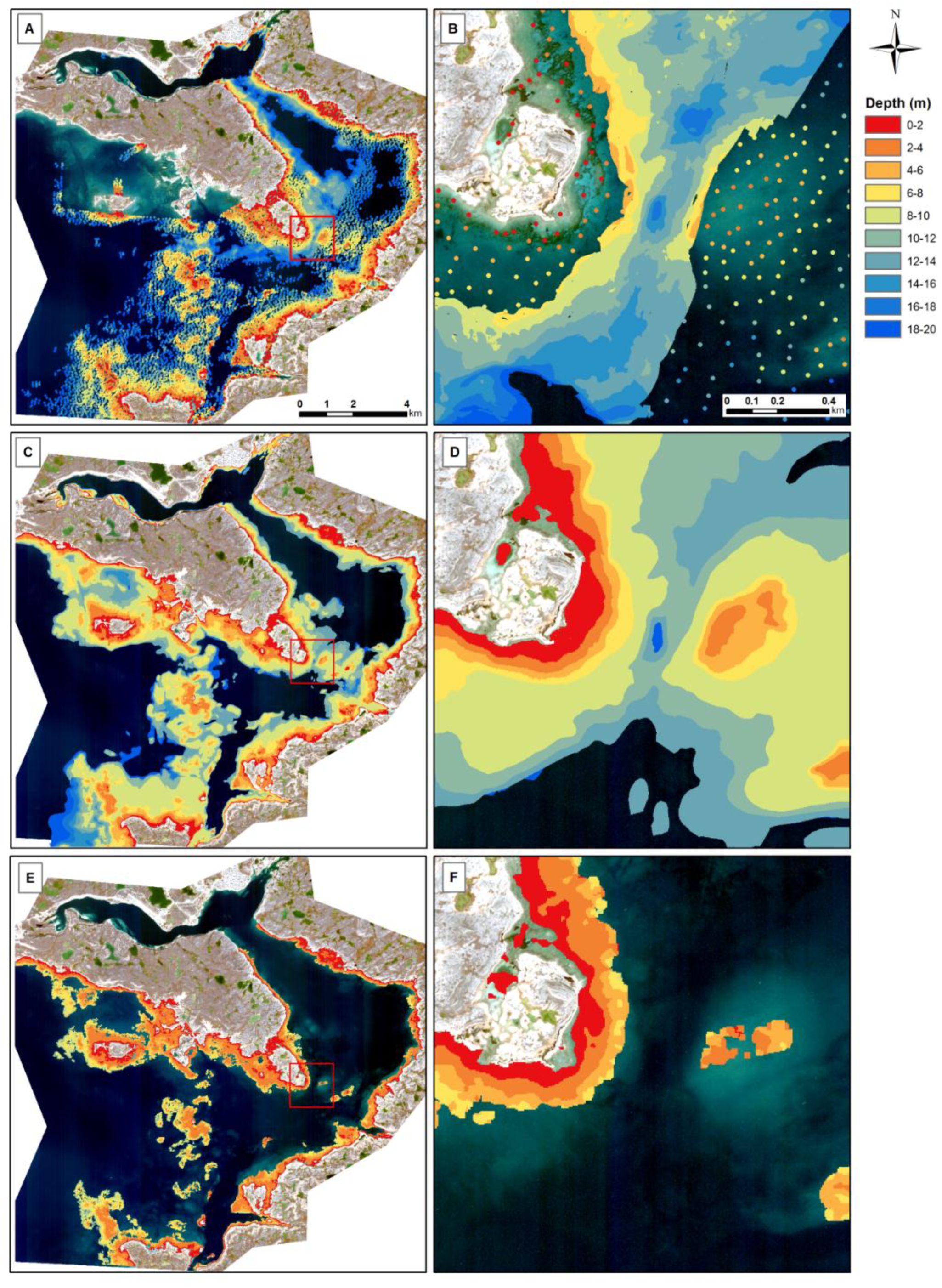
The analysis was divided into two main parts: (1) automatic extraction of a DSM for bathymetry, and (2) manual DSM extraction. This section presents a comparison of the DSM results obtained using both approaches.
Figure 4A,C present the bathymetry results from the automatic approach. Overall, this technique was able to identify 57% of the total 0–15 m depths (relative to survey data) present within the study site. The results were found to be poor in areas containing homogeneous seabed conditions, as the lack of variation between pixels within each image prevented accurate matching for the pair.
Figure 4B,D present the bathymetry results from the manual approach. This technique allowed depths to be extracted up to 20 m, an improvement over the automatic technique. The area covered by estimated depths was also greater for this result, as the technique is not subject to limitations with regard to homogeneous bottom areas.
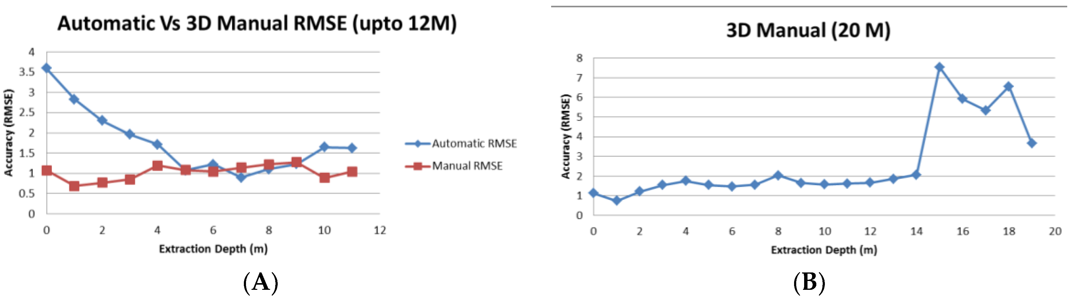
RMSE values calculated for the automatic and manual approaches (Figure 5A and Table 4) reveal that the manually extracted DSM showed an overall RMSE of ~1 m. The RMSE values calculated for depth ranges show the stability of the results across all depths for this approach, with a maximum RMSE of 1.88 m observed for depths of 8–10 m. In contrast, the automatically extracted DSM shows a high RMSE in shallow depths (0–4 m), with better results observed for greater depths. The 90% confidence levels were similar between the techniques, with 1.70 and 1.80 m observed for the manual and automatic approaches, respectively. Overall, the manual approach provided better accuracy for the majority of depths than the automatic approach.
The manual approach was further evaluated by considering all available survey points up to 20 m (Figure 5B). This revealed that depths up to 14 m obtained stable results with a low RMSE (>2 m); however, for deeper waters (>15 m), high error rates were found. These results suggest that the manual approach was able to reasonably determine depths up to 14 m.

5. Discussion

5.1. Survey Data Limitations

Further analysis of the survey data used for accuracy assessment identified a potential source of some of the high RMSE values identified in the results section. Table 5 presents the RMSE and bias statistics calculated between the surveys used for accuracy assessment. From the table, a high RMSE of ~1.30 m was identified between the LiDAR and overlapping multibeam surveys. This difference could be partially explained by the characteristics of these surveying techniques. Further, with 22–32 years between the acquisition of the LiDAR and multibeam data, the difference could also be explained by temporal changes due to sedimentation and erosion. An RMSE of 0.7 m observed between the 2014 and 2017 multibeam surveys also suggests an influence of temporal change.
Previous work completed by the CHS demonstrated that accuracies of ~1 m can be obtained using empirical SDB techniques [2,36]. As such, the potential reduced accuracy of some of the LiDAR data used within this analysis may be contributing significantly to the higher level of error observed for some of the stereo results. However, while not representing an ideal dataset, it remains important to include the LiDAR information in order to provide appropriate validation, particularly within shallow water (0–2 m) where multibeam survey information is limited.

5.2. Stereo Approach Comparisons

Advantages and disadvantages can be identified for both photogrammetric approaches. For the automatic approach, the main limitation is that image matching will not necessary work in all conditions. As an example, matching did not perform well over homogeneous seabed areas (e.g., sand) as it is impossible for pixels to be correlated between each image (Figure 6). Matching limitations resulted in a maximum depth of 12 m being obtained using the automatic approach, with many coverage gaps present within the 10–12 m depth range. The main advantage of the automatic approach is that DSMs can be completed quickly. After the completion of image pre-processing and the collection of tie points, the DSM can be extracted in less than one hour.
For the manual approach, the main advantage is that the technique is less sensitive to bottom type, allowing depth to be extracted for areas where the bottom is visible. The main disadvantages relate to the uncertainties inherent within manual techniques, as well as processing time. The quality of manually extracted DSMs will vary with the skill of the photogrammetrist. The approach is also more costly due to the significant time required for processing.
In order to benefit from the advantages of the manual and automatic approaches and to reduce the time required for the manual stereoscopic extraction, a first step could involve the use of the automatic approach to provide an initial estimate of depth. For locations where the automatic approach was unable to derive depth (e.g., due to homogenous bottom features), or where the uncertainties relative to survey depths are determined to be too great, the manual approach could be targeted to attempt to create a complete model.

5.3. International Standard Compatibility

Before being incorporated into nautical products, bathymetric information has to be evaluated against International Hydrographic Organization (IHO) standards. The IHO accuracy requirements for surveys are defined within the IHO S-57 standard [37], specifically through CATZOC levels. Table 6 provides an overview of the CATZOC requirements for hydrographic surveys. The positional accuracy of high-resolution optical imagery, such as that provided by WorldView-2, allows satellite data to meet the CATZOC A level. However, the level of uncertainty present within the results of the photogrammetric techniques prevents a CATZOC A classification for depth accuracy. As such, the CHS would likely classify the results of the photogrammetric technique as CATZOC C. While possible in theory, significant discussion remains to be completed within the CHS, as well as amongst international hydrographic offices, in order to determine the appropriate CATZOC classifications for satellite-derived depth information.

6. Conclusions

This study explored the potential of two photogrammetric techniques (automatic and 3D manual) for deriving estimates of depth within Canadian waters. Using a WorldView-2 image acquired over Cambridge Bay, Nunavut, DSMs were generated using each technique, resulting in depths being estimated accurately up to ~15 m.
An accuracy assessment completed using in situ CHS survey data showed that both approaches have the potential to estimate depth with ~1 m of error for some ranges of depth, meeting the IHO’s CATZOC C level for survey quality. In general, the 3D manual photogrammetric technique performed better than the automatic approach, achieving RMSEs of no more than 1.88 m for depths up to 12 m. However, with depths > 15 m, the manual approach was found to perform poorly, with RMSEs of more than 7 m observed for these larger depths.
While the results show the potential of both approaches for estimating depth in Canadian waters, neither technique appears to represent an ideal, single solution for estimating depth. The automatic approach, while simple and quick to apply, resulted in large uncertainties for shallow waters, limiting its effectiveness. In contrast, while the manual approach allowed depth to be estimated up to ~20 m, it contained significant errors with greater depth. The nature of the 3D manual approach also increases its costs, limiting its potential for wide area applications. Overall, a combined approach, using the advantages of each technique, may be preferred. For example, the automatic technique could initially be applied to derive depth over as many areas as possible. The 3D manual technique could then be applied to extend estimates to deeper waters and to remove gaps within the automatically extracted depths (e.g., over homogeneous depth areas).
The application of such a hybrid approach, as well as a potential combination with reflectance-based SDB techniques, presents a promising approach for gaining a more representative understanding of depth within Canadian coastal waters. Stereo photogrammetric approaches are particularly promising for application in Arctic waters, where a lack of available in situ survey data presents limitations for empirical SDB techniques. Through future work, the CHS aims to identify best practices for stereo and other bathymetry estimation techniques in order to advance the use of satellite information within navigational products.

Author Contributions

Conceptualization, methodology, supervision, project administration and funding acquisition, R.C.; formal analysis, investigation and validation, Y.S. and M.S.; Writing—original draft preparation, R.C., Y.S., M.S., M.-A.F., and R.A.; and writing—review & editing, R.C., M.-A.F., R.A., and M.S.

Funding

The CHS received support through the Canadian Space Agency’s Government Related Initiatives Program to complete this work.

Acknowledgments

Special thanks to Matus Hodul, a M.Sc. graduate from the University of Ottawa, who worked at the CHS during his studies and helped in the development of the automatic photogrammetric extraction process used in this study. Thanks to Loretta Abado for her help in the review and editing of the article. The extraction of the isobaths for the manual photogrammetric approach was completed under a contract with Effigis Geo Solutions.

Conflicts of Interest

The authors declare no conflict of interest. The funders had no role in the design of the study; in the collection, analyses, or interpretation of data; in the writing of the manuscript, or in the decision to publish the results.

References

  1. Department of Fisheries and Oceans (DFO). The Role of the Canadian Government in the Oceans Sector. 2008. Available online: http://www.dfo-mpo.gc.ca/oceans/publications/cg-gc/page02-eng.html (accessed on 22 June 2018).
  2. Chenier, R.; Faucher, M.A.; Ahola, R.; Jiao, X.; Tardif, L. Remote sensing approach for updating CHS charts. In Proceedings of the Canadian Hydrographic Conference, Halifax, NS, Canada, 16–17 May 2016. [Google Scholar]
  3. Polcyn, F.C.; Brown, W.L.; Sattinger, I.J. The Measurement of Water Depth by Remote Sensing Techniques; Report No. 8973-26-F; Willow Run Laboratories of the Institute of Science and Technology, the University of Michigan: Ann Arbor, MI, USA, 1970. [Google Scholar]
  4. Lyzenga, D.R. Passive remote sensing techniques for mapping water depth and bottom features. Appl. Opt. 1978, 17, 379–383. [Google Scholar] [CrossRef] [PubMed]
  5. Lyzenga, D.R. Remote sensing of bottom reflectance and water attenuation parameters in shallow water using aircraft and LANDSAT data. Int. J. Remote Sens. 1981, 2, 71–82. [Google Scholar] [CrossRef]
  6. Lyzenga, D.R. Shallow-water bathymetry using combined LiDAR and passive multispectral scanner data. Int. J. Remote Sens. 1985, 6, 115–125. [Google Scholar] [CrossRef]
  7. Lee, Z.; Carder, K.L.; Mobley, C.D.; Steward, R.G.; Patch, J.S. Hyperspectral remote sensing for shallow waters: 2. Deriving bottom depths and water properties by optimization. Appl. Opt. 1999, 38, 3831–3843. [Google Scholar] [CrossRef] [PubMed]
  8. Stumpf, R.P.; Holderied, K.; Sinclair, M. Determination of water depth with high-resolution imagery over variable bottom types. Limnol. Oceanogr. 2003, 48, 547–556. [Google Scholar] [CrossRef]
  9. Knudby, A.; Ahmad, S.K.; Ilori, C. The potential for landsat based bathymetry in Canada. Can. J. Remote Sens. 2016, 367–378. [Google Scholar] [CrossRef]
  10. Kerr, J.M.; Purkis, S. An algorithm for optically-deriving water depth from multispectral imagery in coral reef landscapes in the absence of ground-truth data. Remote Sens. Environ. 2018, 210, 307–324. [Google Scholar] [CrossRef]
  11. Mavraeidopoulos, A.K.; Pallikaris, A.; Oikonomou, E. Satellite derived bathymetry (SDB) and safety of navigation. Int. Hydrogr. Rev. 2017, 7–19. Available online: https://journals.lib.unb.ca/index.php/ihr/article/download/26290/1882519043 (accessed on 25 July 2018).
  12. Dean, R.G.; Dalrymple, R.A. Water wave mechanics for engineers and scientists. Adv. Ser. Ocean Eng. 1991. [Google Scholar] [CrossRef]
  13. Alpers, W.; Hennings, I. A theory of the imaging mechanism of underwater bottom topography by real and synthetic aperture radar. J. Geophys. Res. 1984, 89, 10529–10546. [Google Scholar] [CrossRef]
  14. Pleskachevsky, A.; Lehner, S. Estimation of Underwater Topography Using Satellite High Resolution Synthetic Aperture Radar Data. 2011. Available online: https://www.researchgate.net/publication/225023003/download (accessed on 5 September 2018).
  15. Danilo, C.; Melgani, F. Wave period and coastal bathymetry using wave propagation on optical images. IEEE Trans. Geosci. Remote Sens. 2016, 54, 6307–6319. [Google Scholar] [CrossRef]
  16. Li, X.; Yang, X.; Zheng, Q.; Pietrafesa, L.J.; Pichel, W.G.; Li, Z.; Li, X. Deep-water bathymetric features imaged by spaceborne SAR in the Gulf Stream region. Geophys. Res. Lett. 2010, 37. [Google Scholar] [CrossRef] [Green Version]
  17. Mancini, S.; Olsen, R.C.; Abileah, R.; Lee, K.R. Automating nearshore bathymetry extraction from wave motion in satellite optical imagery. In Proceedings of the SPIE Defense, Security, and Sensing, Baltimore, MD, USA, 23–27 April 2012. [Google Scholar]
  18. Fujisada, H.; Urai, M.; Iwasaki, A. Technical methodology for ASTER global DEM. IEEE Trans. Geosci. Remote Sens. 2012, 50, 3725–3736. [Google Scholar] [CrossRef]
  19. Hodul, M.; Bird, S.; Knudby, A.; Chenier, R. Satellite derived photogrammetric bathymetry. ISPRS J. Photogramm. Remote Sens. 2018, 142, 268–277. [Google Scholar] [CrossRef]
  20. Li, R.; Zhou, F.; Niu, X.; Di, K. Integration of Ikonos and QuickBird imagery for geopositioning accuracy analysis. Photogramm. Eng. Remote Sens. 2007, 73, 1067–1074. [Google Scholar]
  21. Li, R.; Niu, X.; Liu, C.; Wu, B.; Deshapnde, S. Impact of imaging geometry on 3D geopositioning accuracy of stereo Ikonos imagery. Photogramm. Eng. Remote Sens. 2009, 75, 1119–1125. [Google Scholar] [CrossRef]
  22. Jeong, J.; Kim, T. Analysis of dual-sensor stereo geometry and its positioning accuracy. Photogramm. Eng. Remote Sens. 2014, 80, 653–661. [Google Scholar] [CrossRef]
  23. Jeong, J.; Kim, T. Quantitative estimation and validation of the effects of the convergence, bisector elevation, and asymmetry angles on the positioning accuracies of satellite stereo pairs. Photogramm. Eng. Remote Sens. 2016, 82, 625–633. [Google Scholar] [CrossRef]
  24. Cain, J. Stereomodel Acquisition Geometry. Ph.D. Thesis, University of California, Berkley, CA, USA, 1989. [Google Scholar]
  25. Tong, X.; Liu, S.; Weng, Q. Bias-corrected rational polynomial coefficients for high accuracy geo-positioning of QuickBird stereo imagery. ISPRS J. Photogramm. Remote Sens. 2010, 65, 218–226. [Google Scholar] [CrossRef]
  26. Hedley, J.D.; Harborne, A.R.; Mumby, P.J. Simple and robust removal of sun glint for mapping shallow-water benthos. Int. J. Remote Sens. 2005, 26, 2107–2112. [Google Scholar] [CrossRef]
  27. Helava, U.V. Digital correlation in photogrammehic instruments. Photogrammetria 1978, 34, 19–41. [Google Scholar] [CrossRef]
  28. Bulatov, D.; Wernerus, P.; Heipke, C. Multi-view dense matching supported by triangular meshes. ISPRS J. Photogramm. Remote Sens. 2011, 66, 907–918. [Google Scholar] [CrossRef]
  29. Harwin, S.; Lucieer, A. Assessing the accuracy of georeferenced point clouds produced via multi-view stereopsis from unmanned aerial vehicle (UAV) imagery. Remote Sens. 2012, 4, 1573–1599. [Google Scholar] [CrossRef]
  30. Knapitsch, A.; Park, J.; Zhou, Q.; Koltun, V. Tanks and temples: Benchmarking large-scale scene reconstruction. ACM Trans. Graph. 2017. [Google Scholar] [CrossRef]
  31. Hirschmüller, H. Accurate and efficient stereo processing by semi-global matching and mutual information. In Proceedings of the 2005 IEEE Computer Society Conference on Computer Vision and Pattern Recognition, San Diego, CA, USA, 20–25 June 2005; pp. 807–814. [Google Scholar]
  32. Hirschmuller, H. Stereo processing by Semi-Global Matching and Mutual Information. IEEE Trans. Pattern. Anal. Mach. Intell. 2008, 30, 1–14. [Google Scholar] [CrossRef] [PubMed]
  33. Pairaud, I.L.; Lyard, F.; Auclair, F.; Letellier, T.; Marsalaix, P. Dynamics of the semi-diurnal and quarter-diurnal internal tides in the Bay of Biscay. Part 1: Barotropic tides. Cont. Shelf Res. 2008, 28, 1294–1315. [Google Scholar] [CrossRef]
  34. Collins, A.K.; Hannah, C.G.; Greenberg, D. Validation of a high resolution modelling system for tides in the Canadian Arctic archipelago. Candian Technical Report of Hydrography and Ocean Sciences. 2011. Available online: http://www.dfo-mpo.gc.ca/Library/343683.pdf (accessed on 25 July 2018).
  35. Murase, T.; Tanaka, M.; Tani, T.; Mayashita, Y.; Ohkawa, N.; Ishiguro, S.; Suzuki, Y.; Kayanne, H.; Yamano, H. A photogrammetric correction procedure for light refraction effects at a two-medium boundary. Photogramm. Eng. Remote Sens. 2008, 74, 1129–1136. [Google Scholar] [CrossRef]
  36. Chénier, R.; Faucher, M.-A.; Ahola, R. Satellite-derived bathymetry for improving Canadian Hydrographic Service charts. ISPRS Int. J. Geo-Inf. 2018, 7, 306. [Google Scholar] [CrossRef]
  37. International Hydrographic Organization (IHO). S-57 Supplement No. 3—Supplementary Information for the Encoding of S-57 Edition 3.1 ENC Data; International Hydrographic Organization: Monaco, Monaco, 2017; Available online: https://www.iho.int/iho_pubs/standard/S-57Ed3.1/S-57_e3.1_Supp3_Jun14_EN.pdf (accessed on 5 June 2018).
Figure 1. Cambridge Bay study area located in the Canadian Arctic on Victoria Island, Nunavut. Background map © ESRI.
Ijgi 07 00395 g001
Figure 2. (A) Distribution of multibeam survey data (2014, 2015 and 2017) and LiDAR surveys (1985, 1992) over the study site. (B) Hydrographic survey data of ≤ 20 m water depth used for accuracy assessment. Imagery © 2015, DigitalGlobe, Inc.
Ijgi 07 00395 g002
Figure 3. WordView-2 stereo-pair acquired on 20 September 2015: (A) forward image, (B) backward image. Imagery © 2015, DigitalGlobe, Inc.
Ijgi 07 00395 g003
Figure 4. Comparisons between CHS survey data and stereo photogrammetry approaches for the entire WorldView-2 image and an inset area. (A,B): CHS survey data. (C,D): manual approach results. (E,F): automatic approach results. All share the same colour scheme shown in the legend. Imagery © 2015, DigitalGlobe, Inc.
Ijgi 07 00395 g004
Figure 5. (A) Evaluation of the RMSE calculated for the automatic and manually extracted DSMs (up to 12 m) using overlapping survey points. (B) RMSE for the manually extracted DSM up to 20 m using all survey points.
Ijgi 07 00395 g005
Figure 6. Impact of homogenous bottom types on the automatic approach. (A) Homogeneous areas within the WorldView-2 image. (B) Illustration of gaps in bathymetry estimates from the automatic approach due to areas of homogeneous bottom.
Ijgi 07 00395 g006
Table 1. CHS hydrographic surveys used within this study.
Survey TypeDate of AcquisitionCATZOC ClassificationNumber of Points (0–20 m)
Multibeam1 August to 10 September 2017A1599,305
1 August to 30 September 2015A11,265,263
6 August to 19 September 2014A11,284,582
LiDAR1–31 August 1992C1193
1–31 August 1985B8953
Total 3,159,297
Table 2. Distribution of survey points for water depth ranges.
Water Depth (m)2017 Multibeam2015 Multibeam2014 Multibeam1992 LiDAR1985 LiDARTotal
0 to 2009382597331930
2 to 4044010,16324592711,775
4 to 6167117,75346,308200106066,992
6 to 815,05257,95782,5741341052156,769
8 to 1023,380120,681104,9281241105250,218
10 to 1267,570199,580166,65948724434,581
12 to 14150,157270,770211,43354891633,305
14 to 16137,498189,464202,00133816529,812
16 to 18140,050228,040243,40442813612,349
18 to 2063,927180,578216,17454825461,558
Total599,3051,265,2631,284,582119389463,159,289
Table 3. Image and stereo-pair geometry.
Image GeometryForward ImageBackward ImageStereo GeometryStereo-Pair
In-Track View24°−8°Convergence36.3°
Cross Track View14.7°14.1°BIE71.2°
Off Nadir View28°16.2°Asymmetrical9.5°
Table 4. RMSEs and 90% confidence levels for automatic and manual approaches.
AutomaticManual
Depth Range90% Conf. LevelRMSE (m)Bias (m)Min Error (m)Max Error (m)90% Conf. LevelRMSE (m)Bias (m)Min Error (m)Max Error (m)
0–10 m1.841.460.840.0012.511.701.17−0.470.006.80
0–2 m 3.131.840.0012.51 1.090.610.003.20
2–4 m 2.071.610.005.68 1.12−0.160.003.85
4–6 m 1.400.880.006.13 1.28−0.520.004.10
6–8 m 1.120.530.008.50 1.57−0.410.004.80
8–10 m 1.140.230.004.78 1.88−0.210.006.80
10–12 m 1.651.060.003.70 0.900.180.004.57
Table 5. RMSE and bias between the CHS surveys for Cambridge Bay.
2015–20142017–20142017–2015Lidar-MB
Count118,195152,46099,2431758
RMSE0.200.670.291.30
Bias−0.18−0.46−0.270.60
Table 6. IHO CATZOC specifications [37].
CATZOC TypeHorizontal AccuracyVertical Accuracies for Depth RangesSeafloor Coverage
Depth Range (m)Accuracy
A15 m0–10±0.6Full coverage
10–30±0.8
A220 m0–10±1.2Full coverage
10–30±1.6
B50 m0–10±1.2Full coverage not achieved, hazards to surface navigation are not expected but may exist
10–30±1.6
C500 m0–10±2.5Full coverage not achieved, depth anomalies may be expected
10–30±3.5

