Article

CO-RIP: A Riparian Vegetation and Corridor Extent Dataset for Colorado River Basin Streams and Rivers

1
Natural Resource Ecology Laboratory, Colorado State University, Fort Collins, CO 80523, USA
2
Graduate Degree Program in Ecology, Colorado State University, Fort Collins, CO 80523, USA
3
NASA DEVELOP Colorado Center, Fort Collins, CO 80523, USA
4
Department of Earth and Planetary Sciences, John Hopkins University, Baltimore, MD 21218, USA
5
US Geological Survey, Fort Collins Science Center, Fort Collins, CO 80523, USA
*
Author to whom correspondence should be addressed.
ISPRS Int. J. Geo-Inf. 2018, 7(10), 397; https://0-doi-org.brum.beds.ac.uk/10.3390/ijgi7100397
Submission received: 18 July 2018 / Revised: 28 August 2018 / Accepted: 22 September 2018 / Published: 5 October 2018

Abstract

:
Here we present “CO-RIP”, a novel spatial dataset delineating riparian corridors and riparian vegetation along large streams and rivers in the United States (US) portion of the Colorado River Basin. The consistent delineation of riparian areas across large areas using remote sensing has been a historically complicated process partially due to differing definitions in the scientific and management communities regarding what a “riparian corridor” or “riparian vegetation” represents. We use valley-bottoms to define the riparian corridor and establish a riparian vegetation definition interpretable from aerial imagery for efficient, consistent, and broad-scale mapping. Riparian vegetation presence and absence data were collected using a systematic, flexible image interpretation process applicable wherever high resolution imagery is available. We implemented a two-step approach using existing valley bottom delineation methods and random forests classification models that integrate Landsat spectral information to delineate riparian corridors and vegetation across the 12 ecoregions of the Colorado River Basin. Riparian vegetation model accuracy was generally strong (median kappa of 0.80), however it varied across ecoregions (kappa range of 0.42–0.90). We offer suggestions for improvement in our current image interpretation and modelling frameworks, particularly encouraging additional research in mapping riparian vegetation in moist coniferous forest and deep canyon environments. The CO-RIP dataset created through this research is publicly available and can be utilized in a wide range of ecological applications.

1. Introduction

The Colorado River is one of the most important water resources for people, wildlife, and agriculture in the southwestern United States (U.S). Its headwaters begin at 2743 m a.s.l. at La Poudre Pass in Colorado and, under natural flow regimes, empties into the Gulf of California 2333 km downstream. Ephemeral, seasonal, and persistent riparian habitats are found throughout the Colorado River Basin, which hosts some of the most important vegetative communities for wildlife species in the predominantly arid landscape [1]. Riparian corridors are associated with numerous ecosystem services, including water and sediment flow dynamics [2,3], water quality [3], habitat, forage and fiber for wildlife, maintenance of biodiversity [3,4], and recreation and aesthetics [4]. Riparian areas have rich floral and faunal diversity [2], with many terrestrial animal species reliant on riparian corridors [4] for the provisioning of food, water, shelter, and corridors for species migration [4,5,6,7]. Still, riparian areas represent a relatively small percentage of the total land cover of the western US [4], are intensively disturbed [2,8], and are often considered to be at-risk ecosystems in semi-arid regions [4,9] due to the effects of urbanization [10], agriculture [11], and modified water flow regimes [12]. The spatial distribution of riparian areas is often inconsistently reported, as defining the extent of a riparian corridor or determining what composes riparian versus non-riparian vegetation remains an ongoing debate. Currently, there is no universal definition of “riparian vegetation” or a “riparian corridor.” Riparian vegetation is only vaguely represented at the landscape scale in existing US land cover datasets, such as the National Land Cover Database [13,14] and LANDFIRE existing vegetation layers [15].
The need to create and improve upon existing riparian area datasets has been shown to be a key scientific management priority with the creation of US based initiatives to improve mapping of riparian vegetation types, such as that occurring in the Southwest ReGAP Program [16] in the United States and in international initiatives, such as the Copernicus Program’s “Riparian Zones” [17] layer in Europe. In the United States, a paucity of explicit information on the location and extent of riparian corridors remains, partially because existing datasets do not include hydro-geomorphological data, such as the extent of valley bottoms, to delineate riparian cover [4,15]. A detailed map of riparian corridors is expressly needed in the Colorado River Basin, where the social-ecological significance and the increasing vulnerability of riparian systems have led to several management and conservation initiatives. Two examples include The Nature Conservancy’s Colorado River Program, which manages 15 restoration and conservation projects in the basin, and the Bureau of Reclamation’s Lower Colorado River Multi-Species Conservation Program (LCR-MSCP), which manages riparian habitat for the recovery of listed species including the endangered Southwestern willow flycatcher (Empidonax traillii extimus) [18,19,20]. Comprehensive information concerning the location and extent of riparian vegetation can support these and similar habitat conservation and management actions across the basin.
At local and regional scales, riparian corridors are delineated in numerous ways, as their definition is usually dependent on research approach or agency targets. Generally, they are the transition between terrestrial and freshwater ecosystems [2,21,22] and include components of topography, vegetation, and soils. Riparian corridors are dynamic regions with complex heterogenic landscapes formed by frequent disturbances [23], and therefore, are challenging to delineate and map across large spatial scales [4,24,25,26]. Even fixed buffers along streams have been broadly employed in delineating riparian corridors. The total potential maximum extent of riparian corridors can be captured based on geomorphology [27], and within this area, temporal fluctuations in riparian corridor vegetation can be evaluated with spectral imagery [24,27]. In many areas, riparian vegetation is spectrally inimitable because of its more persistent greenness when compared to upland areas and other landcover classes [28]. Here, we use topography to define the boundaries of the riparian corridor and use spectral remote sensing to differentiate non-riparian vegetation and landscape features from riparian vegetation within these corridors.
The goal of this study was to create “CO-RIP”, a publicly available dataset of riparian vegetation and riparian corridors along the US portion of the Colorado River and its major tributaries. To achieve this goal, this study had the following objectives: (1) Delineate the maximum extent of the riparian corridor as defined by topographic features, (2) use remote sensing to detect riparian vegetation, and (3) integrate these products to create a cumulative riparian extent and vegetation dataset for the major streams and rivers in the Colorado River Basin. In addition to producing the highest spatial resolution riparian corridor and vegetation dataset available for the Colorado River Basin, this research provides a new framework for defining riparian vegetation in the context of remote sensing and integrates two existing methodologies (valley bottom delineation and spectral remote sensing of vegetation) into a single, process based framework that can be employed to delineate riparian corridors and vegetation in regions across the globe.

2. Materials and Methods
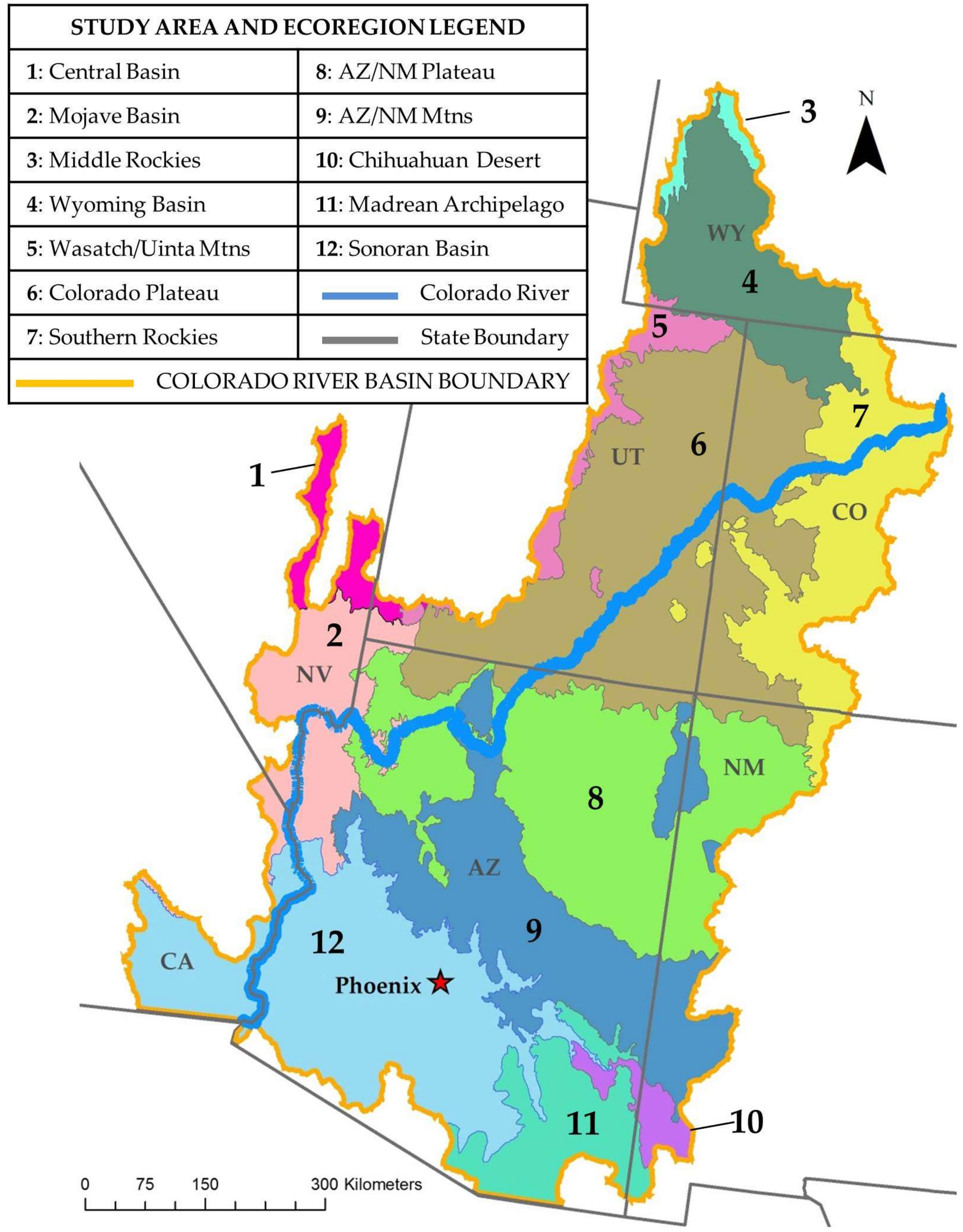
2.1. Study Area

The study area encompassed the entirety of the US portion of the Colorado River Basin, an extensive and ecologically diverse watershed that covers 637,000 km2 over seven states, including Colorado, Wyoming, New Mexico, Arizona, Utah, Nevada, and California (Figure 1). The Colorado River Basin stretches longitudinally over 2300 km and is characterized by its intense topographic diversity, with elevations ranging from sea level at the Gulf of California to over 4000 m in the highest areas of the Rocky Mountains of Colorado. The basin’s complex network of streams and rivers drain into the Colorado River, one of the largest rivers by length and drainage area in the United States [29]. The river and its basin are characterized by twelve different ecologically distinct regions ([30], Appendix A) and dominated by four (Figure 1).
Coniferous forests and alpine meadow environments characterize the River’s mountainous headwaters, where the Colorado River is relatively small and primarily fed by seasonal snowpack. Further southward, the Arizona and New Mexico Plateau and Mountains are characterized by dense coniferous forests at high elevations, pinyon (Pinus spp.) and juniper (Juniperus spp.) forests at mid-elevations and sagebrush (Artemisia spp.) and chaparral in lower elevation areas where precipitation is low, resulting in a dry, arid environment. The Colorado River flows through the Grand Canyon in Arizona, into the dry, sparsely vegetated semi desert and desert environments flanking much of the southern basin. In its final stretch, the river travels through the Sonoran Basin and Range, encompassing a portion of northern Mexico, passing through arid, desert environments where saguaro (Carnegiea gigantean) and cholla cactus (Cylindropuntia spp.) and creosote bush (Larrea tridentate) dominate the landscape [30]. A detailed description of each ecoregion, modified from [30], is provided in Appendix A.

2.2. Mapping Valley Bottoms a Proxy for the “Riparian Corridor Extent”

Riparian areas are shaped and bounded by the same topographic and hydrologic processes that define the topography of valley bottoms. Valley bottoms are therefore representative of the “maximum riparian corridor extent” [31,32,33], an area which separates the vegetative, topographic, and environmental characteristics of riparian areas from those of the upland (hereafter, the “maximum riparian corridor extent” will be referred to as “riparian corridor”). We used the Valley Bottom Extraction Tool (V-BET) [33], a freely available ArcMap Toolbox [34], to map valley bottoms as a proxy for the riparian corridor across the Colorado River Basin. The V-BET tool allows for efficient delineation of valley bottoms across larger spatial extents and at higher resolutions than has typically been possible with publicly available datasets in the past [33]. We applied the V-BET algorithm to all streams and rivers present within the Colorado River Basin that were greater than or equal to Strahler stream order “3” [35], thereby capturing the extent of riparian corridors along the majority of large streams and rivers within the Colorado River Basin.
The V-BET tool’s derivative inputs can be obtained from two primary data sources: A high resolution (10 m2 or less) digital elevation model (DEM) and hydrologic flowline data with high cartographic precision. We obtained a 10 m2 digital elevation model from the National Elevation Dataset [36] and a hydrologic flow line data from the National Hydrography Dataset (NHD) [37]. Flowlines representing ephemeral streams, storm water infrastructure, pipelines, canals, and aqueducts were removed as well as the NHD dataset’s ‘artificial paths’ within lakes and waterbodies with an area greater than 0.0005 km2. If there were sinks present within the DEM they were filled to remove local depressions, and then slope, aspect, flow direction, flow accumulation and drainage area rasters were created from the DEM as derivative inputs to V-BET. To maintain processing efficiency, we separated the study area using hydrological unit codes (HUCs) at the HUC-6 level [38] and processed each HUC independently within the V-BET toolbox in ArcMap v10.3 [34]. Resulting valley bottom extents, which are output from the tool as polygon files, were qualitatively verified by trained interpreters and edited manually in a geographic information system (GIS) to remove any superfluous channels or over/under estimations of extent using the refinement and editing process detailed in reference [33]. Due to the absence of field measurements, large size of the study area, and the lack of a standardized measure of valley bottomness, an accuracy assessment of the resulting valley bottom extents was conducted qualitatively using ancillary data sources [33], including high resolution (1 m2) National Agriculture Imagery Program (NAIP) imagery, hill shade, and slope rasters in conjunction with ocular validation.

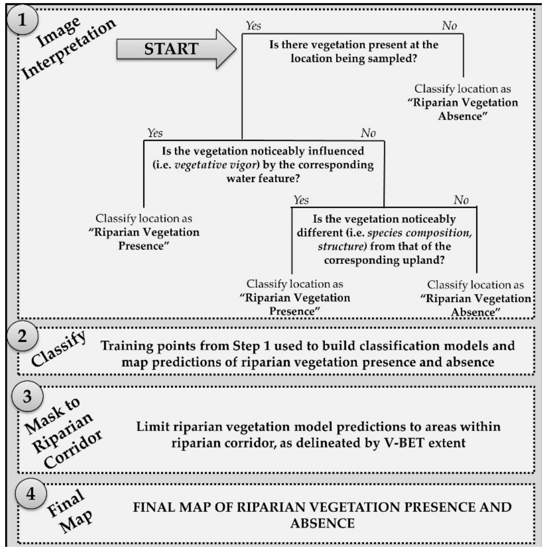
2.3. Mapping Riparian Vegetation

Our valley bottom analyses delineated the extent of the riparian corridor by land area, but a secondary analysis was necessary to determine the extent and cover of riparian vegetation within delineated valley bottoms. Due to the large spatial extent of the study area and the need to collect historical training samples for classification models, digital image sampling was used to collect environmental response data. Trained image interpreters used high resolution NAIP imagery for 2016 to ocularly interpret the presence and absence of riparian vegetation within the edited valley bottom extents. NAIP imagery is collected either biannually or on a 3 year rotating cycle, with some states in the Colorado River Basin collected in even years and others during odd years, so imagery was selected as close to the focal year of 2016 as possible (± 1 year). Where 4-band NAIP imagery was available, interpreters also used false color band combinations that helped to highlight the presence of vegetation.
We separated our digital image sampling into 12 distinct ecoregions using the Environmental Protection Agency (EPA) Level III ecoregion product [39] to reduce vegetative and environmental variability within the training data. Using a scripted Google Earth Engine image visualization and data collection interface [34], riparian vegetation presence and absence training points were collected in each ecoregion in a purposive fashion [40]. We used purposive sampling to integrate the expert opinion of the interpreter in the selection and distribution of our sampling locations. This helps to ensure sampled locations represented the full range of environmental and spectral variability present on the landscape. Riparian vegetation presence points had to meet multiple criteria (Figure 2) to be classified as riparian vegetation: (1) The location sampled had vegetation present and (2) the vegetation at that location was either visually assessed to be influenced by the corresponding water feature [41,42], or the vegetation was noticeably unique from that of the upland with regard to species composition, structure, or vegetative vigor. Riparian vegetation absence points were defined as locations within the valley bottom where riparian vegetation is not present (i.e., bare ground, rock, structures) or locations where vegetation is present at the location in the valley bottom but was not characteristic of riparian vegetation (e.g., agricultural areas or vegetation located in the valley bottom that could not be differentiated from those observed in upland areas). Sampling points were placed in areas where the classification type dominated the immediate area, with care taken so that points were not placed on the edge of multiple classification types (i.e., points were placed in the middle of a riparian vegetation clump instead of on the edge of a vegetation-bare soil gradient). We collected hundreds of training samples in each ecoregion so that a range of vegetative densities would be represented (Appendix B).
Interpreters intentionally placed points to represent the diversity of riparian and non-riparian vegetation, including in areas where agriculture had multiple spectral signals/gradients. Training data locations were spaced sufficiently to prevent double sampling of a pixel in Landsat imagery, which has a spatial resolution of 30 × 30 m. In total, we collected 6672 presence samples and 7839 absence samples across the Colorado River Basin. These samples are further summarized by each ecoregion in Appendix B.
To create spectral predictors of riparian vegetation, we composited Landsat 8 Operational Land Imager (OLI) imagery for 2016 using the median pixel values of all available cloud-free image collections from a two month period in the growing season (1 July–31 August). Median pixel value images from the growing season were selected to represent leaf-on riparian vegetation in a pre-senescent state. Additional spectral indices were then created using these composited image products including the tasseled cap transformation [43] specifically created for Landsat 8 OLI [44], normalized difference vegetation index [45], Soil Adjusted Vegetation Index (SAVI) [46] and Modified Normalized Difference Water Index (mNDWI) [47]. In total, we selected eight Landsat bands corrected to top of atmosphere reflectance, four spectral indices, and two topographic surface rasters derived from the DEM as potential predictor variables (Table 1). We extracted predictor variable values from all rasters that corresponded with each of the recorded riparian presence/absence locations in preparation for our classification analyses.
We fit a unique random forests classification model [48] for each of the twelve ecoregions using the riparian vegetation training samples as the response and extracted predictor values. Random forests is a decision tree based classification algorithm that is beneficial for use in remote sensing analyses, as it is non-parametric, simple to evaluate and difficult to overfit [49]. A detailed description of the operation and evaluation of random forests is presented in reference [48] and a detailed description of the application of the algorithm for classification of landcover is offered in reference [50]. In an effort to balance computational power and efficiency, each random forests model was built with 1000 trees, with all other algorithmic tuning parameters left at the R Package Random forest’s default settings. Riparian vegetation was modelled at the EPA ecoregion level [39]. While there remains environmental heterogeneity within EPA ecoregions, this delineation was carried out to ensure models performed suitably across all riparian environments in the Colorado River Basin, which may have substantially varied spectral signatures from region to region.
We selected final combinations of model predictors using rfUtilities [51], a model selection package available in Program R v3.3 [52] that was created specifically for random forests. rfUtilities’ “rf.modelSel” function implements a model selection approach created in reference [53], which identifies the most parsimonious model by selecting the smallest combination of predictors with the highest pseudo-R2 and lowest mean squared error [53,54]. A covariate correlation plot was generated to remove correlated predictors and rfUtilities was used to generate variable importance. These two procedures were used together to determine the final set of predictors. We removed variables with less than 5% importance in the initial model selection. In the remaining set of covariates, if two variables were correlated above 0.8, only the variable with greater relative importance was kept. Removing correlated predictor variables enables clearer interpretation of variable importance values and can improve model performance [55]. We subsequently evaluated each model individually using out-of-bag metrics [48] and a 10-fold cross validation approach [56] to calculate error rates and kappa values. We additionally reported the percent contribution of each predictor in each final model and out of bag and cross-validated error, confusion matrices, class errors, as well as user’s and producer’s accuracies for each individual model (Appendix C). Given the size of our study area, on-the-ground field validation of our results was not possible, but we believe these standardly employed model evaluation approaches offer an accurate representation of model performance. Our final models were applied using our predictive raster surfaces to generate spatial predictions of the presence and absence of riparian vegetation across the Colorado River Basin, which was clipped to the V-BET extent.

3. Results

3.1. Valley Bottom/Maximum Riparian Corridor Extent Delineation

Our final valley bottom extent results produced using V-BET are available as polygons (Figure 3). The final results from the V-BET algorithm serve as our definition of the riparian corridor, but are not limited to this application and are distributed independently of our riparian vegetation layer for use in related analyses.
Substantial visual validation and manual editing was carried out by trained interpreters to correct any VBET extent errors that were observed in the results. Manual editing and validation was extensive, and took multiple interpreters a total of 320 h to complete. The majority of the errors occurred within two main environments: (1) Flatter floodplain areas and (2) high-elevation or high relief headwater regions. The flatter floodplain errors were most evident in the southern portion of the study area, primarily the Sonoran Basin and Mojave Basin. In contrast, the model errors which were observed in northern ecoregions, such as the southern Rockies, primarily occurred in locations displaying steep slopes. Valley bottom delineation errors likely occurred as a result of the 10 m2 digital elevation model used to delineate valley bottoms. While a 10 m2 digital elevation model is considered to be high resolution in many research settings, limitations remain in areas with steep slopes or narrow channels where an even higher spatial resolution DEM would be required to improve delineation accuracy. Depending on the width of the valley bottom and slope of surrounding features, valley bottoms could be both over or underestimated. Our errors are consistent with the observations seen in reference [33], which describes the reasoning for errors in V-BET outputs and provides detailed examples.

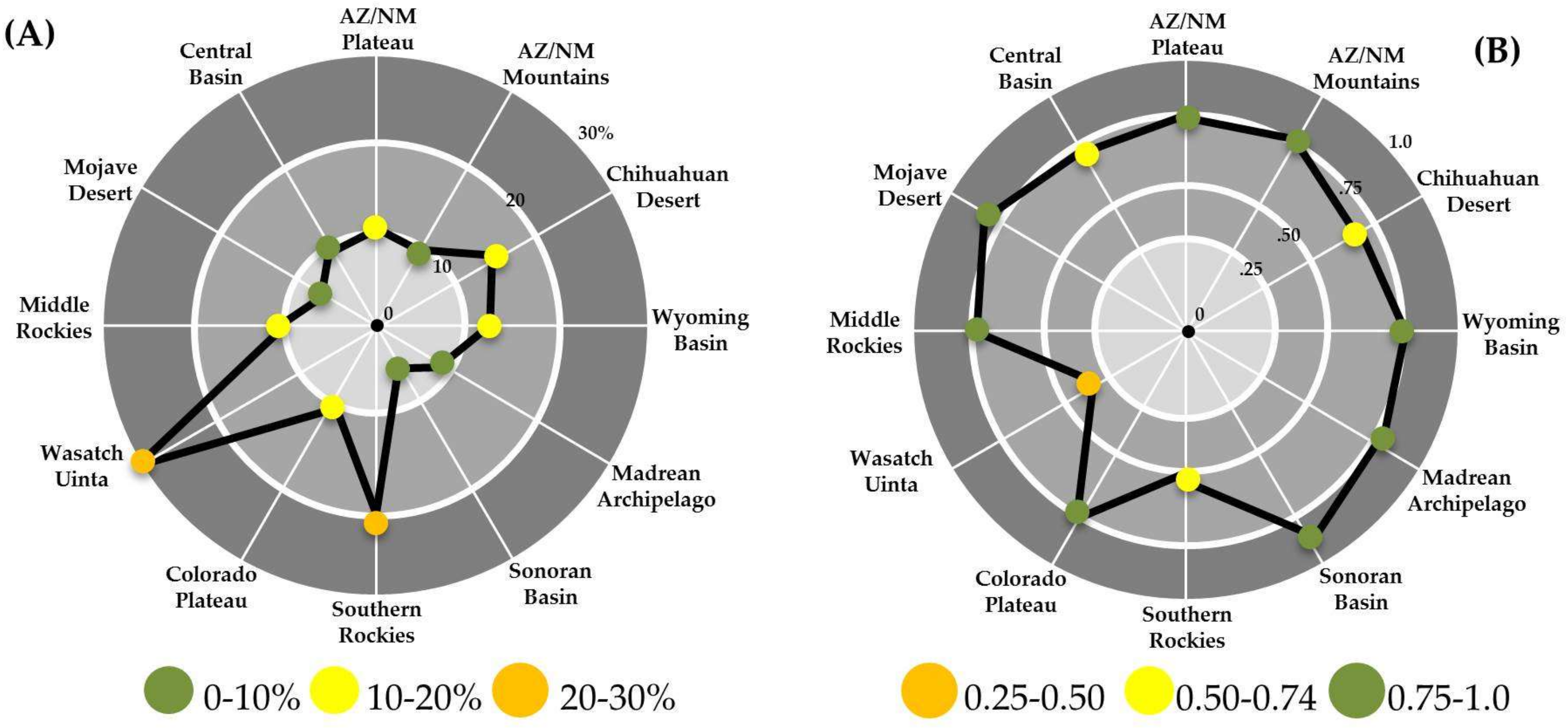
3.2. Riparian Vegetation

Each of the vegetation classification models were evaluated independently, separated by EPA Level III ecoregion. Overall, models performed reasonably well in the classification of riparian vegetation, with models in some ecoregions outperforming other ecoregions. Each final model was built using a slightly different combination of environmental predictors, which was expected based on the high degree of environmental heterogeneity between EPA ecoregions (Figure 4). Near-infrared reflectance and thermal values (band 5 and band 11 of Landsat 8), and indices including NDVI, SAVI, mNDWI, tasseled cap brightness and wetness, and topography (slope and elevation) were retained most often in our final models across ecoregions.
The random forests classification models had a median out of bag (OOB) error of 10.2% (range 4.2–28.8%), median Kappa of 0.80 (range 0.42–0.90) and class errors ranging from 5–30% (median 10%) (Figure 5). Appendix C shows out of bag and cross-validated error, confusion matrices, class errors, as well as user’s and producer’s accuracies for each individual model. Representative examples of riparian vegetation model predictions across four major ecotones are provided in Figure 6. Most models performed well. However, models located primarily in coniferous forest environments (e.g., Wasatch Uinta ecoregions) performed poorly in comparison to those carried out in arid riparian systems (e.g., Sonoran Basin; Figure 5).

3.3. Dataset Availability

Our final valley bottom extent polygons and riparian vegetation maps analysis are available freely online through the Dryad Digital Repository at https://0-doi-org.brum.beds.ac.uk/10.5061/dryad.3g55sv8. The riparian vegetation dataset is distributed in a raster format, with a value of “0” corresponding to riparian vegetation absence and a value of “100” corresponding to riparian vegetation presence for a particular pixel (Figure 6). Valley bottom extents, which we have defined as a proxy for the spatial extent of the riparian corridor, are distributed as polygons in shapefile format. Data files can be obtained for the entire Colorado River Basin or for each individual ecoregion based upon the user’s preference.

4. Discussion

We created CO-RIP, a basin-wide riparian corridor extent and riparian vegetation distribution dataset that has broad applications in riparian area management, wildlife surveys and conservation, invasive species management and ecohydrological research. The spatial distribution and resolution of this dataset will allow for researchers to conduct landscape scale analyses that would not have been possible for the Colorado River Basin in the past. Our methods integrating topographic delineation of valley bottoms combined with vegetation classification modelling allowed for a consistent definition of riparian corridors and vegetation across an extremely ecologically diverse study area. This process also emphasized the challenges associated with creating a dataset of this scale in a setting where no conclusive definition of “riparian corridors” or “riparian vegetation” exists.
The dataset produced through these analyses was created to match our definition of “riparian corridors” and “riparian vegetation”, and as such, should not be construed to fully represent any of the definitions of riparian corridors put forth in past research or in governmental reports. Instead, we integrated specific concepts from past research and governmental guidance to craft a definition (Figure 2) and corresponding dataset that was possible to accurately produce using only guided image interpretation, and topographic, GIS, and remote sensing based analyses. While our definition fit well within a remote sensing based modelling framework, modelling riparian vegetation within specific habitats presented some challenges.
We found our definition and associated analyses fit and performed well in arid regions of the Colorado River Basin where riparian vegetation was spectrally discernable from non-riparian vegetation. In these areas, the availability of water provided by riparian corridors creates a strikingly different composition of plant species and vibrancy of vegetation that is clearly interpretable and discernable using high resolution imagery to conduct sampling, coupled with Landsat spectral information (Figure 6). However, in high elevation areas with dense coniferous vegetation, particularly in the Wasatch Uinta Mountains and Southern Rockies ecoregions, the consistent presence of moist coniferous forests made it difficult to interpret differences between riparian and upland vegetation, as the vegetative gradient was largely consistent from the upland to the water feature’s bank. While we only sampled riparian vegetation presence locations where vegetation was clearly unique from the upland, models in these areas are likely underestimating riparian vegetation within the valley bottom (Figure 6). This confusion also resulted in poorer model statistics in these ecoregions. Users must employ caution, especially in these ecoregions, by ensuring that their particular application of this dataset fits the definition set forth by the authors (Figure 2), which requires riparian vegetation to be different in either observed species composition or vegetative vigor from that of the upland to be classified as such. A definition that is more inclusive in the classification of coniferous vegetation as riparian vegetation, even if it is not easily distinguishable from that of upland vegetation, may be more appropriate in these particular areas, but was outside the scope of this research. We also conducted image based sampling for riparian vegetation throughout many canyons (Figure 6). Issues presented by shadows, pixel size, canyon depth, and occlusion complicate vegetation mapping with remotely sensed imagery. While these limitations are certainly important considerations in the application of our dataset in subsequent analyses, these issues manifest in a relatively small portion of the study area overall, and we are confident the dataset is broadly applicable to a wide variety of research.
This dataset can support novel research on the potential effects of riparian habitat fragmentation, and inform future land-use and riparian network connectivity planning in the basin [57]. The riparian vegetation map could be immediately applied to prioritize potential areas for restoration and conservation activities in the Colorado River Basin [58]. For example, in the western US, there are more than 70 avian species considered to be riparian habitat obligate or dependent [59,60]. While many studies describe the importance and use of riparian habitat by such species, few have quantified habitat use or population densities at landscape scales [20,61,62] in part because of a previous lack of a spatially explicit riparian dataset. Thus, there are many potential applications of the dataset, and these ideas represent only a subset of the research made possible through the CO-RIP.
Recent advancements in access to remote sensing data and the computational power provided by cloud computing enabled this project to be successfully carried out in a relatively short period of time (~1 yr). The ability to access, process, and mosaic high resolution imagery for interpretation, as well as to process, mosaic, and composite Landsat images across a growing season in seconds would have been impossible for a standard user just years ago. We suggest that users interested in utilizing these types of geo-information across large spatial extents or implementing our riparian vegetation modelling framework to highly consider the use of cloud computing platforms [34] to expedite data processing, modelling, and image interpretation.
The Valley Bottom Extraction Tool [33] was a valuable and approachable tool for delineating valley bottoms across vast river networks. It was time-efficient and, in a qualitative sense, an accurate representation of valley bottoms and riparian corridors, especially considering the extensive region of interest. The flexibility of visually validating and manual editing of valley bottom results allows for an enhanced product that characterizes the diverse nature of valley bottoms. We do, however, recommend manual editing be conducted by scientists with an expert understanding of hydrological and ecological characteristics of the study region; erroneous manual editing could significantly degrade the V-BET algorithm results.
While the use of EPA ecoregions to subset a study area for modelling is a standard practice [63,64], we believe parsing the study site by ecoregion likely improved model performance, as these boundaries helped create a more spectrally consistent definition of riparian vegetation within specific regions of our expansive study region. While these ecoregion boundaries are not perfect delineations of separate habitat types, in broad scale analyses like those employed in this study, they can serve as a useful tool to collect largely spectrally consistent training samples. While we used composited Landsat imagery to ensure the availability of cloud free imagery in our study area, with additional time and resources a multi-temporal approach could be employed to refine these models. Including imagery that represented spring, summer, and fall seasons in each of these models (a “multi-temporal modelling framework”) [65,66] could help capture vegetation with short leaf on periods and improve classification discrimination between riparian vegetation and irrigated agriculture.
Finally, we took care to collect a sufficient number of training samples in each ecoregion to effectively capture the full range of cover that could be present within the boundaries of a Landsat pixel. However, this method could likely be improved by estimating the area of a pixel vegetated by riparian vegetation, instead of simply the presence and absence of vegetation, and then working in a regression based modelling framework instead of a presence/absence classification. This could likely improve area estimates and would make samples more representative of what is present within the boundaries of a specific pixel. While this could complicate sampling and modelling, and require additional time and resources, we believe it should be considered in future digital sampling designs created for mapping of riparian vegetation.

5. Conclusions

The research and analyses conducted to produce the “CO-RIP” datasets provides a valuable contribution to methodology to delineate riparian area and corridor extent networks at the landscape scale, and could be further applied in new areas or across larger spatial extents. Satellite image acquisition, image interpretation and modelling using newly available interfaces, advancements and availability of higher resolution topographic models, and the availability of peer-reviewed, open source valley bottom network models allow for regional scale analyses that would have been prohibitively time consuming and costly just years ago. The “riparian corridor” and “riparian vegetation” definitions adopted in this study provide a standardized, remote sensing and GIS-friendly framework for mapping of riparian areas in the future. Still, moist coniferous forest environments represent a challenging ecotype to separate riparian vegetation from upland vegetation because of the spectral consistency across these ecotones. Further research is warranted on the differentiation of upland coniferous vegetation from that present in the riparian corridor, and may require on the ground sampling to improve future landscape-scale models. Finally, this research resulted in a novel dataset for the Colorado River Basin, titled “CO-RIP” that provides ecologists, conservationists, and land managers with the highest spatial resolution delineation of riparian areas and valley bottom networks available for the ecologically diverse and topographically complex basin environment.

Author Contributions

Conceptualization, B.D.W., P.H.E., N.E.Y., A.G.V., A.M.W., R.A. and C.J.; Formal analysis, B.D.W., N.E.Y., A.G.V., A.M.W., S.L.C., R.G., E.Z.H., R.A., M.L.V., A.V., T.M. and D.C.; Funding acquisition, P.H.E.; Investigation, P.H.E; Methodology, B.D.W., P.H.E., N.E.Y., A.G.V. and A.M.W.; Project administration, P.H.E. and N.E.Y.; Resources, P.H.E.; Supervision, P.H.E.; Writing—original draft, B.D.W., P.H.E., N.E.Y., A.G.V., A.M.W., S.L.C., R.G., E.Z.H., R.A., M.L.V., A.V., T.M., D.C. and C.J.; Writing—review & editing, B.D.W., P.H.E., N.E.Y., A.G.V., A.M.W., S.L.C., R.G., E.Z.H., R.A., M.L.V., A.V., T.M., D.C. and C.J.

Funding

This research was funded by the Walton Family Foundation, grant number 2016-1805.

Acknowledgments

We would like to thank Chanin Tilakamonkul, Emily Campbell, Audrey Martinez, Julia Sullivan, and Oliver Miltenberger for assisting with sample collection. Thank you to all who contributed data, expertise, and time in the creation of this manuscript. Thank you to Tom Stohlgren for offering an initial review of the draft manuscript prior to submission. We greatly appreciate the helpful suggestions provided by four anonymous reviewers. Any use of trade, firm, or product names is for descriptive purposes only and does not imply endorsement by the US Government.

Conflicts of Interest

The authors declare no conflict of interest. The funders had no role in the design of the study; in the collection, analyses, or interpretation of data; in the writing of the manuscript, and in the decision to publish the results.

Appendix A

Description of the twelve Level III ecoregions within the extent of the study area (Modified from [30])
Ijgi 07 00397 i001aIjgi 07 00397 i001bIjgi 07 00397 i001cIjgi 07 00397 i001dIjgi 07 00397 i001e

Appendix B

Number of riparian vegetation presence and absence points collected within each ecoregion.
Ijgi 07 00397 i002

Appendix C

Detailed evaluation statistics from all riparian vegetation model runs.
Ijgi 07 00397 i003

References

  1. Poff, N.L.; Allan, J.D.; Bain, M.B.; Karr, J.R.; Prestegaard, K.L.; Richter, B.D.; Sparks, R.E.; Stromberg, J.C. The Natural Flow Regime. BioScience 1997, 47, 769–784. [Google Scholar] [CrossRef] [Green Version]
  2. Naiman, R.J.; Decamps, H.; Pollock, M. The Role of Riparian Corridors in Maintaining Regional Biodiversity. Ecol. Appl. 1993, 3, 209–212. [Google Scholar] [CrossRef] [PubMed] [Green Version]
  3. Loomis, J.; Kent, P.; Strange, L.; Fausch, K.; Covich, A. Measuring the total economic value of restoring ecosystem services in an impaired river basin: results from a contingent valuation survey. Ecol. Econ. 2000, 33, 103–117. [Google Scholar] [CrossRef]
  4. Salo, J.A.; Theobald, D.M. A Multi-scale, Hierarchical Model to Map Riparian Zones. River Res. Appl. 2016, 32, 1709–1720. [Google Scholar] [CrossRef]
  5. Johnson, A.S. The Thin Green Line: Riparian Corridors and Endangered Species in Arizona and New Mexico. In Defense of Wildlife: Preserving Communities and Corridors; Mackintosh, E.S., Fitzgerald, J., Kloepfer, D., Eds.; Defenders of Wildlife: Washington, DC, USA, 1989; pp. 35–46. [Google Scholar]
  6. Swift, B.L. Status of Riparian Ecosystems in the United States. J. Am. Water Resour. Assoc. 1984, 20, 223–228. [Google Scholar] [CrossRef]
  7. Dahl, T.E. Wetlands Losses in the United States 1780’s to 1980’s; US Department International Fish Wildlife Service: Washington, DC, USA, 1990; p. 21.
  8. Richardson, D.M.; Holmes, P.M.; Esler, K.J.; Galatowitsch, S.M.; Stromberg, J.C.; Kirkman, S.P.; Pyšek, P.; Hobbs, R.J. Riparian vegetation: Degradation, alien plant invasions, and restoration prospects. Divers. Distrib. 2007, 13, 126–139. [Google Scholar] [CrossRef]
  9. Poff, B.; Koestner, K.A.; Neary, D.G.; Henderson, V. Threats to Riparian Ecosystems in Western North America: An Analysis of Existing Literature. J. Am. Water Resour. Assoc. 2011, 47, 1241–1254. [Google Scholar] [CrossRef]
  10. Violin, C.R.; Cada, P.; Sudduth, E.B.; Hassett, B.A.; Penrose, D.L.; Bernhardt, E.S. Effects of urbanization and urban stream restoration on the physical and biological structure of stream ecosystems. Ecol. Appl. Publ. Ecol. Soc. Am. 2011, 21, 1932–1949. [Google Scholar] [CrossRef]
  11. Kauffman, J.B.; Krueger, W.C. Livestock impacts on riparian ecosystems and streamside management implications—A review. Rangel. Ecol. Manag. J. Range Manag. Arch. 1984, 37, 430–438. [Google Scholar] [CrossRef]
  12. Bunn, S.E.; Arthington, A.H. Basic principles and ecological consequences of altered flow regimes for aquatic biodiversity. Environ. Manag. 2002, 30, 492–507. [Google Scholar] [CrossRef]
  13. Multi-Resoultion Land Characteristics Consortium (MRLC). Available online: https://www.mrlc.gov/nlcdshrub.php (accessed on 18 May 2018).
  14. Homer, C.; Dewitz, J.; Yang, L.; Jin, S.; Danielson, P.; Xian, G.; Coulston, J.; Herold, N.; Wickham, J.; Megown, K. Completion of the 2011 National Land Cover Database for the Conterminous United States—Representing a Decade of Land Cover Change Information. Photogramm. Eng. Remote Sens. 2015, 81, 346–354. [Google Scholar] [CrossRef]
  15. LANDFIRE. Available online: https://www.landfire.gov/evt.php (accessed on 18 May 2018).
  16. Lowry, J.; Ramsey, R.D.; Thomas, K.; Schrupp, D.; Sajwaj, T.; Kirby, J.; Waller, E.; Schrader, S.; Falzarano, S.; Langs, L.; et al. Mapping moderate-scale land-cover over very large geographic areas within a collaborative framework: A case study of the Southwest Regional Gap Analysis Project (SWReGAP). Remote Sens. Environ. 2007, 108, 59–73. [Google Scholar] [CrossRef]
  17. Copernicus Land Monitoring Service. Available online: https://land.copernicus.eu/local/riparian-zones (accessed on 15 August 2018).
  18. National Park Service (NPS). Final Environmental Impact Statement, Colorado River Management Plan; US Department of the Interior: Grand Canyon National Park, AZ, USA, 2005; pp. 151–157.
  19. The Nature Conservancy. Available online: https://www.nature.org/?intc=nature.tnav.logo (accessed on 5 May 2018).
  20. Lower Colorado River Multi-Species Conservation Program. Final Implementation Report, Fiscal Year 2019 Work Plan and Budget, Fiscal Year 2017 Accomplishment Report; US Department of the Interior: Boulder City, NV, USA, 2018.
  21. Gregory, S.V.; Swanson, F.J.; McKee, W.A.; Cummins, K.W. An Ecosystem Perspective of Riparian Zones. BioScience 1991, 41, 540–551. [Google Scholar] [CrossRef]
  22. Knopf, F.L.; Johnson, R.R.; Rich, T.; Samson, F.B.; Szaro, R.C. Conservation of Riparian Ecosystems in the United States. Wilson Bull. 1988, 100, 23. [Google Scholar]
  23. Swanson, F.J.; Kratz, T.K.; Caine, N.; Woodmansee, R.G. Landform Effects on Ecosystem Patterns and Processes: Geomorphic features of the earth’s surface regulate the distribution of organisms and processes. BioScience 1988, 38, 92–98. [Google Scholar] [CrossRef]
  24. Congalton, R.; Birch, K.; Jones, R.; Schriever, J. Evaluating Remotely Sensed Techniques for Mapping Riparian Vegetation. Comput. Electron. Agric. 2002, 37, 113–126. [Google Scholar] [CrossRef]
  25. Goetz, S.J. Remote Sensing of Riparian Buffers: Past Progress and Future Prospects. J. Am. Water Resour. Assoc. 2006, 42, 133–143. [Google Scholar] [CrossRef]
  26. Hollenhorst, T.P.; Host, G.E.; Johnson, L.B. Scaling issues in mapping riparian zones with remote sensing data: quantifying errors and sources of uncertainty. In Scaling and Uncertainty Analysis in Ecology; Wu, J., Jones, K.B., Li, H., Loucks, O.L., Eds.; Springer: Dordrecht, The Netherlands, 2006; pp. 275–295. ISBN 978-1-4020-4662-9. [Google Scholar]
  27. Clerici, N.; Weissteiner, C.; Luisa Paracchini, M.; Boschetti, L.; Baraldi, A.; Strobl, P. Pan-European distribution modelling of stream riparian zones based on multi-source Earth Observation data. Ecol. Indic. 2013, 24, 211–223. [Google Scholar] [CrossRef]
  28. Alaibakhsh, M.; Emelyanova, I.; Barron, O.; Sims, N.; Khiadani, M.; Mohyeddin, A. Delineation of riparian vegetation from Landsat multi-temporal imagery using PCA. Hydrol. Process. 2017, 31, 800–810. [Google Scholar] [CrossRef]
  29. Kammerer, J.C. Largest Rivers in the United States (Water Fact Sheet); US Geological Survey: Reston, VA, USA, 1990; pp. 87–242. [Google Scholar]
  30. Wilken, E.; Jiménez Nava, F.; Griffith, G. North American Terrestrial Ecoregions—Level III. Commun. Environ. Coop. 2011. [Google Scholar]
  31. Macfarlane, W.W.; Gilbert, J.T.; Jensen, M.L.; Gilbert, J.D.; Hough-Snee, N.; McHugh, P.A.; Wheaton, J.M.; Bennett, S.N. Riparian vegetation as an indicator of riparian condition: Detecting departures from historic condition across the North American West. J. Environ. Manag. 2017, 202, 447–460. [Google Scholar] [CrossRef] [PubMed]
  32. Ilhardt, B.L.; Verry, E.S.; Palik, B.J. Defining riparian areas. In Riparian Management in Forests of the Continental Eastern United States; Verry, E.S., Hornbeck, J.W., Dolloff, C.A., Eds.; Lewis Publishers: New York, NY, USA, 2000; ISBN 978-1-56670-501-1. [Google Scholar]
  33. Gilbert, J.T.; Macfarlane, W.W.; Wheaton, J.M. The Valley Bottom Extraction Tool (V-BET): A GIS tool for delineating valley bottoms across entire drainage networks. Comput. Geosci. 2016, 97, 1–14. [Google Scholar] [CrossRef]
  34. Environmental Systems Research Institute (ESRI). ArcGIS 10.3.; Environmental Systems Research Institute (ESRI): Redlands, CA, USA, 2004. [Google Scholar]
  35. US Geological Survey—National Hydrography Dataset (2016). Available online: https://nhd.usgs.gov/ (accessed on 12 September 2017).
  36. Gesch, D.B.; Oimoen, M.J.; Greenlee, S.K.; Nelson, C.A.; Steuck, M.J.; Tyler, D.J. The national elevation data set. Photogramm. Eng. Remote Sens. 2002, 68, 5–32. [Google Scholar]
  37. Simley, J.D.; Carswell, W.J., Jr. The National Map-Hydrography; US Geological Survey Fact Sheet 2009-3054; US Department of the Interior: Washington, DC, USA, 2009; pp. 1–4.
  38. Seaber, P.R.; Kapinos, F.P.; Knapp, G.L. Hydrologic Unit Maps; Water Supply Paper 2294; US Geological Survey: Denver, CO, USA, 1987; p. 63. [Google Scholar]
  39. Omernik, J.M.; Griffith, G.E. Ecoregions of the Conterminous United States: Evolution of a Hierarchical Spatial Framework. Environ. Manag. 2014, 54, 1249–1266. [Google Scholar] [CrossRef] [PubMed]
  40. Edwards, T.C.; Cutler, D.R.; Zimmermann, N.E.; Geiser, L.; Moisen, G.G. Effects of sample survey design on the accuracy of classification tree models in species distribution models. Ecol. Model. 2006, 199, 132–141. [Google Scholar] [CrossRef]
  41. Elmore, W.; Beschta, R.L. Riparian areas: Perceptions in management. Rangel. Arch. 1987, 9, 260–265. [Google Scholar]
  42. Jones, G. Workplan for a Uniform Statewide Riparian Vegetation Classification; Wyoming Natural Diversity Database: Laramie, WY, USA, 1990. [Google Scholar]
  43. Crist, E.P.; Kauth, R.J. The Tasseled Cap De-Mystified. Photogramm. Eng. 1986, 52, 81–86. [Google Scholar]
  44. Baig, M.H.A.; Zhang, L.; Shuai, T.; Tong, Q. Derivation of a tasselled cap transformation based on Landsat 8 at-satellite reflectance. Remote Sens. Lett. 2014, 5, 423–431. [Google Scholar] [CrossRef]
  45. Rouse, W.; Haas, R.H. Monitoring Vegetation Systems in the Great Plains with ERTS. 9; NASA: Washington, DC, USA.
  46. Huete, A. A soil-adjusted vegetation index (SAVI). Remote Sens. Environ. 1988, 25, 295–309. [Google Scholar] [CrossRef]
  47. Xu, H. Modification of normalised difference water index (NDWI) to enhance open water features in remotely sensed imagery. Int. J. Remote Sens. 2006, 27, 3025–3033. [Google Scholar] [CrossRef]
  48. Breiman, L. Random Forests. Mach. Learn. 2001, 45, 5–32. [Google Scholar] [CrossRef] [Green Version]
  49. Liaw, A.; Wiener, M. Classification and Regression by RandomForest. R News 2002, 2, 18–22. [Google Scholar]
  50. Gislason, P.O.; Benediktsson, J.A.; Sveinsson, J.R. Random Forests for Land Cover Classification. Pattern Recognit. Lett. 2006, 27, 294–300. [Google Scholar] [CrossRef]
  51. Evans, J.S.; Murphy, M.A. rfUtilities: Random Forests Model Selection and Performance Evaluation. R package version 1.0-2. 2015. Available online: http://cran.r-project.org/pack-age = rfUtilities (accessed on 6 January 2017.
  52. R Development Core Team. R: A Language and Environment for Statistical Computing; The R Foundation for Statistical Computing; R Development Core Team: Vienna, Austria; ISBN 3-900051-07-0.
  53. Murphy, M.A.; Evans, J.S.; Storfer, A. Quantifying Bufo boreas connectivity in Yellowstone National Park with landscape genetics. Ecology 2010, 91, 252–261. [Google Scholar] [CrossRef] [PubMed]
  54. Sullivan, P.F.; Mulvey, R.L.; Brownlee, A.H.; Barrett, T.M.; Pattison, R.R. Warm summer nights and the growth decline of shore pine in Southeast Alaska. Environ. Res. Lett. 2015, 10, 124007. [Google Scholar] [CrossRef] [Green Version]
  55. Strobl, C.; Boulesteix, A.-L.; Kneib, T.; Augustin, T.; Zeileis, A. Conditional variable importance for random forests. BMC Bioinform. 2008, 9, 307. [Google Scholar] [CrossRef] [PubMed] [Green Version]
  56. Kohavi, R. A Study of Cross-Validation and Bootstrap for Accuracy Estimation and Model Selection; Morgan Kaufmann Publishers Inc.: San Francisco, CA, USA, 1995; pp. 1137–1143. [Google Scholar]
  57. Fremier, A.K.; Kiparsky, M.; Gmur, S.; Aycrigg, J.; Craig, R.K.; Svancara, L.K.; Goble, D.D.; Cosens, B.; Davis, F.W.; Scott, J.M. A riparian conservation network for ecological resilience. Biol. Conserv. 2015, 191, 29–37. [Google Scholar] [CrossRef] [Green Version]
  58. Macfarlane, W.W.; McGinty, C.M.; Laub, B.G.; Gifford, S.J. High-resolution riparian vegetation mapping to prioritize conservation and restoration in an impaired desert river. Restor. Ecol. 2016, 25, 333–341. [Google Scholar] [CrossRef]
  59. Brown, B.T.; Trosset, M.W. Nesting-Habitat Relationships of Riparian Birds along the Colorado River in Grand Canyon, Arizona. Southwest. Nat. 1989, 34, 260–270. [Google Scholar] [CrossRef]
  60. Rich, T.D. Using Breeding Land Birds in the Assessment of Western Riparian Systems. Wildl. Soc. Bull. 2002, 30, 1128–1139. [Google Scholar]
  61. Brand, L.A.; White, G.C.; Noon, B.R. Factors Influencing Species Richness and Community Composition of Breeding Birds in a Desert Riparian Corridor. Condor 2008, 110, 199–210. [Google Scholar] [CrossRef]
  62. Trathnigg, H.K.; Phillips, F.O. Importance of Native Understory for Bird and Butterfly Communities in a Riparian and Marsh Restoration Project on the Lower Colorado River, Arizona. Ecol. Restor. 2015, 33, 395–407. [Google Scholar] [CrossRef]
  63. Coops, N.C.; Ferster, C.J.; Waring, R.H.; Nightingale, J. Comparison of three models for predicting gross primary production across and within forested ecoregions in the contiguous United States. Remote Sens. Environ. 2009, 113, 680–690. [Google Scholar] [CrossRef] [Green Version]
  64. Liu, J.; Vogelmann, J.; Zhu, Z.; Key, C.; Sleeter, B.; Price, D.; Chen, J.; Cochrane, A.M.; Eidenshink, J.M.; Howard, S.; et al. Estimating California ecosystem carbon change using process model and land cover disturbance data: 1951–2000. Ecol. Model. 2011, 222, 2333–2341. [Google Scholar] [CrossRef]
  65. Evangelista, P.H.; Stohlgren, T.J.; Morisette, J.T.; Kumar, S. Mapping Invasive Tamarisk (Tamarix): A Comparison of Single-Scene and Time-Series Analyses of Remotely Sensed Data. Remote Sens. 2009, 1, 519–533. [Google Scholar] [CrossRef] [Green Version]
  66. West, A.M.; Evangelista, P.H.; Jarnevich, C.S.; Kumar, S.; Swallow, A.; Luizza, M.W.; Chignell, S.M. Using multi-date satellite imagery to monitor invasive grass species distribution in post-wildfire landscapes: An iterative, adaptable approach that employs open-source data and software. Int. J. Appl. Earth Obs. Geoinf. 2017, 59, 135–146. [Google Scholar] [CrossRef]
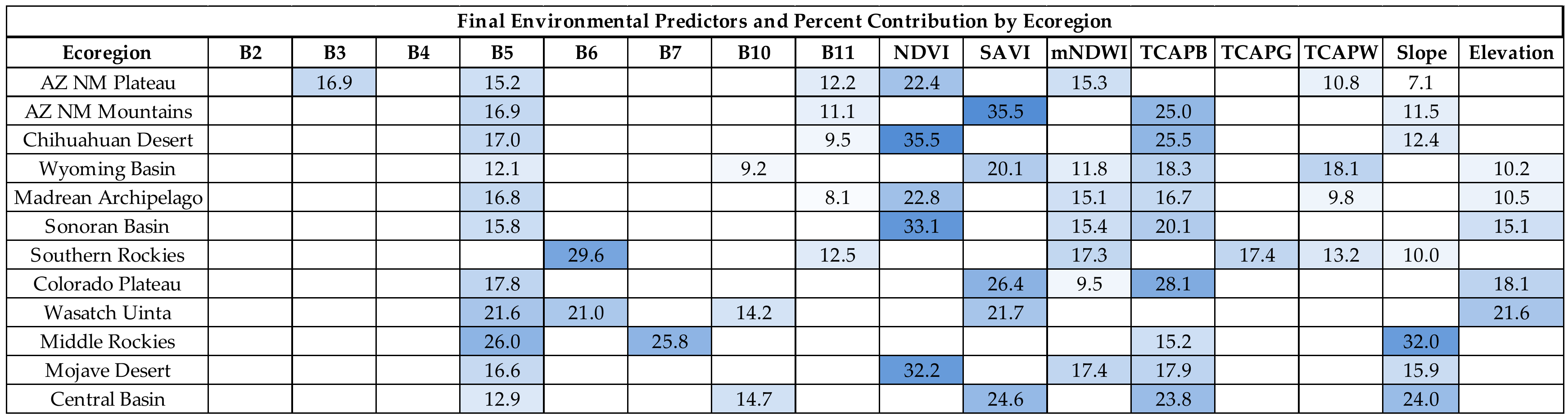
Figure 1. The study area extent, which encompasses the entire US portion of the Colorado River Basin, classified by EPA Level 3 ecoregion.
Ijgi 07 00397 g001
Figure 2. An overview of the process used to delineate riparian vegetation. First, a decision tree process was used by trained image interpreters to evaluate whether a sampled location should be classified as “riparian vegetation presence” or “riparian vegetation absence”. These training points were then used to build classification models of riparian vegetation presence and riparian vegetation absence, and applied as a prediction across each ecoregion. In post-processing, vegetation classified as riparian vegetation that was outside of the valley bottom was then excluded using the valley bottom extraction tool (V-BET) GIS output.
Ijgi 07 00397 g002
Figure 3. Example subsets of valley bottom extent results across three different environments. Green lines represent the external boundaries of the valley bottom, which we define as the riparian corridor. Vegetation outside of valley bottoms is considered to be outside of the riparian corridor. Within the valley bottom, riparian vegetation was separated from non-riparian vegetation such as agriculture (example in middle image) using riparian vegetation classification.
Ijgi 07 00397 g003
Figure 4. Final predictors included in each random forests classification model. Each row represents a separate model for the specified ecoregion. The numbers in each row are the relative percent contribution of each predictor in each individual model. White boxes with numbers represent the lowest relative contribution, light blue a medium relative contribution, and darker blue a high relative contribution. White boxes with no numbers correspond to predictors that were not retained in the final models, and therefore did not contribute to the final model. From Landsat 8; B2: Blue band; B3: Green band; B4: Red band; B5: Near infrared band; B6: Shortwave infrared 1 band; B7: Shortwave infrared 2 band; B10: Thermal infrared 1 band; B11: Thermal infrared 2 band; NDVI: Normalized Difference Vegetation Index; SAVI: Soil Adjusted Vegetation Index; mNDWI: Modified Normalized Difference Water Index; TCAP B, G, W: Tasseled cap brightness, greenness, and wetness.
Ijgi 07 00397 g004
Figure 5. Radar charts displaying cross-validated error rates (A) (0–100%) and Kappa (B) (0–1) for each of the final random forests classification models. Model performance is best when error rates (A) are closer to the center and when kappa values (B) are closer to the perimeter of the chart.
Ijgi 07 00397 g005
Figure 6. Representative examples of our final results in four different ecoregions. (A) Displays the differentiation of agriculture from riparian vegetation and the delineation of the riparian corridor; (B) displays delineation of riparian vegetation in narrow, sinuous canyon environments, which can be challenging using remotely sensed datasets; (C) displays an underprediction of riparian vegetation that is characteristic of results seen in moist coniferous forest environments; (D) displays the delineation of riparian vegetation in arid environments, where models performed extremely well in delineating riparian vegetation from non-riparian vegetation and landscape characteristics.
Ijgi 07 00397 g006
Table 1. The environmental predictors that were employed in each random forests classification model. Predictors were subsequently pared down through variable selection.
Environmental PredictorsApplication
Landsat Spectral Reflectance and Thermal Measurements *Used to capture spectral variability available from Landsat TM/OLI sensors
Normalized Difference Vegetation Index (NDVI)Indicator of live green vegetation
Soil Adjusted Vegetation Index (SAVI)An adjusted live vegetation index that accounts for soil brightness
Modified Normalized Difference Water Index (mNDWI)An indicator of water presence that reduces the influence of spectral mixing caused by vegetation and urban environments
Tasseled Cap Transformation (Brightness, Greenness, Wetness)Linear combinations of original reflectance bands that results in interpretable ecological characteristics
Topography (Slope, Elevation)Used to capture potential topographic patterns of riparian vegetation
* The following bands from Landsat 8 OLI/TIRS were applied: Red, green, blue, near infrared, shortwave infrared and thermal bands. The panchromatic, cirrus, and coastal/aerosol bands were excluded from all random forests classification models.

