Article

From Global Goals to Local Gains—A Framework for Crop Water Productivity

by
Megan Leigh Blatchford
1,*,
Poolad Karimi
2,
W.G.M. Bastiaanssen
3,4 and
Hamideh Nouri
5,6
1
Department of Water Resources, Faculty of Geo-Information Science and Earth Observation (ITC), University of Twente, Enschede 7500 AE, The Netherlands
2
Water Science and Engineering Department, IHE Delft Institute for Water Education, Delft 2611 AX, The Netherlands
3
Integrated Water Systems and Governance Department, IHE Delft Institute for Water Education, Delft 2611 AX, The Netherlands
4
Department of Water Resources Management, Faculty of Civil Engineering and Geosciences, Delft University of Technology, Delft 2600 GA, The Netherlands
5
Department of Water Engineering and Management, Faculty of Engineering Technology, University of Twente, Enschede 7500 AE, The Netherlands
6
Division of Agronomy, University of Göttingen, Göttingen 37075, Germany
*
Author to whom correspondence should be addressed.
ISPRS Int. J. Geo-Inf. 2018, 7(11), 414; https://0-doi-org.brum.beds.ac.uk/10.3390/ijgi7110414
Submission received: 20 September 2018 / Revised: 22 October 2018 / Accepted: 23 October 2018 / Published: 25 October 2018
(This article belongs to the Special Issue Geo-Information and the Sustainable Development Goals (SDGs))

Abstract

:
Crop water productivity (CWP) has become a recognised indicator in assessing the state of Sustainable Development Goals (SDG) 6.4—to substantially increase water use efficiency. This indicator, while useful at a global scale, is not comprehensive at a local scale. To fill this gap, this research proposes a CWP framework, that takes advantage of the spatio-temporal availability of remote sensing, that identifies CWP goals and sub-indicators specific to the needs of the targeted domain. Three sub-indicators are considered; (i) a global water productivity score (GWPS), (ii) a local water productivity score (LWPS) and (iii) a land and water use productivity score (YWPS). The GWPS places local CWP in the global context and focuses on maximised CWP. The LWPS differentiates yield zones, normalising for potential product, and focuses on minimising water consumption. The YWPS focuses simultaneously on improving land and water productivity equally. The CWP framework was applied to potato in the West Bank, Palestine. Three management practices were compared under each sub-indicator. The case study showed that fields with high and low performance were different under each sub-indicator. The performance associated with different management practices was also different under each sub-indicator. For example, a winter rotation had a higher performance under the YWPS, the fall rotation had a higher performance under the LWPS and under the GWPS there was little difference. The results showed, that depending on the basin goal, not only do the sub-indicators required change, but also the management practices or approach required to reach those basin goals. This highlights the importance of providing a CWP framework with multiple sub-indicators, suitable to basin needs, to ensure that meeting the SDG 6.4 goal does not jeopardise local objectives.

Graphical Abstract

1. Introduction

There is mounting pressure for the agricultural sector to increase crop production between 60 and 110% by 2050 [1], in order to ensure future food security based on the demands of a growing population. However, while there is increasing demand of agricultural output, agriculture at a global scale is facing multiple limitations on inputs, in particular, water and land. The consumption of land and water resources are occurring at a faster rate than the global regeneration [2,3,4,5,6].
Crop water productivity (CWP) [kg m−3], an indicator for water use efficiency (WUE), aims to integrate land productivity in conjunction with water productivity. Since food security remains the primary goal of the agricultural sector, measures to limit water consumption in agriculture must not come at the cost of curbing food production. Hence, improving CWP, and subsequently WUE, is gaining attention in addressing the issue of increasing food demand with increasing water limitations [7,8]. This has been recognised by the United Nations (UN) Sustainable Development Goals (SDGs) which stipulate that agricultural productivity should be doubled by 2030 (SGD2.3) and that WUE must be substantially increased (SDG6.4) [9]. The UN Food and Agricultural Organisation (FAO) and International Water Management Institute (IWMI) have already initiated programs aimed at measuring and monitoring CWP—Water Productivity Open-access Portal (WaPOR) (https://wapor.apps.fao.org/home/1).
CWP evolved from the terms WUE and water productivity (WP). Water use requirements of plants were first studied in the early 1900s by weighing containers [10]. This was then constrained to the ratio of plant production to evapotranspiration for a unit area [11]. In the 1950s and 1960s this was scaled to field and termed WUE [12,13,14]. Tanner and Sinclair [15], summarised the literature and defined WUE as the biomass of water accumulated per unit of water transpired (T) and evaporated (E) per unit crop area. Modern WUE is commonly used by irrigation engineers to assess the efficiency of water delivery or supply, whereas WP distinctly refers to the water consumed through actual evapotranspiration (ETa). This WP term was further expanded to consider beneficial outputs, e.g., physical yield or economic, rather than purely the plant production [16]. Finally, CWP, was developed to specifically define the physical crop production in terms of fresh yield to the ETa:
CWP   ( kg   m 3 ) = Yield   ( kg   ha 1 ) ETa   ( mm   season 1 ) × 10
This definition considers only actual ETa which accounts for water that is consumed, and therefore no longer available to other uses. ETa consists of soil evaporation (E) and plant transpiration (T).
Yield and transpiration has been shown to have a fixed positive linear relationship [17], while the relationship between the yield and the evapotranspiration has substantial variability. This variability stems from differences that include: environmental factors—such as climate conditions [18,19], soil type [20,21,22], and soil salinity [16,23,24]; crop factors such as—harvest index and cultivar type [24]; and management practices such as—irrigation [17,25,26], nutrient availability [27], soil management [28] and pest and disease management [23]. Thus, causes of low CWP and ways to improve it may differ from one case to another. These improvements aim at closing the gap between the current state of the CWP and the upper limit that is defined by the linear relationship between yield and ETa.
While there is consensus that CWP improvement will help in meeting growing food demands under resource constraints, devising action oriented strategies is required to help translate the theoretical scope for improvement to real on the ground gains. To be effective, such strategies must be case specific and be informed by the ground realities and needs, rather than being generalised solutions that are expected to work everywhere. The first step in this direction is to set CWP goals that consider local potentials, opportunities and limitations. Most CWP studies have developed either statistics [29,30] or maps [31,32] on a global scale, or identified that there is scope for global scale CWP improvement [33].
Benchmarking of CWP can be assessed at global or local scales. At the global scale, although interesting, it is difficult to compare CWP performance considering the climatic differences that limit crop growth. For instance, the first benchmarking was undertaken at a global scale, where values of CWP, segregated by crop, were compiled and the benchmark was set as the 95% percentile [34] in one instance, and a 90% percentile in another [35]. CWP benchmark maps were made for wheat as the average values for future evaluations and performance comparisons [36]. On a local scale, few basins have been studied, in terms of a CWP goals. The CWP of the Nile Basin was mapped to understand the variation across the basin and analyse the way to improve it under different cropping systems [37,38]. The CWP in the Indus Basin was estimated and the CWP of users against their yield were plotted on a scatter plot [39,40]. A distinct cluster of fields with a much higher CWP, distinguished as the ‘bright spot’, were identified as the goal. Areas with lowest CWP were distinguished as ‘hot spots’ and were considered to be the areas where most improvements could be made.
Most recently a global water productivity score (GWPS) and a water productivity score determined by crop yield zone (WPS) was developed [41]. The GWPS method utilises a standard scale to score the CWP against global CWP values after climatic normalisation, to account for varying climates across the globe. The WPS sub-divides the CWP into yield zones. The same standard scale is used for the score within each yield zone. This essentially defines the upper boundary function of the CWP plotted against the yield as the goal. The upper boundary being the function that defines the upper percentile (e.g., 99th percentile) CWP of a given yield.
Remote sensing is becoming the most prolific method to estimate and evaluate CWP. Remote sensing offers the spatial resolution and extent to assess CWP from farm to continental scale. Each study in the previous paragraph used remote sensing in defining the spatiotemporal variation in CWP and in assigning CWP scores. WaPOR provides open access to satellite-based ETa and biomass datasets, specifically for the purpose of estimating CWP from local to global scales. Open access satellite imagery now provides near real-time data at varying spatial and temporal resolutions from: 10 m with 10-day return period (Sentinel 2), 30 m with 16-day return period (Landsat), 100 m with daily return period (Proba-v), and 250 m with a 1 to 2-day return period (MODIS, Sentinel 3).
A CWP framework can not only help to monitor CWP, but evaluate CWP performance based on relevant goals. It is necessary to consider a CWP framework in order to progress from monitoring ‘where are we’ to evaluate: (i) ‘where are we going’, (ii) ‘what are we trying to achieve’, (iii) ‘how much improvement is needed’ and (iv) ‘how will we get there’. A CWP framework can aid in standardising an approach for setting CWP targets, by connecting appropriate sub-indicators (i.e., where are we going) relevant to basin goals (i.e., what are we trying to achieve). Sub-indicators can then help answer ‘how much improvement is needed’ and ‘how will we get there’ by specifying not only the local target but the approach.
The paper will first identify sub-indicators to CWP. The local target associated within the sub-indicators are also defined. Then, a CWP framework is developed to link the sub-indicators to basin needs. The CWP framework is then applied to a case study, potatoes in the West Bank, Palestine. The CWP is estimated, taken as the current situation, and the scores derived, using remote sensing techniques. The suitability and limitations of using each CWP sub-indicator, in the context of the framework, for the case study is then discussed.

2. Materials and Methods

The methodology will first define the CWP scoring methods, or sub-indicators. Secondly, the CWP framework will be described, which will consider each when each CWP scoring method should be applied. Finally, the case study area where the CWP framework is applied will be described, The West Bank, Palestine, along with the methodology to estimate CWP.

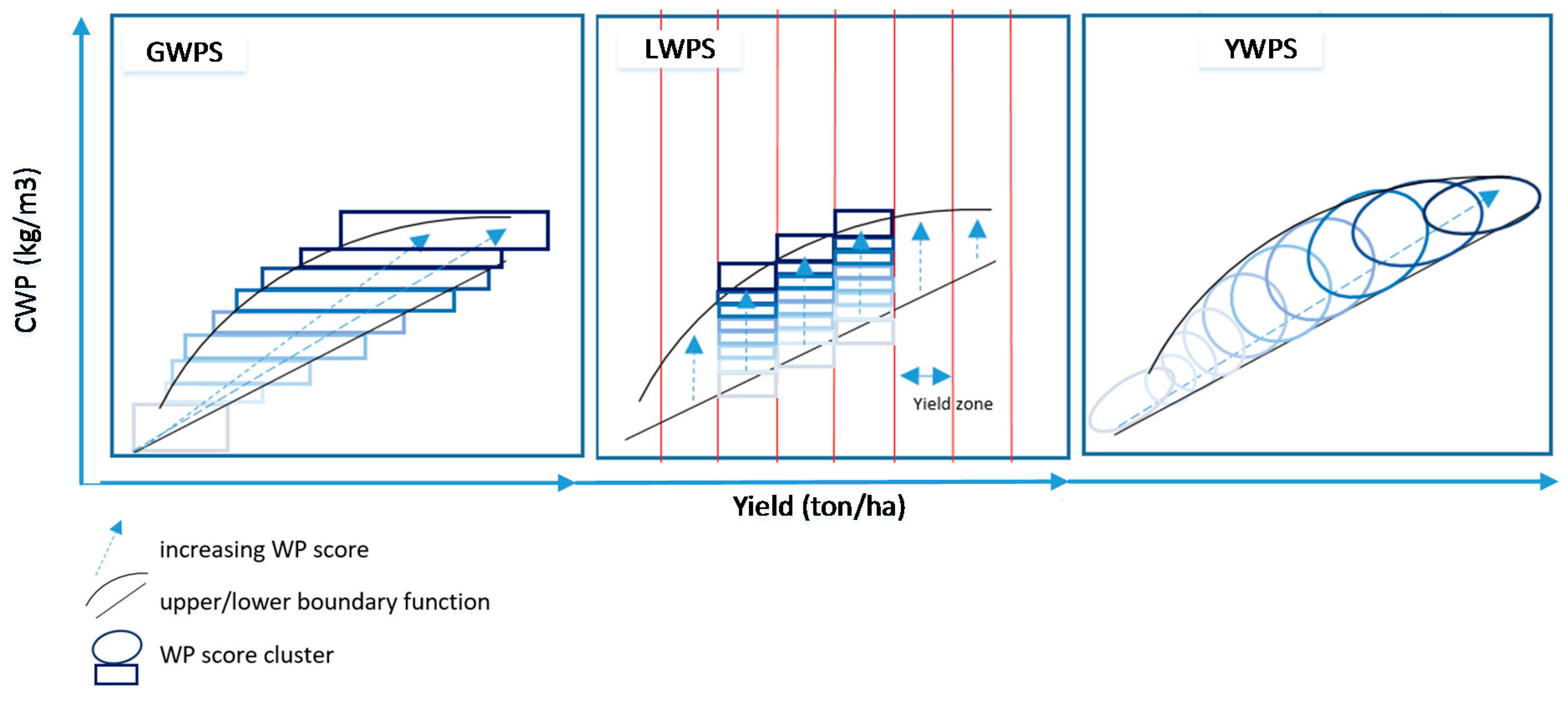
2.1. Defining Crop Water Productivity Sub-Indicators

This research includes three CWP sub-indicators which aim to take into account the different ways to improve CWP; (i) the global water productivity score (GWPS), (ii) local water productivity score (LWPS) and (iii) the land and water productivity score (YWPS). The first two methods (i and ii) were developed in previous research [41], while the third (iii) was developed in this research as a way to optimise both land and water productivity. Each scoring method identifies a different target and a different approach in reaching said target. This is intended as the basis of the CWP framework, so that the user has multiple options in trying to achieve the SDG 6.4 that is not contradictory to the basin needs.
The underlying concept of each method to determine the CWP score is shown in Figure 1, and their respective definitions and methods are described in detail throughout this chapter. The scoring methods are presented in the form of the CWP, on the y-axis, plotted against the yield, on the x-axis. The sub-indicator target is identified as the darkest rectangle or circle on each plot. Increasing scores, shown as clusters, are indicated by rectangles and circles with increasing in darkness reflecting an increasing CWP score. The clusters represent percentiles, based on scaling. The direction required to reach the target is indicated by the arrow. The black lines represent the theoretical upper and lower boundary of a given crop. The upper boundary representing the theoretical maximum CWP for a given yield and the lower boundary function representing the theoretical minimum CWP for a given yield. These boundary functions are represented this way to reflect findings that incremental gains in CWP become smaller as yield becomes higher [42]. Therefore, the upper boundary function represented as curve-linear and the lower boundary function is represented as linear. Similar upper and lower boundary function trends have been proposed in an example for rice [39,40] and the upper boundary function has been proposed in an example for maize [43].
Figure 1 shows that the GWPS target is the highest CWP, or ‘bright spot’, irrespective of yield, and that the relationship between the CWP score and the actual CWP is linear. The LWPS CWP target is set as the upper boundary function, or the upper percentile for a given yield zone, and therefore the CWP target increases with a given yield. The YWPS shows that the CWP target is achieved when both the yield the highest for a given ETa, which is also considered a bright spot.

2.1.1. Global Water Productivity Score (GWPS)

The first CWP sub-indicator, the GWPS, is aimed at maximising CWP [41]. The GWPS scores the climatically normalised CWP (CWPc) between 1 and 10, with 1 being low performing and 10 being high performing. The scores are determined by standard scaling of the recorded CWPc between the 5th percentile global CWPc and the 99th percentile global CWPc. This method sets a global CWPc as the target, which assumes that for every crop a global target can be achieved in all locations (after correction for the climatic condition of that specific location). The GWPS increases linearly with increasing normalised CWPc. Therefore, a single normalised CWPc value correlates directly to a GWPS. This approach essentially identifies ‘bright spots’ and ‘hot spots’, ‘bright spots’ being the highest performing CWPc allocated with the highest score and ‘hot spots having the lowest CWPc allocated with the lowest score.
This paper considers the GWPS on a both local and global scale, as there are many crops where global values are not available. In summary the GWPS is defined as:
GWPS—‘Maximise CWP’: Considering an upper percentile as the CWP target, adjusted for climatic variation [44], based on and adapted for local benchmarks, where [41]:
GWPS = 9 × CWPc CWPc 5 CWPc 99 CWPc 5 + 1   ( )
w h e r e   i f   C W P c > C W P c 99 ,   G W P S = 10 .
The CWPc5 and the CWPc99 are the 5th and 99th percentile CWPc refer to the 5th and 99th percentile global values for a given crop when applying the GWPS at a global scale and the 5th and 99th percentiles are the local values when applying the GWPS on a local scale. In this study, the global values have been taken from available literature on potato for this case study to obtain the 5th and 99th percentile global values. In total 29 field studies, covering 322 observations, were collected (Appendix A). The CWPc was estimated using [41]:
  CWP c = Y ET ET 0 ( a ) ET 0 ( c )
ET0(a) is the ET0 for the location and ET0(c) is the climatic average ET0, in mm season−1, worldwide, excluding the artic zone. ET0(c) was taken as the 40 year average from IWMI Climate Atlas [45]. The ET0 in SEBAL is estimated using the standard FAO 56 methodology [46]. The values for the ET0(a) used to normalise CWP to global literature on potato, if not available, were taken as the 40–year average ET0 for that location. CWP outliers are excluded by only including the 5th to 99th percentiles in the GWPS.

2.1.2. Local Water Productivity Score (LWPS)

The LWPS sub-indicator identifies a CWP target per a given yield zones. This is designed to set the upper boundary function (Figure 1) of the CWP plotted against the yield as the CWP target. This method is focused on reducing consumed water, i.e., reducing ETa, to reach the upper boundary function of CWP versus yield. Unlike the GWPS, for the LWPS a given CWPc can be designated multiple scores depending on the yield zone in which it falls. Further, within a yield zone the full range of CWP scores can be identified when local upper and lower boundary functions are defined. The LWPS is defined as:
LWPS—‘Minimise water consumption’: Considering yield zones to set the CWP target as the upper boundary function of CWP versus yield where [41]:
LWPS =   9 × CWPc CWPc 5 , i CWPc 99 , i CWPc 5 , i + 1   ( )
w h e r e   i f   C W P c > C W P c 99 i ,   L W P S = 10 .
CWPc99,i refers to the 99th percentile CWP for yield zone i. Global yield zones of 1000 kg ha−1 increments for wheat rice and maize has previously been used [41]. However, this may be adapted for different crops where attainable yields are considerably greater or lower. Considering that local and global benchmarks for CWP are being used, yield zones are also defined for locally observed yields. Yield zones are therefore defined by the yield score (YS), developed for YWPS below.

2.1.3. Land and Water Productivity Score (YWPS)

Finally, YWPS sub-indicator, was developed in this research to consider both ETa and yield as equally important, and to aid in the identification of the CWP component with the most room for improvement. This method identifies that the previous two methods, the GWPS and the YWPS, are primarily focused on improving WUE and does not consider areas with limited available land. The YWPS therefore incorporates both a yield benchmark and an ETa benchmark. The CWP target is then defined as those fields that achieve both the yield and ETa benchmark. This method attempts to balance GWPS and LWPS by optimising land and water productivity. That is, by defining the target as a combination of the optimum yield and ETa. As a result, the range of scores defined are clustered based on yield and ETa rather than CWP. This approach considered loc values only and therefore is local bright spots are considered the target. Climatic normalisation is not required for the YWPS as it takes into account the local potential ET through the ETS. The YWPS is defined as:
YWPS–‘Optimise land and water productivity’: Weighting a yield and ETa performance equally, where:
YWPS = 9 × YS   × ETS + 1
where:
YS = Y Y 5 Y 99 Y 5 and ETS = ETd ETd 5 ETd 50 ETd 5
where:
ETd = 1 ETA / ETp
w h e r e   i f   Y S > Y 99   a n d   E T S >   0.5 ,   Y W P S = 10 .
The Y5 and the Y99 are the 5th and 99th percentiles of the yield. The ETd is the evapotranspiration deficit and the ETd5 and ETd50 are 5th and 50th percentiles of the ETd. The potential ET (ETp) is estimated as the amount of ETa that would occur without water stress and is calculated based on Penman-Monteith [46] in SEBAL. The 50th percentile (ETd50) is selected as the relationship between ETa and yield is expected to be critical to production below 50% deficit [43]. The ETd is often used to estimate crop water needs and reducing ETa is commonly applied in deficit irrigation to reduce crop water requirements while minimising reduction of the yield. It is recognised that the ETd would vary from crop to crop, depending on the sensitivity to drought. In this case 50% is taken as a nominal value and associated to the total available soil water depletion, which should not be greater than 50% [47]. This may be too high of an ETd for potato, however, this will be seen when observing the performance of CWP through the YWPS.

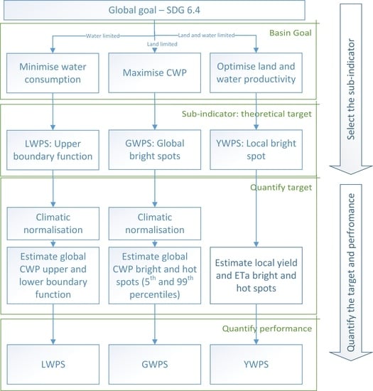
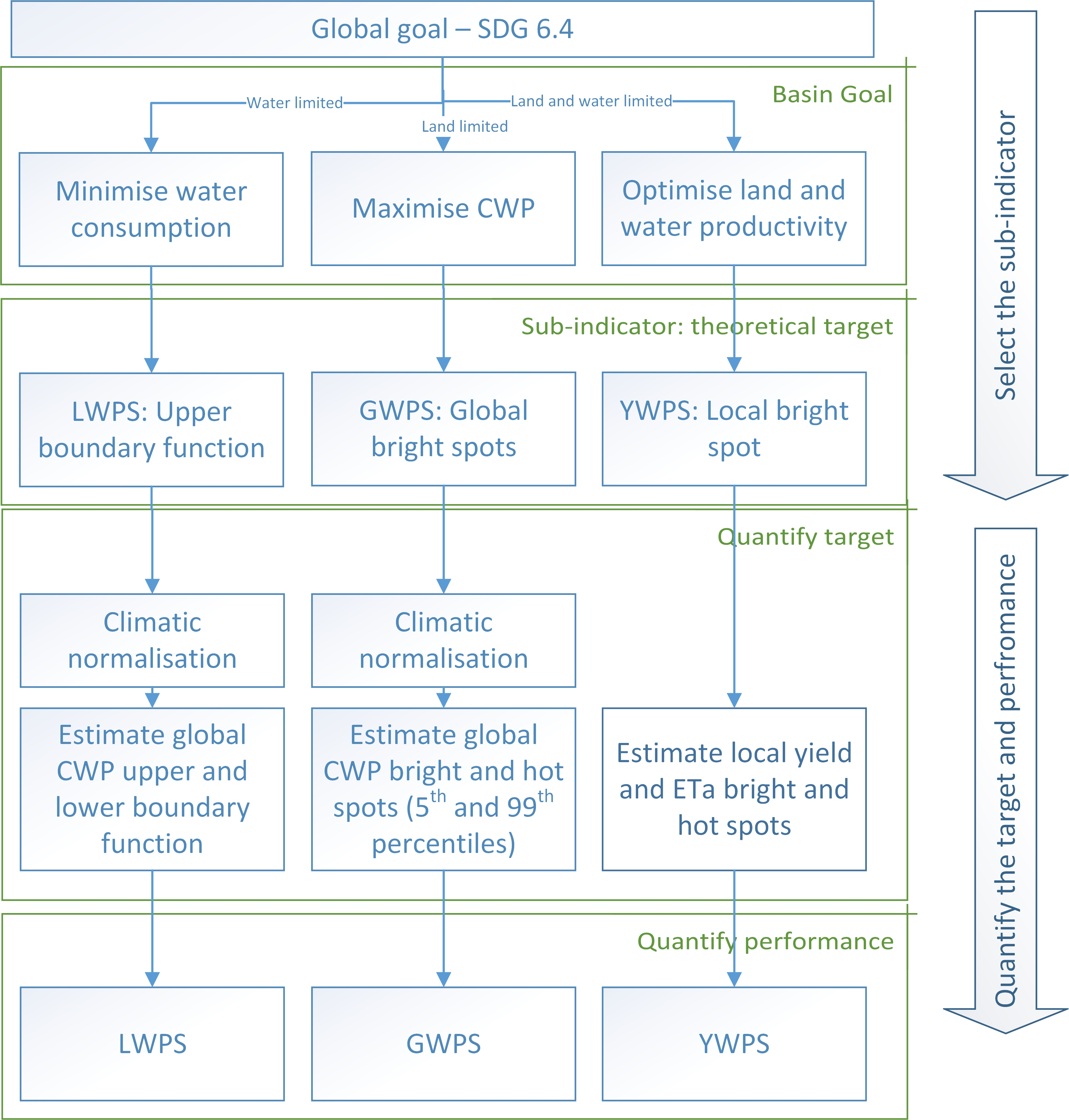
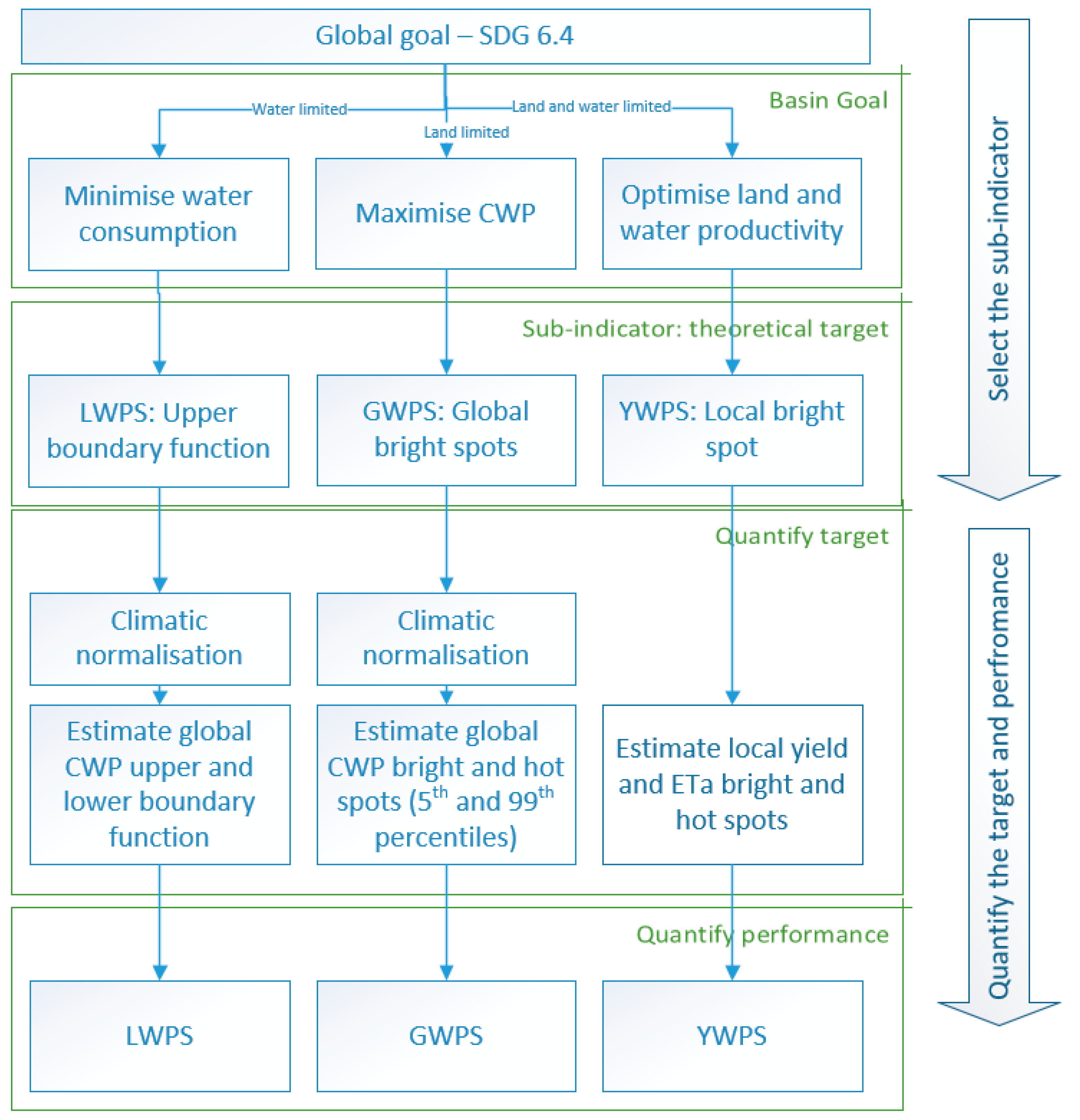
2.2. Defining a Crop Water Productivity Framework

This section will define a CWP framework around the CWP scoring methods defined in Section 2.2. The CWP framework is designed to establish the appropriate target relevant to basin needs or user defined goals.
When deciding which sub-indicator is most suitable, one first has to define the basin goals, considering ‘where are we trying to go’ and/or ‘what are we trying to achieve’. This should be defined in a more comprehensive way than simply ‘improving CWP’. Is the goal primarily to (i) move to ‘bright spots’ where a group of farmers have the highest performing CWP; (ii) improve the CWP of a specified yield zone by reaching the upper boundary function, thus focusing solely on reducing ETa; or (iii) go a step further, and identify which component of CWP, yield or ETa, has the most room for improvement? Each of the three CWP scoring methods addresses one of these goals; The GWPS addressed (i), the LWPS addresses (ii) and the YWPS address (iii). In other terms, GWPS may be preferred if the goal is to improve the overall CWP, LWPS would be preferred if the goal is to reduce overall water consumption and YWPS may be most useful to optimise both land and water productivity. Each of these scoring methods will contribute to reaching SDG 6.4, however, allow more flexibility than CWP as a sole indicator to assess performance.
The sub-indicator target, goal, ideal application, and benefits and constraints of each CWP scoring method are summarised in Table 1. The most appropriate method may also need to account for limited data, for example soils, or the absence of a local benchmark. Thus, a CWP framework should select the appropriate CWP sub-indicator dependent on both the goals specific to the basin in which it is being applied and the local constraints. The selection of the CWP sub-indicator and appropriate method will then guide the land and water management recommendations that are made. Environmental boundary delineation is specified as a possible constraint for both the GWPS and the YWPS. This is due to the lack of normalisation for soil. Although soil management practices have been shown to improve production for the same ETa [28], it has also been shown that CWP can be dramatically different between soil types within the same field [22]. These differences were related not only to soil management but soil type. Environmental boundary delineation is not included as a constraint in Table 1 as the LWPS attempt to deal with this variation through yield zones [41].
CWP or sub-indicators are tools that can be used to assess and measure the local and/or global CWP performance. The purpose of a CWP framework is to act as a support structure for the selection of CWP sub-indicators appropriate to basin needs. Thus, a generic framework, based on Table 1, to select and estimate CWP sub-indicator, is described in Figure 2. It is separated in two main components, (i) selecting the sub-indicator and (ii) applying the sub-indicator. Selecting the sub-indicator first requires definition of the basin goals, based on basin constraints. Based on this the CWP sub-indicator is selected alongside theoretical targets, i.e., bright spots or the upper boundary function. The yield, ETa and CWP or CWPc can be estimated. This provides a numerical approach to estimating the sub-indicator score and quantifying performance. Thus, once a suitable sub-indicator is identified, the appropriate numerical approach can be used first to estimate the CWP and then to quantify the target. Once the target is quantified, it can be applied to the scoring method and the performance can be assessed.
Each of the three scoring methods could in theory reference local or global targets. When applying local targets, it assumes that the local attainable CWP is being achieved, either overall, or within a yield zone. Alternatively, when global benchmarks are set, it assumes that the global target is achievable. In each CWP scoring method the target is set to a score of 10, which assumes that this correlates to the attainable CWP. Therefore, the upper thresholds dictate the CWP target. The scoring methods, as described by each CWP scoring method, therefore define the CWP targets as; (1) GWPS—when the CWPc is greater or equal to the 99th percentile global (or local) CWPc, (2) LWPS—when the CWPc is greater to or equal then the 99th percentile global (or local) CWPc in a designated yield zone and (3) YWPS—when the ETd is at the 50th percentile of the ETd and yield is greater or equal to the 99th percentile yield.

2.3. The Case Study

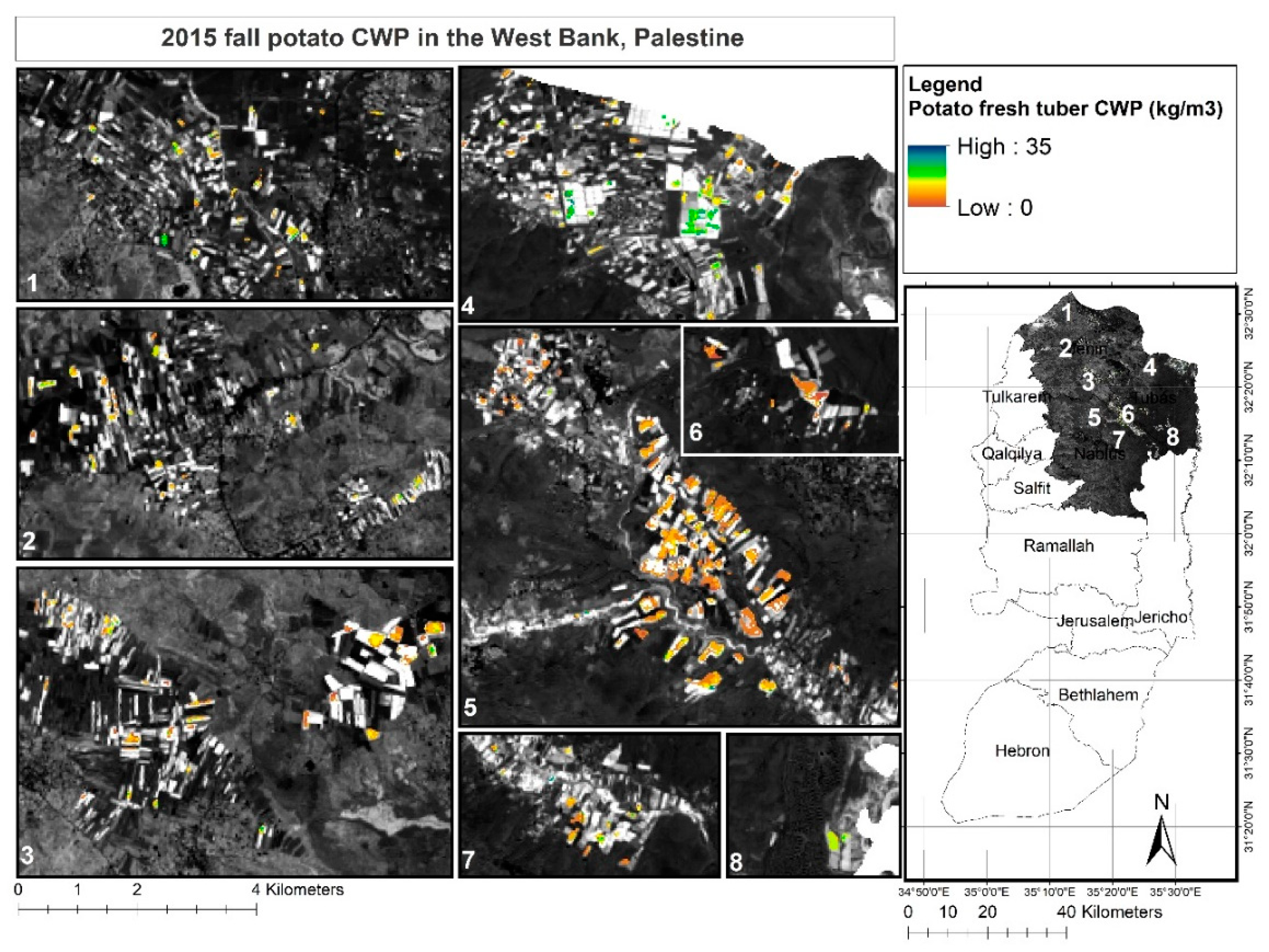
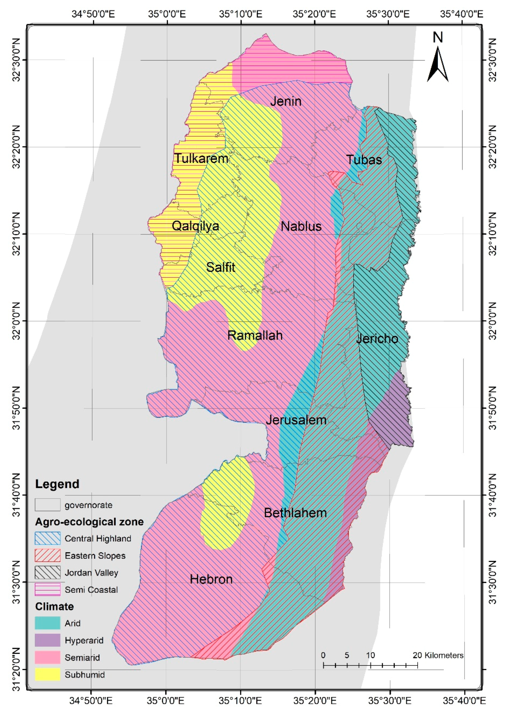
2.3.1. The Case Study, West Bank, Palestine

This paper will apply the CWP framework in the West Bank, Palestine. The West Bank is a land locked territory on the West Bank of the Jordan River that is currently facing water scarcity (Figure 3). Combined with its reliance on agriculture for both subsistence farming and economic security [48,49], this situation calls for improving water use efficiency in agriculture to ensure its sustainability and allow Palestinians to adapt to a decreasing water supply [50,51]. The West Bank is generally described as Mediterranean, which is characterised by generally cool and wet winters and long, hot and dry summers [52,53]. There are four major climatic zones in the West Bank; hyperarid, semiarid, arid and sub-humid [54] and four main agro-ecological zones; central highlands, eastern slopes, Jordan valley and semi coastal [53]. The agro-ecological zones are determined by location, rainfall and altitude. The soils of the West Bank are diverse due to the variation in climatic, parent material and topography [53]. Several authors have mapped the soils of Palestine and they have been classified into 37 classes [55]. The main classes dominating the potato growing regions are luvisols, lithosols, calcisols and grumosols. Other than grumosols, these soils are typically fairly productive.
Potato production in the West Bank is currently growing with the expansion of irrigated areas. The total area of potato production in the West Bank in 2010 was recorded at 1084 ha [48]. Approximately 95% of the potato production occurs in the Jenin, Nablus and Tubas governorates and is predominately irrigated. The average potato production was estimated, by survey, to be 34.7 ton ha−1 over the 2012–2013 and 2013–2014 season [48]. constituted approximately 71.5% of production but only occupied approximately of the 13% of the plant production area [56]. The primary irrigated crops include vegetables, citrus and bananas [49]. Olives consume occupy the most land in the regions, being approximately 47–50% of total agricultural land.
The potato crop area was estimated in this research by considering the phenological stages of the potato [57,58] and other local crops present in the same season—including cabbage [59] and onion, wheat and barley [58,60].
To assess the CWP framework in practice, three field management practices—planting season, irrigation status and crop peak—were compared. This attempts to show the implications of different basin goals, and subsequent sub-indicators, on the field, and highlight the importance of using locally relevant sub-indicators. The planting seasons compared were the 2014–2015 fall potato rotation and the 2013–2014 winter rotation. The irrigated and arable land maps were provided by the Palestinian Ministry of Agriculture [55]. The crop peak was taken as the peak normalised difference vegetation index (NDVI) on a given day of the year (DOY) for that location over the growing season, and was considered a reflection of planting date and/or crop crowing days. Under the theory of the GWPS the rotations should be directly comparable due to climatic normalisation. The distribution and break-down of each practice is defined in Table 2. Irrigated arable land is separate from Irrigated Palestinian Land, as this is land that has been converted to irrigation on within 2–3 years of the study period. Irrigated land in Israeli settlements, within in the West Bank, are also considered separately, as their irrigation practices and access are not considered to have equal status to the Palestinian farmers. Rainfed only occurs in the winter potato. All potato is irrigated in the fall.

2.3.2. Crop Water Productivity Model

The CWP components, above ground biomass production (AGBP) and ETa, were estimated in this case study using the remote sensing tool Surface Energy Balance Algorithm for Land (SEBAL) [61,62]. The yield was then estimated by considering the harvest index (HI) and the moisture content (θ) of potato:
C W P   ( k g   m 3 ) = H I A G B P ( k g   h a 1 )   ( 1 θ )   ×   10 E T a   ( m m )
The moisture content of potato, θ, was assumed to be 0.79 kg kg−1 [63], while the potato HI was taken as 0.8 [43,64]. Mean yields were validated against available data of potato production in the West Bank, Palestine.
Surface energy balance model (SEBAL), a single source model applied to visible, near-infrared and thermal infrared data. The ETa is estimated as the residual of the energy balance (latent energy) by computing the net radiation (Rn), sensible heat flux (H) and ground heat flux (G) on pixel by pixel basis. SEBAL [61,62] was selected due to its availability in Python (PySEBAL), accuracy and internalised calibration. The temporal and spatial scales are limited to the input satellite images and repeat cycle and NDVI and Ts pixel resolution. In 2009, the SEBAL algorithm for ETa, was applied and compared at field and basin levels in over 30 countries under several climatic conditions [65,66]. It has since been validated several times, with the following reported errors: daily RMSE of 0.51 mm day−1 [67] and 0.38 mm day−1 [68], seasonal error of 4.3% [69] and mean deviation of 0.06 (daily) and 0.19 (16–daily) [70].
The biomass in SEBAL is estimated based on the concept of Monteith [71], where the plant biomass is directly proportional to the photosynthetically active radiation (PAR) over the course of the growing cycle. PAR is a fraction of the incoming solar radiation (generally 45–50%) as it is a part of the short wave radiation absorbed by the plant for photosynthesis [72]. The fraction of PAR absorbed by the plant (fAPAR), or actually used by the plant, is a linear function of the normalised difference vegetation index (NDVI) [73,74]. A linear relationship between the fAPAR and NDVI from experimentally determined data derived from literature [75] is used in SEBAL. The accumulated aboveground biomass for a period is then estimated by multiplying the APAR by the light use efficiency (LUE). The LUE is scaled to account for deficiencies due to water scalar stress [75], heat stress [76] and vapour stress. The maximum LUE for C3 is set as 2.5 gMJ−1.
Further details of the SEBAL algorithm, application and validation have been described by numerous authors [62,66,68,77].
Other possible, and valid, remote sensing tools to estimate ETa for CWP include, but are not limited to; Surface Energy Balance System (SEBS) [78], Mapping EvpoTranspiration at high Resolution with Internalised Calibration (METRIC) [79] and Atmosphere-Land Exchange Inverse model (ALEXI) [80].

2.3.3. Data Requirement

The required input for SEBAL includes: visible, near-infrared and thermal infrared data—taken from Landsat 8 satellite images, a Digital Elevation Model [81] and meteorological data—taken from GLDAS [82]. The Landsat images used for the study period and the relevant potato vegetative phases are shown in Table 3.
When images were deemed not adequate, due to cloud cover, the temporal scale was increased, by multiplying the reference evapotranspiration (ET0), derived from GLDAS datasets, by the crop coefficient (kc). The crop coefficient was obtained from SEBAL, using ETa/ET0, on available dates and was then interpolated linearly [46] for missing dates. The required metrological data from GLDAS for both SEBAL input and the ET0 calculation included wind speed, relative humidity, temperature, pressure and radiation.

3. Results

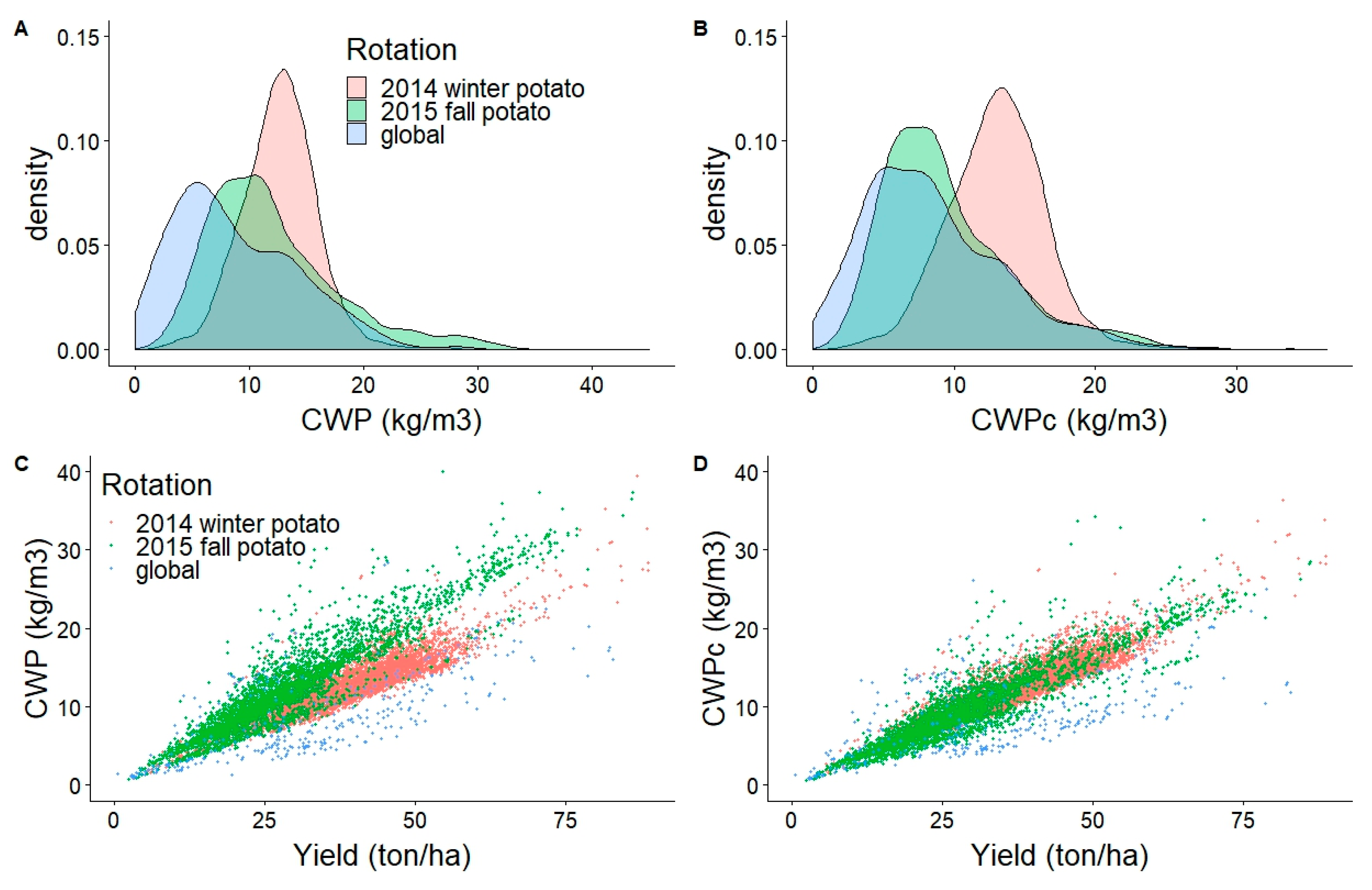
3.1. Crop Water Productivity (CWP) And Normalised CWP
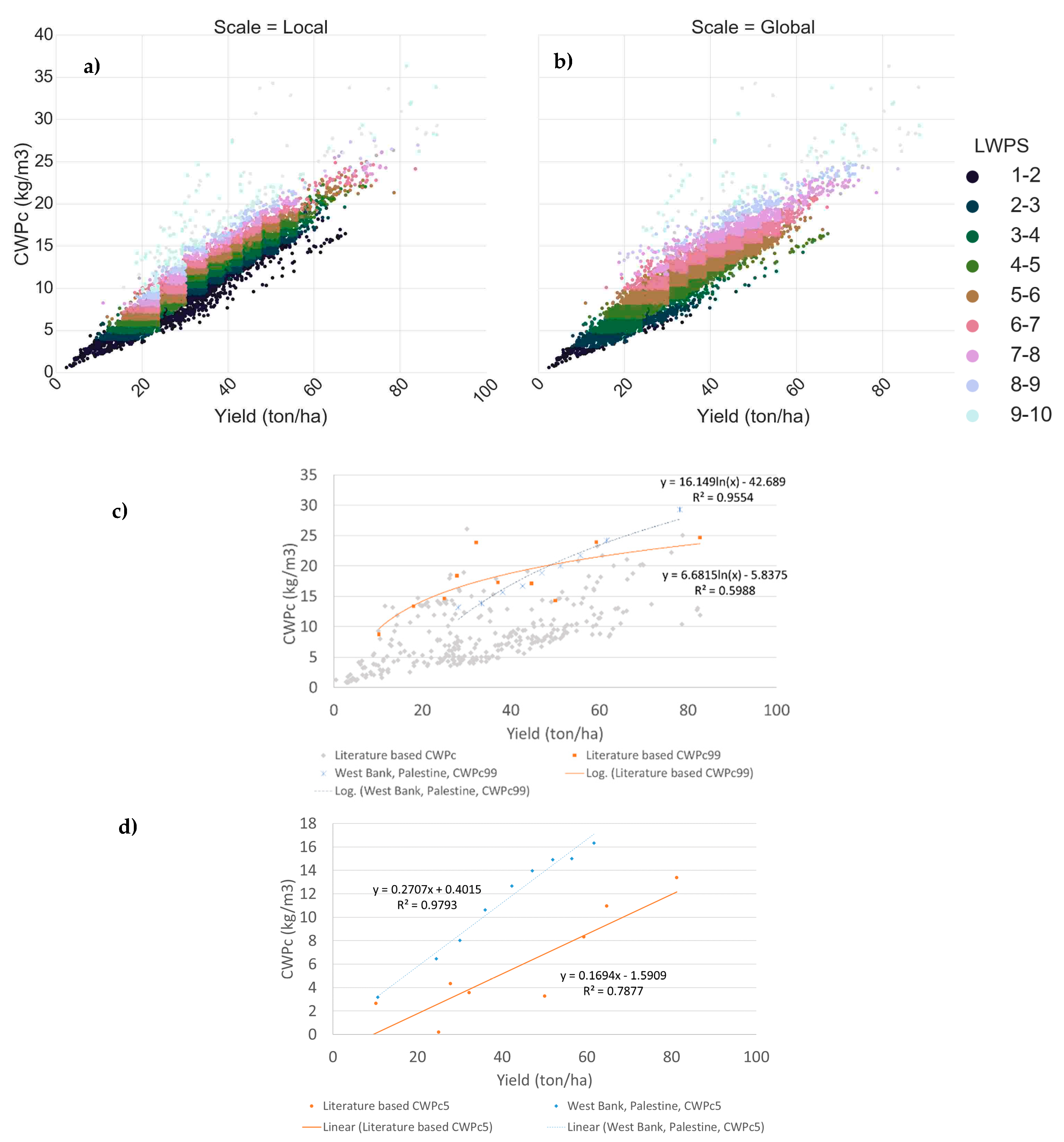
The distribution of the CWP and CWPc, along with scatter plots of the CWP and CWPc plotted against the yield, are shown in Figure 4. The results are shown for each of the rotations estimated in SEBAL in the West Bank, Palestine, and the global values compiled from literature. The distribution of winter rotation CWP and CWPc is near normal, with the highest density (mode) occurring at 13.0 kg m−3 and 13.4 kg m−3 respectively. The winter rotation has the smallest standard deviation (Table 4). The standard deviation is greater for the winter tuber CWPc as compared to the winter rotation CWP.
The global literature values and the fall rotation CWP and CWPc each have skews to the right and modes that are less than the winter rotation. This shows that the global database and the fall rotation have typically lower values than the winter rotation, which is reflected in the lower 5th percentile and mean values. However, the fall potato and global database have greater CWP distribution and greater CWP 99th percentile values than the winter rotation, with the 99th percentile values being 38% and 30% greater than the winter rotation respectively (Table 4). After normalisation the difference in 99th percentiles is almost negligible (<1.5%). The mean and modes decrease for the fall rotation and global values. The standard deviation for the global values increases.
An example of the spatial variation, the 2015 fall rotation, of the CWP is shown in
Figure 5. This map provides an example of locating the ‘bright spots’ and ‘hot spots’. The ‘bright spots’, when considering on CWP, are seen in frame 4, where the CWP is consistently high, identified by green to blue shading. Frame 5 and 6 show much lower CWP, or ‘hot spots’ with CWP frequently below the mean values (12.15 kg m3). These locations correspond to the highest values of CWP as was identified in Figure 4. This spatial identification of ‘bright spots’ and ‘hot spots’ can also be used when identifying the locations of high and low scores under each of the sub-indicators.
The impact of normalisation is further shown through the scatterplots of the CWP and CWPc plotted against the yield (Figure 4c,d). The fall and winter rotations, in particular, appear more overlaid after normalisation. Before normalisation, the fall rotation consistently shows higher CWP values being reached for a given yield, but have similar minimum values for a given yield. Conversely, after normalisation, each rotation consistently reaches similar CWPc for a given yield, while the minimum values for the fall rotation are lower. This is due to the seasonal ETa being much closer to the seasonal ET0 in the winter season. This highlights the importance of climatic normalisation, as although it appeared that the fall potato was performing similarly to the winter potato in terms of CWP, when the difference in climatic limitations of each season are taken into account the winter potato is in fact performing much better, as indicted by the CWPc.
The global CWP and CWPc values have a higher CV and a broader range of values for a given yield both before and after normalisation as compared to the West Bank CWP and CWPc values. This greater range is expected as the global values reflect a much wider and diverse range of growing conditions (including environment and management). The mean global CWP and CWPc values as derived from literature were 8.86 kg m−3 and 8.80 kg m−3 respectively. The mean values before and after normalisation were expected to be similar, as this was the case for global values of wheat, rice and maize CWP and CWPc as estimated by Bastiaanssen and Steduto 2017. While they mapped significant spatial change in CWP after normalisation the mean values and standard deviation of CWP and CWPc for each crop remained within 8% different.
In general, after normalisation there is more layover in the scatterplot with the CWPc values estimated in the West Bank. Before normalisation, the global CWP values are typically lower for a given yield, but often reach the same high CWP values at low yields (<30 ton ha−1). After normalisation, the difference between the lower global CWPc values for a given yield and the West Bank values is reduced. Simultaneously the global values are reaching higher CWPc values for a given yield and at low yields are often exceeding the local CWPc values. This suggests that the climatic normalisation was relevant in both space and time, as the climatic normalisation appeared to be successful at making the CWP more comparable in both the global setting, space, and across rotations, time.
The mean CWP values as estimated in this study, from both SEBAL and literature, are significantly greater than global studies which modelled mean potato CWP as—3.92 kg m−3 [29], 4.17 kg m−3 [32] and 4.46 kg m−3 [30,35]. However the values are comparable with those suggested by Steduto et al., (2012), who suggested typical tuber CWP values range from 4–14 kg m−3, with a dry matter content of 0.8.

CWP Validation

CWP was not validated itself, however the yield and ETa were compared to field estimates and literature. The yield of the potato was compared to the yield of 13 farmer’s plots. As farmers frequently plant in both seasons. The farmers were able to provide yield estimates for both seasons. The reported yield had a good fit with the SEBAL derived yield, with a coefficient of determination (R2) of 0.82. However, the y intercept is derived at 16.3 ton ha−1. The mean yield also compared well to the mean yields for other years as reported by ARIJ (2015). The overall mean yield estimated from SEBAL for both seasons (2014–2015) was 34.6 t ha−1 and that reported by ARIJ (2015) was 34.7 ton ha−1 (2012–2013). This is expected to reduce the representativeness at lower biomass production. No field data was available on ETa and therefore no validation of the ETa component was undertaken, however, the crop coefficient, kc (kc = ETa/ETo) was compared to literature. The estimated mean SEBAL kc was 0.85 in the fall and 0.74 in the winter rotation. The winter kc corresponds well with those reported in other literature [83,84,85] where reported kc values range from of 0.82–0.87. The winter kc was a little lower, which is a result of the higher reference evapotranspiration (ETo).

3.2. Crop Water Productivity Scores

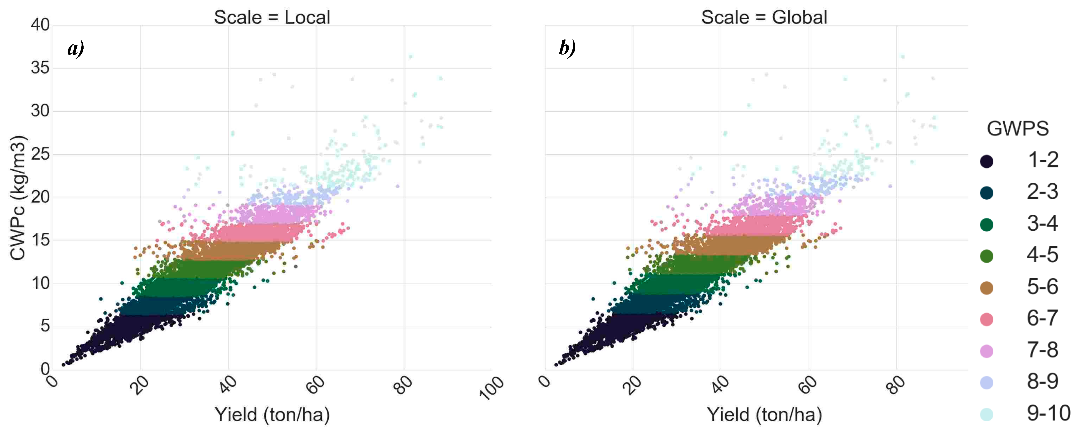
3.2.1. Global Water Productivity Score (GWPS)

The global water productivity score (GWPS) of potato in the West Bank, Palestine, is shown in Figure 6. The CWPc is on the y-axis and the yield is on the x-axis. The GWPS is shown with scores that would be assigned under a local target and global target. The local scale considers a local 99th percentile CWPc as the target, 23.54 kg m−3, while the global scale sets the global literature 99th percentile CWPc, 24.67 kg m−3, as the target (Table 2).
The difference in setting the global, as compared to local, potato CWPc as the target reduced the mean GWPS from 5.1 to 4.3. The standard deviation decreased slightly 1.91 to 2.03 and increased the coefficient of variation (CV) from 0.38 to 0.47. The difference between the local and global scales for GWPS, shown in Figure 6a,b respectively, are driven by the slightly higher overall 99th percentile CWPc identified from literature. Using the global database to define targets does not take into account cases (or crops) where there is a lack of global literature values. It also assumes that the global 99th percentile CWPc is locally attainable and that climatic normalisation is sufficient in accounting for variation in environmental conditions. Using a local target, rather than global target, applies the same numerical approach but does not require a global set of values and assumes that the local 99th percentile CWPc is equivalent to the attainable CWPc. In this case study, the global 99th percentile is being achieved locally as there are fields, approximately a combined area of 4.5 ha, with a GWPS of 10 which is seen in Figure 6.
The CWP scores for each sub-indicator are shown in Table 5. The results are shown for the GWPS using global CWP values as targets and for the LWPS using local CWP values as targets. Neither applied to the YWPS. Under the GWPS the fall rotation had only a slightly lower score than the winter rotation, 4.9 and 5.2 respectively. Before climatic normalisation the scores for each rotation was the same, 5.6, showing the impact of climatic normalisation. These scores suggest that even though the CWP of each rotation is similar, the fall rotation is not performing as well as compared to its ‘potential’. The irrigated area in Israeli settlements had the highest GWPS, 7.3. When considering only Palestinian agriculture, the rainfed potatoes have a higher score, this is despite typically lower yields. A later peak NDVI achieved a higher GWPS score for both rotations.

3.2.2. Local Water Productivity Score (LWPS)

The local water productivity score (LWPS) in relation to West Bank tuber CWPc and yield is shown in Figure 7a,b. The LWPS sets the CWPc target as the upper boundary function, which has been set to the local and global CWPc99,i for each yield zone (Figure 7c). The LWPS scores are increasing with decreasing ETa within a yield zone. The yield zones can be clearly identified by the step-like feature of the scoring method when plotted against yield. Using local potato CWPc values as the 99th percentiles to define the target results in the full breadth of scores being observed within each yield zone (Figure 7a). When the global literature 99th percentiles are used to define the upper boundary function, or the target, a variation in the range of LWPS scores within yield zone is observed (Figure 7b). The mean LWPS for the local CWP potato values as targets and the global CWP values as targets was 5.7 and 4.2 respectively. The standard deviation was 2.73 and 2.01 respectively and the CV was 0.49 and 0.48 respectively. This suggests that using global values rather than local values as the target has a greater impact in the LWPS than in the GWPS.
Figure 7c,d shows the upper and lower boundary functions of potato in the West Bank, Palestine compared to those derived from literature (Appendix A). These functions were derived by extracting the 5th and 99th percentiles per yield zone. These represent the target for each yield zone. The 5th percentile function was fitted linearly, while the 99th percentile function was fitted logarithmically. The figure shows a linear lower boundary function and a logarithmic upper boundary function (Figure 1). The local targets are lower the than the targets derived from literature up and until the yield reaches approximately 50 ton ha−1. The logarithmic regression of the upper boundary function in the West Bank has a better fit than the literature, R2 = 0.96 and R2 = 0.60 respectively. This is likely due to the small global literature database as there are less observations in each yield zone. This suggests that the upper boundary function taken from literature should evolve with the production of new datasets, and with this the upper boundary function will evolve. The lower boundary of the West Bank dataset and the global data set both show a positive linear relationship, with the West Bank lower boundary function has a higher slope (Figure 7d). The comparison of these boundary functions explain the variation in the scores between using the global and local boundary functions in that (i) In the low yield zones, the high scores are not observed as the global upper boundary function is higher than the local upper boundary function and (ii) At higher yields, the low scores are not observed due to the steeper slope of the local lower boundary function as compared to the global lower boundary function.
The upper boundary function trend, logarithm, is similar to regional scale and to global inter-comparisons as found for maize [43], wheat [86], rice [39,86] and cotton [86]. When compared to the first application of the LWPS, the upper and lower boundary functions had a better fit (higher R2) in this study [41]. While, lower boundary functions were for the most part linear for each maize, wheat and rice, the upper boundary function did not appear to be best represented by a logarithmic function.
The resulting LWPS for different management practices are different to those the under GWPS (Table 5). Under the LWPS the winter rotation had a lower score than the winter rotation, 5.9 and 5.3 respectively. The irrigation status with the highest LWPS is rainfed potato. The irrigated Israeli settlements had the lowest LWPS, suggesting the higher yields. This is because of the definition of the LWPS sub-indicator, which defines yield zones, suggesting for a given yield that the ETa is higher for irrigated Israeli settlements as compared to rainfed or Palestinian irrigated area. As compared to GWPS, the highest LWPS was for earlier peak NDVI’s.

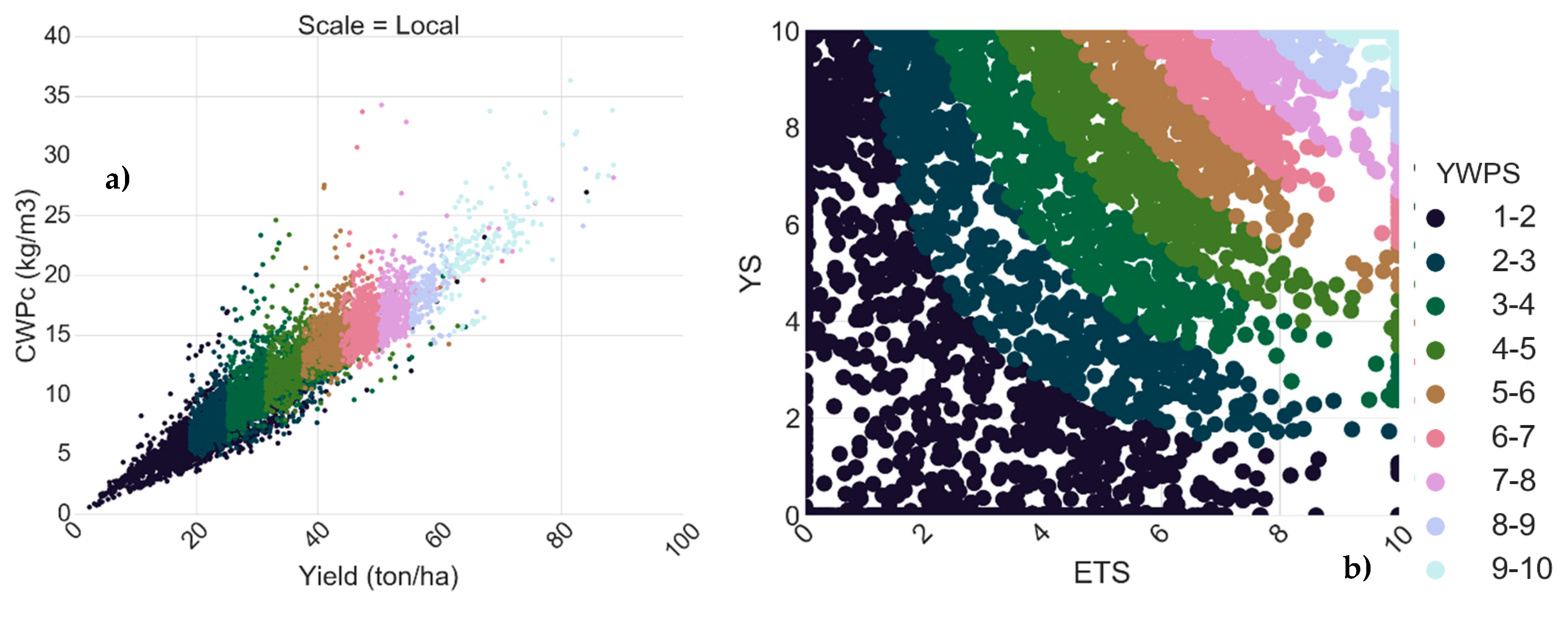
3.2.3. Land and Water Productivity Score (YWPS)

The land and water productivity score (YWPS), in relation to West Bank tuber CWPc and yield is shown in Figure 8a. The mean YWPS was 5.7 and the standard deviation and the CV was 2.6 and 0.47 respectively. The YWPS scoring method evenly weighs the yield and ETa components of CWP. This is shown in Figure 8b, where for example, an YWPS of 10 requires a YS of 10 and an ETS score of 10. This results in YWPS clusters, where multiple yields, ETa’s and CWPc’s can be represented by one score. This results in multiple YWPS for a given yield and ETa. The YWPS has used a local target. This has the benefit of ensuring the target is locally attainable. However, if this scoring method was applied to an area that was not achieving the attainable CWP, it would neglect to account for this CWP gap. A benefit of YWPS, is that the performance in each yield and the ETa’s components can quickly be identified. For example, YS of 5 means that yields are 50% of the maximum, or alternatively an ES of 10, means there is 50% ETa deficit. These fields can easily be identified when the YWPS is plotted on a YS versus ETS graph (Figure 8b). In regards to the adoption of a suitable ETd for the YWPS, the ETd of 50% did not appear to be set to low, as several fields with an ETS of 10 have obtained YS of 10.
The planting season and peak NDVI had the same order from high to low under the YWPS and the GWPS (Table 5). Under the YWPS the fall rotation had a lower score than the winter rotation, 6.4 and 4.7 respectively. The fields with a later peak NDVI had a higher YWPS as compared to those with an earlier peak NDVI. The similar mean scores between the GWPS and the YWPS arise from high scores being associated with high yields. However, variation in YWPS is seen in the distribution of scores, which is higher under the YWPS due to the designated higher weight of the ETa component. The irrigation status with the highest YWPS was irrigated Israeli settlements, 7.5. When considering only Palestinian agriculture, the Irrigated Arable Palestinian Land potatoes had the highest YWPS, 6.33.

4. Discussion

The CWP framework proposed attempts to help basins meet both local goals and SDG 6.4. While CWP as a single indicator may be a useful for the SDGs on the global setting, more specific indicators are required to ensure relevance at the local context. For the CWP framework, these have been identified as CWP sub-indicators. Each sub-indicator can help achieve different basin goals, while still contributing to SDG 6.4. This is seen not only through the sub-indicator scoring methods, or approaches, but highlighted in the variation in best management practice to achieve them.
The sub-indicator, GWPS, sets global bright spots as the target and defines the maximum attainable CWP as the target. This essentially defines the goal of improving CWP to maximise the ‘crop per drop’. This does not necessarily mean reducing water consumed by the plant, but optimising it. Therefore, total water consumption may actually increase. This was shown in the GWPS where fields with the highest GWPS frequently also had high ETa. This therefore may contradict local basin goals of minimising or reducing consumed water. The LWPS attempts to deal with this by creating the target as the upper boundary function. This is because setting the upper boundary function as the target, which is the case for the LWPS, focuses on reducing ETa within a yield zone, and could be considered to be purely focused on minimising water consumed. This may be more desirable in areas constrained by water availability rather than land [39,87], however, may contradict food security objectives, like SDG 2.4. Alternatively, YWPS, focuses on achieving the maximum CWP for the minimum ETa. This may be more suitable to a basin that is trying to optimise both land (yield) and water productivity. This was shown when the highest YWPS were associated with the maximum yield for minimum ETa.
The application of the framework in the West Bank, Palestine, showed that different management practices were associated with different scores levels under different sub-indicators. The management practices included in this research were irrigation status, rotation and planting date. The differences under each scoring system relate to the way in which the different management practices influence CWP. The planting date and season influence the CWP due to the environmental differences between seasons. For example, the fall season (fall planting date), as compared to the winter season, experiences higher rainfall and lower temperatures and is also affected by frost. These factors reduce total yield but increase water use efficiency, or CWP. Similarly, a later planting date in the fall has higher rainfall and lower temperatures as compared to earlier planting dates. Conversely, irrigation typically increases yield, as compared to rainfall, and may help maximise CWP, but does not minimise water consumption.
The highest score for a given sub-indicator suggests that, or those, management practices should be recommended. Therefore, this shows that depending on the basin goal selected, and therefore sub-indicator, different management practices would be recommended. While, this research is not trying to identify which practices are better for achieving CWP goals, it is trying to show the implications of different CWP sub-indicators in practice. The results showed that under the YWPS a winter rotation has higher performance, or mean score, under the LWPS the fall potato has a higher performance and there was little difference between rotations under the GWPS. Showing that different rotations are preferred to achieve different basin goals. Similarly, difference was seen for peak NDVI and irrigation status. For the peak NDVI, the GWPS and the YWPS a later peak NDVI has a higher performance, where and earlier peak NDVI has a higher performance under the LWPS. For the irrigation status, the Irrigated and Israeli settlements have the highest score for GWPS and YWPS, but the lowest for the LWPS. The rainfed area had the second highest scores for GWPS and LWPS, but the Irrigated Arable Palestinian Land had the second highest score for YWPS. The variation in management practices scores, associated with different sub-indicators, highlights that depending on the sub-indicator selected different attributes or farm practices may be preferred.
In cases where global targets are preferred, it must be ensured that a large enough database exists to ensure that the global 99th percentile is an accurate representation of the global potential. Due to the limited global dataset for potato, and for the application of CWP targets to other crops, it is pertinent to follow suit of previous research [34,41] and continue developing databanks of CWP, and its components, through assimilation of both remote sensing and field data. The impact was evident when setting the LWPS boundary functions. The distribution of LWPS from local potato CWPc values suggest that the CWP can be improved in all yield zones equally as each yield zone have the full distribution of scores. The distribution of LWPS from the global database CWPc values suggest that the greatest gains using the LWPS method can be gained when the yield is low, where the LWPS do not reach the maximum score and a higher number of low scores are observed, this is line with what was proposed by other authors [42].
Moving towards application of the target, or the approach to reach it, the focus then becomes where to first start targeting CWP improvements. For farmers in a higher yield zone, this may primarily be done through reducing evaporation, as the relationship between transpiration and yield are expected to be linear [88]. Alternatively, one could target farmers with both a low yield (below 50% of maximum) and low CWP, where there is the greatest room for improvement and the biggest savings could be made [42]. This is where the relationship between the transpiration and yield is not yet linear, and the improvements in marginal CWP are therefore greatest. Another alternative is to focus on improving the CWP of farmers that have both an ETS equal to 10 and a low YS, as when the ETd is greater than 0.5, small reductions in ETd can significantly increase yield. Analysis of CV may also be a useful tool to assist in targeting areas for factor analysis and CWP improvement. Where the CV is very high within a small area, the main differentiation in performance is very likely due to land and water management practices. Furthermore, in an area where the CWPc CV is low and the mean CWPc is high, it becomes important to find what land and water management practices local farmers are implementing, and if these practices are applicable to areas where the CV and mean CWP are low.
It is also important to note that the ambition of farmers often is to improve yield, while the ambitions of the basin are to reduce water consumption. As such, the desired approach defined at the basin level may conflict with that at the farm level [89]. Furthermore, it has been argued that CWP does little to improve the understanding of farm-level management [89]. This highlights the need to not only identify land and water management practices associated with high and low CWP, but the component of CWP (i.e., yield or ETa) that is being most influenced by the practice. In the context of the case study, a water limited region, the LWPS may first appear as the most suitable way to define the CWP targets. This approach may help establish methods to reduce water consumption while maintaining yields. However, the farmers typically consider their priority to be increasing yield. Their only interest in reducing water consumption is its relation to reducing pumping costs, which they specified would be redirected to methods to increase yield, such as providing additional nutrient application to the crop. If this target method is applied, additional incentives may need to be provided to encourage farmers to adopt water saving methods. Therefore, this framework is limited to the perspective of basin needs, rather than farmer needs.
This research identified that the way in which the indicator, CWP, is framed, has on the ground implications. Each sub-indicator discussed in this research can help improve CWP, and therefore move towards achieving SDG 6.4. However, the sub-indicator chosen influences ‘how’ and ‘by how much’. Therefore, while a single global CWP indicator may be preferred to monitor and assess SDG 6.4, to ensure comparability and synergy, it is too simple to identify a blanket CWP indicator. A flexible framework is required that is suitable to both the local and global setting.

5. Conclusions

This research considered multiple crop water productivity (CWP) sub-indicators, which were appropriate for both crop and region, in a CWP framework. The benefit of this, is that it defines multiple methods to improve CWP to work towards SDG 6.4, dependent on local relevance. This move beyond setting a single indicator, that may help achieve SDG 6.4, but conflict with local needs. The framework identifies that the most applicable CWP sub-indicator is dependent on the local goals. If the goal is to reduce overall water consumption, the most appropriate sub-indicator is one that aims to move farmers from a lower boundary function to an upper boundary function, of the CWP plotted against the yield—the LWPS. This, for instance, is the most relevant for areas under sever water scarcity situation such as some Middle Eastern countries where there is immediate need for curbing water consumption in agriculture. If the goal is to maximise water productivity, then a sub-indicator that targets the highest CWP is most suitable—the GWPS. If the goal is to optimise land and water productivity, then it may be more suitable to consider both land and water productivity components equally—the YWPS. Further, the basin goal and therefore subsequent sub-indicator selected determines the approach to improving CWP. If the target is the upper boundary function, the targets are reached by reducing consumed water for a given yield. If the target is the highest attainable CWP, the targets are achieved by increasing the yield at a greater rate than any associated increase in consumed water. To reach the target that weighs both land and water productivity equally, the yield would be increased without increasing consumed water or vice versa. Subsequently, the basin goal selected will dictate the land and water management practices that would be implemented. The framework developed in this research helps the user identify the sub-indicator to assess and improve performance relevant to basin goals. This allows local level consideration of SDG 6.4 without contradicting local basin needs and constraints.

Author Contributions

Conceptualization, M.L.B., W.B., P.K.; Formal Analysis, M.L.B., P.K.; Methodology, Megan Blatchford, W.G.M.B., P.K.; Validation, M.L.B.; Visualisation, M.L.B.; Writing—original draft, M.L.B.; Software, W.G.M.B.; Supervision, W.G.M.B., P.K.; Writing—review and editing, P.K., H.N.

Funding

This research was carried out under the EU funded project “Sustainable Water ActioN” (SWAN) Grant agreement NO 294947, FP7–INCO.2011–7.6 and the Palestinian Dutch Cooperation Program on Water (PADUCO) through Ebel Smidt under the TU-Delft and PADUCO partnership.

Acknowledgments

We would like to express our gratitude towards the Ministry of Agriculture (MoA) in Palestine, for their support. We would like to give special thanks to Muhannad Alhaj Hussein, who spent much time in the field, translating and providing insight, not only into water and agriculture in Palestine, but of the beauty of his culture. Also a special thanks to Issam Nofaland Jacob Keilani. This research has been possible due the financial support of the SWAN, PaDuCo project and EU funding under Experienced Water Postdoc Fellowship COFUND Programme, with particular thanks to László Hayde (SWAN) and Ebel Smidt (PaDuCo). Finally, we would like to acknowledge data obtained from the U.S Geological Survey, for the availability of Landsat 8 images.

Conflicts of Interest

The authors declare no conflict of interest.

Appendix A

Table A1. CWP and CWPc values from literature used to estimate GWPS and LWPS scores on the global scale.
LocationMin CWP (kg/m3)Max CWP (kg/m3)Median CWP (kg/m3)Median CWPc (kg/m3)nExperiment YearReference
Southern Morava, near Nis, Serbia8.129.828.707.3962008–2009[90]
Yenişehir, Bursa, Turkey2.955.574.984.63202004–2005[91]
Belgium7.8524.3615.7316.85281988–1995[92]
Gansu, China1.072.041.401.0792009–2010[93]
Tekirdag, Turkey4.699.475.824.91122003–2005[94]
Brooks, Alberta, Canada12.2819.6914.3414.00102006–2008[95]
Hebei, China11.4415.5113.4514.00112002[96]
Centraal Bekaa Valley, Lebanon7.4810.989.929.0762007–2008[97]
North of Mekelle, Ethiopia1.602.862.203.4682012[98]
Erzurum, Turkey3.876.295.655.39122003–2004[99]
Hatay, Turkey5.7814.019.8210.38162000–2002[100]
Konya, Turkey6.259.127.798.14122008–2009[101]
Quebec, Canada12.1012.1012.108.4912007[102]
Gansu, China10.8517.5313.379.94122014–2015[103]
Albacete, Spain6.5311.388.209.7782011–2012[85]
Florida, USA6.327.006.668.5022011–2012[104]
Florida, USA16.8819.3918.1322.6022012–2013[105]
Tandil, Argentina9.579.579.577.5212012–2013[106]
Gansu, China9.5716.6211.908.84182012–2013[107]
Gansu, China7.7814.3112.189.48122010–2011[108]
Shiyang River Basin, China5.8618.3713.6013.18112006–2007[109]
Gansu, China1.374.752.392.05142002–2003[110]
Idaho, USA7.388.208.208.1982006–2007[111]
Rijadh, Saudi Arabia28.0828.3428.2155.5622011–2013[112]
Orissa, India0.853.452.084.38162001–2002[113]
Bekaa Valley, Lebanon7.509.008.007.9442001[114]
Nidge, Turkey0.007.374.514.88402000–2001[115]
Iraq5.1310.267.1412.4662011[116]
Sweden16.2922.4118.7911.44152008–2009[117]

References

  1. Alexandratos, N.; Bruinsma, J. World Agriculture towards 2015/2030: The 2012 Revision; FAO: Rome, Italy, 2013; Volume 20. [Google Scholar]
  2. Steffen, W.; Broadgate, W.; Deutsch, L.; Gaffney, O.; Ludwig, C. The trajectory of the anthropocene: The great acceleration. Anthr. Rev. 2015, 2, 81–98. [Google Scholar] [CrossRef]
  3. Molden, D.J. Water for Food, Water for Life: A Comprehensive Assessment of Water Management in Agriculture; Springer: Berlin/Heidelberg, Germany, 2007; ISBN 9781844073962. [Google Scholar]
  4. Conijn, J.G.; Bindraban, P.S.; Schröder, J.J.; Jongschaap, R.E.E. Can our global food system meet food demand within planetary boundaries? Agric. Ecosyst. Environ. 2018, 251, 244–256. [Google Scholar] [CrossRef]
  5. Rockstrom, J.; Lannerstad, M.; Falkenmark, M. Assessing the water challenge of a new green revolution in developing countries. Proc. Natl. Acad. Sci. USA 2007, 104, 6253–6260. [Google Scholar] [CrossRef] [PubMed] [Green Version]
  6. Falkenmark, M.; Rockström, J.; Karlberg, L. Present and future water requirements for feeding humanity. Food Secur. 2009, 1, 59–69. [Google Scholar] [CrossRef]
  7. Hoogeveen, J.; Faurès, J.-M.; Peiser, L.; Burke, J.; van de Giesen, N. GlobWat—A global water balance model to assess water use in irrigated agriculture. Hydrol. Earth Syst. Sci. 2015, 19, 3829–3844. [Google Scholar] [CrossRef]
  8. Kijne, J.; Barron, J.; Hoff, H.; Rockström, J. Opportunities to Increase Water Productivity in Agriculture with Special Reference to Africa and South Asia; Stockholm Environment Institute, Stockholm University: Stockholm, Sweden, 2009; Volume 16, p. 48. [Google Scholar]
  9. UN-DESA. Sustainable Development Goals. Available online: https://sustainabledevelopment.un.org/sdgs (accessed on 1 May 2017).
  10. Briggs, L.J.; Shantz, H.L. Relative water requirements of plants. J. Agric. Res. 1914, 5, 116–132. [Google Scholar]
  11. Viets, F.G.J. Fertiliser and the efficient use of water. Adv. Agron. 1962, 14, 223–264. [Google Scholar]
  12. Hanks, B.J.; Tanner, C.B. Water consumption by plants as influenced by soil fertility. Agressologie 1952, 98–100. [Google Scholar]
  13. Hanks, R.J.; Gardner, H.R.; Florian, R.L. Plant growth-evapotranspiration relations for several crops in the central great plains. Agron. J. 1969, 61, 30–34. [Google Scholar] [CrossRef]
  14. Bierhuizen, J.; Slayer, R. Effect of atmospheric concentration of water vapour and CO2 in determining transpiration-photosynthesis relationships of cotton leaves. Agric. Meteorol. 1965, 2, 259–270. [Google Scholar] [CrossRef]
  15. Tanner, C.B.; Sinclair, T.R. Efficient water use in crop production: Research or re-search? Limit. Eff. Water Use Crop. Prod. 1983, 1–27. [Google Scholar] [CrossRef]
  16. Kijne, J.W.; Barker, R.; Molden, D. Improving Water Productivity in Agriculture: Editors’ Overview. Water Product. Agric. Limits Oppor. Improv. 2003, xi–xix. [Google Scholar] [CrossRef]
  17. De Wit, C. Transpiration and crop yields. Versl. Landbouwkd. Onderz. 1958, 64, 18–20. [Google Scholar]
  18. Sadras, V.O.; Grassini, P.; Steduto, P. Status of Water Use Efficiency of Main Crops; SOLAW Background Thematic Rep. TR07; FAO: Rome, Italy, 2007. [Google Scholar]
  19. French, R.; Schultz, J. Water use efficiency of wheat in a Mediterranean-type environment. I. The relation between yield, water use and climate. Aust. J. Agric. Res. 1984, 35, 743–764. [Google Scholar] [CrossRef]
  20. Ali, M.H.; Talukder, M.S.U. Increasing water productivity in crop production-A synthesis. Agric. Water Manag. 2008, 95, 1201–1213. [Google Scholar] [CrossRef]
  21. Arora, V.K.; Singh, C.B.; Sidhu, A.S.; Thind, S.S. Irrigation, tillage and mulching effects on soybean yield and water productivity in relation to soil texture. Agric. Water Manag. 2011, 98, 563–568. [Google Scholar] [CrossRef]
  22. Hatfield, J.L.; Sauer, T.J.; Prueger, J.H. Managing Soils to Achieve Greater Water Use Efficiency: A Review Managing Soils to Achieve Greater Water Use Efficiency: A Review. Agron. J. 2001, 93, 271–280. [Google Scholar] [CrossRef]
  23. Pinter, P.J.J.; Hatfield, J.L.L.; Schepers, J.S.S.; Barnes, E.M.M.; Moran, M.S.S.; Daughtry, C.S.T.S.T.; Upchurch, D.R.R. Remote sensing for crop management. Photogramm. Eng. Remote Sens. 2003, 69, 647–664. [Google Scholar] [CrossRef]
  24. Van Ittersum, M.K.; Cassman, K.G.; Grassini, P.; Wolf, J.; Tittonell, P.; Hochman, Z. Yield gap analysis with local to global relevance—A review. Field Crop. Res. 2013, 143, 4–17. [Google Scholar] [CrossRef]
  25. Rockström, J.; Barron, J. Water productivity in rainfed systems: Overview of challenges and analysis of opportunities in water scarcity prone savannahs. Irrig. Sci. 2007, 25, 299–311. [Google Scholar] [CrossRef]
  26. Allen, R.G.; Clemmens, A.J.; Burt, C.M.; Solomon, K.; O’Halloran, T. Prediction Accuracy for Projectwide Evapotranspiration Using Crop Coef cients and Reference Evapotranspiration. J. Irrig. Drain. Eng. 2005, 131, 24–36. [Google Scholar] [CrossRef]
  27. Oweis, T.; Hachum, A. 11 Improving Water Productivity in the Dry Areas of West Asia and North Africa. Water Product. Agric. Limits 2003, 1, 179. [Google Scholar]
  28. Bossio, D.; Geheb, K. Conserving Land, Protecting Water; CABI International: Oxfordshire, UK, 2008; ISBN 9781845933876. [Google Scholar]
  29. Chapagain, A.K.; Hoekstra, A.Y. Water footprint of nations. Volume 1: Main report. Value Water Res. Rep. Ser. 2004, 1, 1–80. [Google Scholar]
  30. Mekonnen, M.M.; Hoekstra, A.Y. The green, blue and grey water footprint of crops and derived crop products. Hydrol. Earth Syst. Sci. 2011, 15, 1577–1600. [Google Scholar] [CrossRef] [Green Version]
  31. Liu, J.; Williams, J.R.; Zehnder, A.J.B.; Yang, H. GEPIC—Modelling wheat yield and crop water productivity with high resolution on a global scale. Agric. Syst. 2007, 94, 478–493. [Google Scholar] [CrossRef]
  32. Siebert, S.; Döll, P. Quantifying blue and green virtual water contents in global crop production as well as potential production losses without irrigation. J. Hydrol. 2010, 384, 198–217. [Google Scholar] [CrossRef]
  33. Brauman, K.A.; Siebert, S.; Foley, J.A. Improvements in crop water productivity increase water sustainability and food security—A global analysis. Environ. Res. Lett. 2013, 8, 024030. [Google Scholar] [CrossRef]
  34. Zwart, S.J.; Bastiaanssen, W.G.M. Review of measured crop water productivity values for irrigated wheat, rice, cotton and maize. Agric. Water Manag. 2004, 69, 115–133. [Google Scholar] [CrossRef]
  35. Mekonnen, M.M.; Hoekstra, A.Y. Water footprint benchmarks for crop production: A first global assessment. Ecol. Indic. 2014, 46, 214–223. [Google Scholar] [CrossRef]
  36. Zwart, S.J.; Bastiaanssen, W.G.M.; de Fraiture, C.; Molden, D.J. A global benchmark map of water productivity for rainfed and irrigated wheat. Agric. Water Manag. 2010, 97, 1617–1627. [Google Scholar] [CrossRef]
  37. Karimi, P.; Molden, D.; Notenbaert, A.; Peden, D. Nile basin farming systems and productivity. In The Nile River Basin: Water, Agriculture, Governance and Livelihoods; Awulachew, S.B., Smakhtin, V., Molden, D., Peden, D., Eds.; Routledge-Earthscan: Abingdon, UK, 2012; pp. 133–153. [Google Scholar]
  38. Rebelo, L.; Johnston, R.; Karimi, P.; Mccornick, P.G. Determining the Dynamics of Agricultural Water Use: Cases from Asia and Africa. J. Contemp. Water Res. Educ. 2014, 153, 79–90. [Google Scholar] [CrossRef] [Green Version]
  39. Cai, X.; Molden, D.; Mainuddin, M.; Sharma, B.; Ahmad, M.-D.; Karimi, P. Producing more food with less water in a changing world: Assessment of water productivity in 10 major river basins. Water Int. 2011, 36, 42–62. [Google Scholar] [CrossRef]
  40. Cai, X.; Sharma, B.R.; Matin, M.A.; Sharma, D.; Gunasinghe, S. An Assessment of Crop Water Productivity in the Indus and Ganges River Basins: Current Status and Scope for Improvement; International Water Management Institute: Sri Lanka, South Asia, 2010; Volume 140, ISBN 9789290907350. [Google Scholar]
  41. Bastiaanssen, W.G.M.; Steduto, P. The water productivity score (WPS) at global and regional level: Methodology and first results from remote sensing measurements of wheat, rice and maize. Sci. Total Environ. 2017, 575, 595–611. [Google Scholar] [CrossRef] [PubMed]
  42. Molden, D.; Oweis, T.; Steduto, P.; Bindraban, P.; Hanjra, M.A.; Kijne, J. Improving agricultural water productivity: Between optimism and caution. Agric. Water Manag. 2010, 97, 528–535. [Google Scholar] [CrossRef]
  43. Sadras, V.O.; Cassman, K.G.G.; Grassini, P.; Hall, A.J.; Bastiaanssen, W.G.M.; Laborte, A.G.; Milne, A.E.; Sileshi, G.; Steduto, P. Yield Gap Analysis of Field Crops, Methods and Case Studies; FAO: Rome, Italy, 2015; ISBN 9789251088135. [Google Scholar]
  44. Steduto, P.; Albrizio, R. Resource use efficiency of field-grown sunflower, sorghum, wheat and chickpea: II. Water use efficiency and comparison with radiation use efficiency. Agric. For. Meteorol. 2005, 130, 269–281. [Google Scholar] [CrossRef]
  45. International Water Management Institute (IWMI). World Water and Climate Atlas; International Water Management Institute: Colombo, Sri Lanka, 2009. [Google Scholar]
  46. Allen, R.G.; Pereira, L.S.; Raes, D.; Smith, M. Crop Evapotranspiration: Guidelines for Computing Crop Requirements; FAO Irrigation and drainage paper; FAO: Rome, Italy, 1998; Volume 300. [Google Scholar]
  47. Steduto, P.; Hsiao, T.C.; Fereres, E.; Raes, D. Crop Yield Response to Water; FAO: Rome, Italy, 2012; ISBN 9789251072745. [Google Scholar]
  48. The Applied Research Institute Jerusalem (ARIJ). Palestinian Agricultural Production and Marketing between Reality and Challenges; ARIJ: Bethlehem, Palestinian, 2015; ISBN 2277722626. [Google Scholar]
  49. The Palestinian Institute for Arid Land and Environmental Studies (PIALES). Antigua and Barbuda Country Report to the FAO International Technical Conference; PIALES: Hebron, Palestinian, 1996. [Google Scholar]
  50. Attalah, N. Water for Life Water, Sanitation and Hygiene Monitoring Program (WaSH MP) 2007/2008; Palestinian Hydrology Group: Ramallah, Palestinian, 2008. [Google Scholar]
  51. The World Bank. West Bank and Gaza-Assessment of Restrictions on Palestinian Water Sector Development; The World Bank: Washington, DC, USA, 2009. [Google Scholar]
  52. United Nations Development Programme (UNDP). Climate Change Adaptation Strategy and Programme of Action for the Palestinian Authority; UNDP: New York, NY, USA, 2010. [Google Scholar]
  53. Dudeen, B. The Soils of Palestine (The West Bank and Gaza Strip) Current Status and Future Perspectives. Soil Resour. South. East. Mediterr. Ctries. 2001, 225, 203–225. [Google Scholar]
  54. Yigini, Y.; Panagos, P.; Montanarella, L. Soil Resources of Mediterranean and Caucasus Countries Extension of the European Soil Database; Office for Official Publications of the Euroean Communities: Luxembourg, 2013; ISBN 9789279303463. [Google Scholar]
  55. Ministry of Agriculture Palestine (MoA). Shapefiles Relating to the West Bank Palestine; MoA: Maastricht, The Netherlands, 2015. [Google Scholar]
  56. ARIJ. A Review of the Palestinian Agricultural Sector; ARIJ: Bethlehem, Palestinian, 2007; ISBN 9789950304031. [Google Scholar]
  57. Islam, A.S.; Bala, S.K. Assessment of Potato Phenological Characteristics Using MODIS-Derived NDVI and LAI Information. Gisci. Remote Sens. 2008, 45, 454–470. [Google Scholar] [CrossRef]
  58. González-Sanpedro, M.C.; Le Toan, T.; Moreno, J.; Kergoat, L.; Rubio, E. Seasonal variations of leaf area index of agricultural fields retrieved from Landsat data. Remote Sens. Environ. 2008, 112, 810–824. [Google Scholar] [CrossRef]
  59. Lotz, L.A.; Groeneveld, R.M.; Theunissen, J.; Van Den Broek, R.C. Yield losses of white cabbage caused by competition with clovers grown as cover crop. Neth. J. Agric. Sci. 1997, 45, 393–405. [Google Scholar]
  60. Gupta, R.K.; Prasad, T.S.; Vijayan, D. Relationship between LAI and NDVI for IRS LISS and LANDSAT TM bands. Adv. Space Res. 2000, 26, 1047–1050. [Google Scholar] [CrossRef]
  61. Bastiaanssen, W.G.M.; Meneti, M.; Feddes, R.A.; Holtslag, A.A. A remote sensing surface energy balance algorithm for land (SEBAL). 1. Formulation. J. Hydrol. 1998, 212–213, 198–212. [Google Scholar] [CrossRef]
  62. Bastiaanssen, W.G.M.; Pelgrum, H.; Wang, J.; Ma, Y.; Moreno, J.F.; Roerink, G.J.; Van Der Wal, T. A remote sensing surface energy balance algorithm for land (SEBAL): 2. Validation. J. Hydrol. 1998, 212–213, 213–229. [Google Scholar] [CrossRef]
  63. Rees, D.; Farrell, G.; Orchard, J. Crop Post-Harvest: Science and Technology: Perishables; Wiley-Blackwell: Chichester, UK, 2012; ISBN 9780632057252. [Google Scholar]
  64. Evans, L. Crop Evolution, Adaptation and Yield; Cambridge University Press: Cambridge, UK, 1993. [Google Scholar]
  65. Li, Z.L.; Tang, R.; Wan, Z.; Bi, Y.; Zhou, C.; Tang, B.; Yan, G.; Zhang, X. A review of current methodologies for regional Evapotranspiration estimation from remotely sensed data. Sensors 2009, 9, 3801–3853. [Google Scholar] [CrossRef] [PubMed]
  66. Bastiaanssen, W.G.; Noordman, E.J.; Pelgrum, H.; Davids, G.; Thoreson, B.P.; Allen, R.G. SEBAL Model with Remotely Sensed Data to Improve Water-Resources Management under Actual Field Conditions. J. Irrig. Drain. Eng. 2005, 131, 2. [Google Scholar] [CrossRef]
  67. Bala, A.; Rawat, K.S.; Misra, A.K.; Srivastava, A. Assessment and Validation of Evapotranspiration using SEBALalgorithm and Lysimeter data of IARI Agricultural Farm, India. Geocarto Int. 2015, 6049, 1–29. [Google Scholar] [CrossRef]
  68. De Teixeira, A.H.C.; Bastiaanssen, W.G.M.; Ahmad, M.D.; Bos, M.G. Reviewing SEBAL input parameters for assessing evapotranspiration and water productivity for the Low-Middle Sao Francisco River basin, Brazil. Part B: Application to the regional scale. Agric. For. Meteorol. 2009, 149, 477–490. [Google Scholar] [CrossRef]
  69. Li, H.; Zheng, L.; Lei, Y.; Li, C.; Liu, Z.; Zhang, S. Estimation of water consumption and crop water productivity of winter wheat in North China Plain using remote sensing technology. Agric. Water Manag. 2008, 95, 1271–1278. [Google Scholar] [CrossRef]
  70. Jimenez-Bello, M.A.; Castel, J.R.; Testi, L.; Intrigliolo, D.S. Assessment of a Remote Sensing Energy Balance Methodology (SEBAL) Using Different Interpolation Methods to Determine Evapotranspiration in a Citrus Orchard. IEEE J. Sel. Top. Appl. Earth Obs. Remote Sens. 2015. [Google Scholar] [CrossRef]
  71. Monteith, J.L. Solar radition and productivity in tropical ecosystems. J. Appl. Ecol. 1972, 9, 747–766. [Google Scholar] [CrossRef]
  72. Asrar, G.; Myneni, R.B.; Choudhury, B.J. Spatial heterogeneity in vegetation canopies and remote sensing of absorbed photosynthetically active radiation: A modeling study. Remote Sens. Environ. 1992, 41, 85–103. [Google Scholar] [CrossRef]
  73. Hatfield, J.L.; Asrar, G.; Kanemasu, E.T. Intercepted photosynthetically active radiation estimated by spectral reflectance. Remote Sens. Environ. 1984, 14, 65–75. [Google Scholar] [CrossRef]
  74. Wiegand, C.L.; Richardson, A.J.; Escobar, D.E.; Gerbermann, A.H. Vegetation indices in crop assessment. Remote Sens. Environ. 1991, 119, 105–119. [Google Scholar] [CrossRef]
  75. Bastiaanssen, W.G.M.; Ali, S. A new crop yield forecasting model based on satellite measurements applied across the Indus Basin, Pakistan. Science 2003, 94, 321–340. [Google Scholar] [CrossRef]
  76. Field, C.B.; Randerson, J.T.; Malmstrom, C.M. Global net primary production: Combing ecology and remote sensing. Remote Sens. Environ. 1995, 51, 74–88. [Google Scholar] [CrossRef]
  77. Allen, R.; Tasumi, M.; Trezza, R. SEBAL (Surface Energy Balance Algorithms for Land). Advanced Training and Users Manual. Idaho Implement 2002, 1–98. [Google Scholar]
  78. Su, Z. The Surface Energy Balance System (SEBS) for estimation of turbulent heat fluxes. Hydrol. Earth Syst. Sci. Discuss. 2002, 6, 85–100. [Google Scholar] [CrossRef] [Green Version]
  79. Allen, R.G.; Tasumi, M.; Trezza, R. Satellite-Based Energy Balance for Mapping Evapotranspiration with Internalized Calibration (METRIC)—Model. J. Irrig. Drain. Eng. 2007, 133, 380–394. [Google Scholar] [CrossRef]
  80. Anderson, M.C.; Kustas, W.P.; Norman, J.M.; Hain, C.R.; Mecikalski, J.R.; Schultz, L.; González-Dugo, M.P.; Cammalleri, C.; D’Urso, G.; Pimstein, A.; et al. Mapping daily evapotranspiration at field to continental scales using geostationary and polar orbiting satellite imagery. Hydrol. Earth Syst. Sci. 2011, 15, 223–239. [Google Scholar] [CrossRef] [Green Version]
  81. Jarvis, A.; Reuter, H.I.; Nelson, A.; Guevara, E. SRTM 90m Digital Elevation Database v4.1. Available online: http://www.cgiar-csi.org/data/srtm-90m-digital-elevation-database-v4-1 (accessed on 6 November 2014).
  82. Rodell, M.; Beaudoing, H. NASA/GSFC/HSL (12.01.2013) GLDAS Noah Land Surface Model L4 3 hourly 0.25 × 0.25 degree Version 2.0. 2013. (accessed on 6 November 2014).
  83. Ferreira, T.C.; Carr, M.K. V Responses of potatoes (Solanum tuberosum L.) to irrigation and nitrogen in a hot, dry climate I. Water use. Field Crop. Res. 2002, 78, 51–64. [Google Scholar] [CrossRef]
  84. De Carvalho, D.F.; da Silva, D.G.; da Rocha, H.S.; de Almeida, W.S.; da Sousa, E.S. Evapotranspiration and crop coefficient for potato in organic farming. Eng. Agric. 2013, 201–211. [Google Scholar] [CrossRef]
  85. Montoya, F.; Camargo, D.C.; Ortega, J.F.; Domínguez, A. Evaluation of Aquacrop model for a potato crop under different irrigation conditions. Agric. Water Manag. 2016, 164, 267–280. [Google Scholar] [CrossRef]
  86. Zwart, S.J. Benchmarking Water Productivity in Agriculture and the Scope for Improvement: Remote Sensing Modelling from Field to Global Scale; Delft University of Technology: Delft, The Netherlands, 2010; ISBN 9789065622372. [Google Scholar]
  87. Sari, D.K.; Ismullah, I.H.; Sulasdi, W.N.; Harto, A.B. Estimation of Water Consumption of Lowland Rice in Tropical Area based on Heterogeneous Cropping Calendar Using Remote Sensing Technology. Procedia Environ. Sci. 2013, 17, 298–307. [Google Scholar] [CrossRef]
  88. Sinclair, T.R.; Tanner, C.B.; Bennett, J.M. Water-Use Efficiency in Crop Production. Bioscience 1984, 34, 36–40. [Google Scholar] [CrossRef]
  89. Wichelns, D. Do estimates of water productivity enhance understanding of farm-level water management? Water 2014, 6, 778–795. [Google Scholar] [CrossRef]
  90. Aksic, M.; Gudzic, S.; Deletic, N.; Gudzic, N.; Stojkovic, S.; Knezevic, J. Tuber yield and evapotranspiration of potato depending on soil matric potential. Bulg. J. Agric. Sci. 2014, 20, 122–126. [Google Scholar]
  91. Ayas, S.; Korukçu, A. Water-Yield Relationships in Deficit Irrigated Potato. Ziraat Fak. Derg. 2010, 24, 23–36. [Google Scholar]
  92. Janssens, P.; Elsen, F.; Odeurs, W.; Coussement, T.; Bries, J.; Vandendriessche, H. Irrigation need and expected future water availability for potato growing in Belgium Content. Presented at the 19th Triennial Conference of the European Association for Potato Research, Brussels, Belgium, 6–11 July 2014. [Google Scholar]
  93. Zhao, H.; Wang, R.Y.; Ma, B.L.; Xiong, Y.C.; Qiang, S.C.; Wang, C.L.; Liu, C.A.; Li, F.M. Ridge-furrow with full plastic film mulching improves water use efficiency and tuber yields of potato in a semiarid rainfed ecosystem. Field Crop. Res. 2014, 161, 137–148. [Google Scholar] [CrossRef]
  94. Erdem, T.; Erdem, Y.; Orta, H.; Okursoy, H. Water-Yield Relationships of Potato Under Different Irrigation Methods and Regimens Relação Água-Produção Na Cultura Da Batata Sob Diferentes Métodos E Regimes De Irrigação. Sci. Agric. 2006, 63, 226–231. [Google Scholar] [CrossRef]
  95. Harms, T.E.; Konschuh, M.N. Water savings in irrigated potato production by varying hill-furrow or bed-furrow configuration. Agric. Water Manag. 2010, 97, 1399–1404. [Google Scholar] [CrossRef]
  96. Kang, Y.; Wang, F.X.; Liu, H.J.; Yuan, B.Z. Potato evapotranspiration and yield under different drip irrigation regimes. Irrig. Sci. 2004, 23, 133–143. [Google Scholar] [CrossRef] [Green Version]
  97. Karam, F.; Amacha, N.; Fahed, S.; EL Asmar, T.; Domínguez, A. Response of potato to full and deficit irrigation under semiarid climate: Agronomic and economic implications. Agric. Water Manag. 2014, 142, 144–151. [Google Scholar] [CrossRef]
  98. Kifle, M.; Gebretsadikan, T.G. Yield and water use efficiency of furrow irrigated potato under regulated deficit irrigation, Atsibi-Wemberta, North Ethiopia. Agric. Water Manag. 2015, 170, 133–139. [Google Scholar] [CrossRef]
  99. Kiziloglu, F.M.; Sahin, U.; Tune, T.; Diler, S. The effect of deficit irrigation on potato evapotranspiration and tuber yield under cool season and semiarid climatic conditions. J. Agron. 2006, 5, 284–288. [Google Scholar] [CrossRef]
  100. Onder, S.; Caliskan, M.E.; Onder, D.; Caliskan, S. Different irrigation methods and water stress effects on potato yield and yield components. Agric. Water Manag. 2005, 73, 73–86. [Google Scholar] [CrossRef]
  101. Yavuz, D.; Yavuz, N.; Suheri, S. Design and management of a drip irrigation system for an optimum potato yield. J. Agric. Sci. Technol. 2016, 18, 817–830. [Google Scholar]
  102. Parent, A.C.; Anctil, F. Quantifying evapotranspiration of a rainfed potato crop in South-eastern Canada using eddy covariance techniques. Agric. Water Manag. 2012, 113, 45–56. [Google Scholar] [CrossRef]
  103. Zhang, Y.L.; Wang, F.X.; Shock, C.C.; Yang, K.J.; Kang, S.Z.; Qin, J.T.; Li, S.E. Influence of different plastic film mulches and wetted soil percentages on potato grown under drip irrigation. Agric. Water Manag. 2017, 180, 160–171. [Google Scholar] [CrossRef]
  104. Reyes-Cabrera, J.; Zotarelli, L.; Dukes, M.D.; Rowland, D.L.; Sargent, S.A. Soil moisture distribution under drip irrigation and seepage for potato production. Agric. Water Manag. 2016, 169, 5–6. [Google Scholar] [CrossRef]
  105. Liao, X.; Su, Z.; Liu, G.; Zotarelli, L.; Cui, Y.; Snodgrass, C. Impact of soil moisture and temperature on potato production using seepage and center pivot irrigation. Agric. Water Manag. 2016, 165, 230–236. [Google Scholar] [CrossRef]
  106. Rodriguez, C.I.; de Galarreta, V.R.; Kruse, E.E. Analysis of water footprint of potato production in the pampean region of Argentina. J. Clean. Prod. 2015, 90, 91–96. [Google Scholar] [CrossRef]
  107. Yang, K.; Wang, F.; Shock, C.C.; Kang, S.; Huo, Z.; Song, N.; Ma, D. Potato performance as influenced by the proportion of wetted soil volume and nitrogen under drip irrigation with plastic mulch. Agric. Water Manag. 2017, 179, 260–270. [Google Scholar] [CrossRef]
  108. Qin, S.; Zhang, J.; Dai, H.; Wang, D.; Li, D. Effect of ridge–furrow and plastic-mulching planting patterns on yield formation and water movement of potato in a semi-arid area. Agric. Water Manag. 2014, 131, 87–94. [Google Scholar] [CrossRef]
  109. Hou, X.Y.; Wang, F.X.; Han, J.J.; Kang, S.Z.; Feng, S.Y. Duration of plastic mulch for potato growth under drip irrigation in an arid region of Northwest China. Agric. For. Meteorol. 2010, 150, 115–121. [Google Scholar] [CrossRef]
  110. Wang, Q.; Zhang, E.; Li, F.; Li, F. Runoff Efficiency and the Technique of Micro-water Harvesting with Ridges and Furrows, for Potato Production in Semi-arid Areas. Water Resour. Manag. 2008, 22, 1431–1443. [Google Scholar] [CrossRef]
  111. King, B.A.; Tarkalson, D.D.; Bjorneberg, D.L.; Taberna, J.P. Planting System Effect on Yield Response of Russet Norkotah to Irrigation and Nitrogen under High Intensity Sprinkler Irrigation. Am. J. Potato Res. 2011, 88, 121–134. [Google Scholar] [CrossRef]
  112. Alenazi, M.; Wahb-Allah, M.A.; Abdel-Razzak, H.S.; Ibrahim, A.A.; Alsadon, A. Water Regimes and Humic Acid Application Influences Potato Growth, Yield, Tuber Quality and Water Use Efficiency. Am. J. Potato Res. 2016, 93, 463–473. [Google Scholar] [CrossRef]
  113. Kar, G.; Kumar, A. Effects of irrigation and straw mulch on water use and tuber yield of potato in eastern India. Agric. Water Manag. 2007, 94, 109–116. [Google Scholar] [CrossRef]
  114. Darwish, T.M.; Atallah, T.W.; Hajhasan, S.; Haidar, A. Nitrogen and water use efficiency of fertigated processing potato. Agric. Water Manag. 2006, 85, 95–104. [Google Scholar] [CrossRef]
  115. Ünlü, M.; Kanber, R.; Şenyigit, U.; Diker, K. Trickle and sprinkler irrigation of potato (Solanum tuberosum L.) in the Middle Anatolian Region in Turkey. Agric. Water Manag. 2006, 79, 43–71. [Google Scholar] [CrossRef]
  116. Ati, A.S.; Iyada, D.; Najim, S.M. Water use efficiency of potato (Solanum tuberosum L.) under different irrigation methods and potassium fertilizer rates. Ann. Agric. Sci. 2012, 57, 99–103. [Google Scholar] [CrossRef]
  117. Ekelof, J.; Guamán, V.; Jensen, E.S.; Persson, P. Inter-Row Subsoiling and Irrigation Increase Starch Potato Yield, Phosphorus Use Efficiency and Quality Parameters. Potato Res. 2013, 58, 15–27. [Google Scholar] [CrossRef]
Figure 1. Conceptual approach to setting crop water productivity (CWP) targets under the global water productivity score (GWPS), local water productivity score (LWPS) and land and water productivity score (YWPS).
Ijgi 07 00414 g001
Figure 2. A CWP framework to guide the selection and estimation of CWP sub-indicators.
Ijgi 07 00414 g002
Figure 3. Governorates, climates and agro-ecological zones of the West Bank, Palestine (shapefiles provided by the Palestinian Ministry of Agriculture 2013).
Ijgi 07 00414 g003
Figure 4. (a) Density of potato fresh tuber CWP (kg m−3), (b) density of potato fresh tuber CWPc (kg m−3), (c) CWP (kg m−3) plotted against yield and (d) CWPc (kg m−3) plotted against yield. Each plot shows the winter (2014 winter rotation) and the fall (2015 fall rotation) rotations in the West Bank, Palestine, as estimated in SEBAL, and global values of CWP (global) taken from literature (Appendix A).
Ijgi 07 00414 g004
Figure 5. The spatial variation of fall (2015 fall rotation) rotation CWP in the West Bank, Palestine.
Ijgi 07 00414 g005
Figure 6. CWPc plotted against yield identifying score clusters for the GWPS setting for (a) local Palestinian 99th percentile set as the target and the (b) global 99th percentile derived from literature set as the target.
Ijgi 07 00414 g006
Figure 7. CWPc plotted against yield identifying score clusters for the local water productivity score (LWPS) for (a) local Palestinian targets and (b) based on global literature values as targets and the associated upper (c) and lower (d) boundary functions of potato CWP in West Bank, Palestine and based on global literature values.
Ijgi 07 00414 g007
Figure 8. (a) Land and water use productivity score (YWPS) in West Bank, Palestine plotted as a function of yield and CWPc and (b) YWPS plotted as a function of YS and ETS (right) for potato in the West Bank.
Ijgi 07 00414 g008
Table 1. Considerations for selecting the appropriate sub-indicator.
Aspect.Sub-Indicator
GWPSLWPSYWPS
Sub-indicator targetGlobal bright spotsUpper boundary functionLocal bright spot
Subsequent sub-indicator goalMaximise CWPReduce water consumptionMaximise land and water productivity (optimise)
Ideal applicationLand limited region/sWater limited regionWater and/or land limited region/s
BenefitsConsiders both yield and ETa improvements to meet the CWP target
Biophysical limit is target
External benchmarks not required
Does not require environmental boundary delineation
Considers both yield and ETa improvements to meet the CWP target
Identifies yield and Eta separately to target improvements
Constraints and assumptionsAssumes global attainable CWP (after normalisation) can be achieved locally.
Environmental boundary delineation may be required
Focused purely on ETa improvements.
Assumes global attainable CWP for a given yield (after normalisation) can be achieved locally.
Environmental boundary delineation may be required (normalised by yield [41])
Assumes local attainable CWP is being achieved - external benchmarks may be required
Environmental boundary delineation may be required
Climatic normalisationYesNoNo
Table 2. Fraction of irrigated and non-irrigated area in the case study.
PracticePercent of Land
Irrigation statusIrrigated Palestinian Land40.64%
Irrigated Arable Palestinian Land47.06%
Non-identified12.30%
Rainfed Palestinian Land2.39%
Irrigated and Israeli settlement0.65%
Planting seasonFall potato (2014/2015)43.73%
Winter potato (2013/2014)56.27%
Peak NDVIFall potato (2014/2015)DOY 3005.54%
DOY 33229.97%
DOY 3648.43%
Winter potato (2013/2014)DOY 06029.48%
DOY 09226.58%
Table 3. Available L8 images corresponding to selected potato rotations.
Date of Available Landsat 8 ImageDOY of Available Landsat 8 ImageApproximate Days after PlantingApproximate Vegetative Phase
2014/2015 fall potato
25 September 20142680–25Establishment
11 October 201428410–40Establishment-Stolon Initiation *
27 October 201430025–60Stolon initiation to tuber initiation
28 November 201433255–90Tuber initiation to tuber filling
30 December 201436490–120Tuber filling to maturation or harvest
31 January 2015031128Tuber maturation and harvest.
2013/2014 winter potato
27 December 20133610–30Establishment-Stolon initiation
13 February 201404450–80Stolon initiation to tuber initiation
01 March 201406060–95Stolon initiation to tuber initiation
02 April 201409280–110Tuber initiation to tuber filling
18 April 201410895–130Tuber filling to maturation or harvest
04 May 2014124110–145Tuber maturation or harvest
20 May 2014142130–160Tuber maturation or harvest.
Bold highlighting key dates for biomass production; * Stolons are stems which grow at, or just below, the ground surface.
Table 4. Potato fresh tuber CWP (kg m−3) and CWPc (kg m−3) statistics in the West Bank, Palestine, as estimated in SEBAL, and global values of CWP taken from literature (Appendix A).
ScaleSeasonMean5th Percentile99th PercentileSt.dev *CV **
CPWCWPcCPWCWPcCPWCWPcCPWCWPcCPWCWPc
West BankWinter12.6913.077.327.4322.0923.223.403.580.280.26
Fall12.159.494.843.7930.4723.545.984.650.490.49
Overall12.4511.375.714.5228.6723.434.724.490.380.40
Global8.868.801.651.8122.5124.675.416.100.610.69
* St.dev is standard deviation; ** CV is coefficient of variation.
Table 5. Mean CWP scores for different management practices using different sub-indicators.
PracticeVariationGWPSLWPSYWPS
Planting seasonFall potato (2014/2015)4.925.874.72
Winter potato (2013/2014)5.235.296.40
IrrigationIrrigated Palestinian Land4.614.784.74
Irrigated Arable Palestinian Land5.225.516.33
Rainfed Palestinian Land5.647.226.14
Irrigated and Israeli settlement7.292.667.45
Peak NDVIFall potato (2014/2015)DOY 3003.372.582.60
DOY 3324.856.464.74
DOY 3646.255.956.06
Winter potato (2013/2014)DOY 0605.126.045.80
DOY 0925.344.437.07

