Impaired Water Hazard Zones: Mapping Intersecting Environmental Health Vulnerabilities and Polluter Disproportionality


Department of Sociology, University of Oregon, Eugene, OR 97403-1291, USA
ISPRS Int. J. Geo-Inf. 2018, 7(11), 433; https://0-doi-org.brum.beds.ac.uk/10.3390/ijgi7110433
Submission received: 1 September 2018
/
Revised: 31 October 2018
/
Accepted: 4 November 2018
/
Published: 6 November 2018
(This article belongs to the Special Issue Geoprocessing in Public and Environmental Health)
Abstract
:This study advanced a rigorous spatial analysis of surface water-related environmental health vulnerabilities in the California Bay-Delta region, USA, from 2000 to 2006. It constructed a novel hazard indicator—“impaired water hazard zones’’—from regulatory estimates of extensive non-point-source (NPS) and point-source surface water pollution, per section 303(d) of the U.S. Clean Water Act. Bivariate and global logistic regression (GLR) analyses examined how established predictors of surface water health-hazard exposure vulnerability explain census block groups’ proximity to impaired water hazard zones in the Bay-Delta. GLR results indicate the spatial concentration of Black disadvantage, isolated Latinx disadvantage, low median housing values, proximate industrial water pollution levels, and proximity to the Chevron oil refinery—a disproportionate, “super emitter”, in the Bay-Delta—significantly predicted block group proximity to impaired water hazard zones. A geographically weighted logistic regression (GWLR) specification improved model fit and uncovered spatial heterogeneity in the predictors of block group proximity to impaired water hazard zones. The modal GWLR results in Oakland, California, show how major polluters beyond the Chevron refinery impair the local environment, and how isolated Latinx disadvantage was the lone positively significant population vulnerability factor. The article concludes with a discussion of its scholarly and practical implications.
1. Introduction
1.1. Background
Recent research is advancing our understanding of different manifestations of “water injustice” [1,2]. Typically, this category of environmental inequality “refers to the unequal distribution of rights to access healthy and affordable water, the lack of meaningful participation in water governance, and the misrecognition of culturally diverse ways of equitably and sustainably managing the interactions between water systems and social systems” [3] (p. 576). California’s San Francisco Bay and Sacramento—San Joaquin Delta (Bay-Delta) region (see Figure 1) has been an important site for the study of water injustice in the United States. Case studies of successive Bay-Delta water management and planning processes in the 2000s found that low-income and nonwhite people representing water justice interests were systematically excluded from those processes [4,5]. People from those same backgrounds, as well as those with limited education attainment and English-speaking ability, tend to experience heightened risk of exposure to surface water-related environmental health hazards in the Bay-Delta. The pathway to these exposure vulnerabilities include residential segregation near industrial water pollution sources [3], as well as subsistence fish consumption and low fish advisory awareness [6,7].
A recent study of the “sociospatial dimensions” of water injustice in the Bay-Delta [3] built on previous research in the region [4,5,6,7] with a cross-sectional analysis of disparate proximity to surface water toxic releases in the year 2000. Disparate proximity is manifest in the nonrandom distribution of specific social groups and environmental hazards, clustered near each other in geographic space [8]. The earlier assessment of disparate proximity to surface water toxic releases in the Bay-Delta [3] developed a novel environmental health hazard indicator—the surface water “cumulative areal-weighted modeled hazard score” (CAWMHS)—that incorporated methodological innovations of exposure assessment in the environmental inequality outcomes literature [9,10,11,12,13]. Surface water CAWMHS models the relative health hazard posed to census geographies given their proximity to surface water toxic release facilities with data from the U.S. Environmental Protection Agency’s (EPA) Risk-Screening Environmental Indicators (RSEI) database, version 2.3 [14]. The RSEI database attaches health-related hazard information to toxic releases that are self-reported by manufacturing facilities with more than 10 employees to the U.S. EPA’s Toxic Release Inventory (TRI).
The previous assessment of the sociospatial dimensions of water injustice in the Bay-Delta focused on the intersecting environmental health vulnerabilities associated with disparate proximity to surface water CAWMHS in the region [3]. Importing insights from the sociological study of intersectionality [15,16], intersectional environmental inequality outcomes research of that kind focuses on how the spatial concentration of individuals identifying with multiple social identities is associated with disparate proximity or unequal exposure to environmental hazards [17,18,19,20]. The benefit of this approach is that it moves beyond the classic environmental inequality debates over race and class, for example, to a view on how different low-income racial groups experience segregation and environmental health hazard exposure [19]. This intersectional approach also accords with survey research on racial differences in hazardous subsistence fish consumption rates among the economically disadvantaged and those with limited English-speaking ability in the Bay-Delta [6,7]. Previous research [3] found that factor variables representing the spatial concentration of “Black disadvantage” (i.e., poor Blacks and Blacks without a high school diploma) and “isolated Latino disadvantage” (i.e., poor Latinos, Latinos without a high school diploma, and primarily Spanish-speaking households) were statistically significant and positive predictors of block group exposure to surface water CAWMHS, net of other factors.
There were two other significant, negative predictors of block group-level surface water CAWMHS in the Bay-Delta: Median housing values and proximity to the Chevron oil refinery in Richmond, California [3]. The negative association between housing values and environmental hazard exposure is fairly consistent in the environmental inequality outcomes literature [20,21]. It also accords with expectations in the broader social science literature on uneven development, which focuses on how the unequal spatial distribution of economic resources influences the health and wellbeing of people and places [22,23]. Proximity to the Richmond Chevron oil refinery was treated as a statistical control to account for the spatial clustering of surface water CAWMHS near this facility, which was the most hazardous industrial polluter in the region [3].
1.2. Objectives and Hypotheses
The present study addresses three limitations in previous research on the sociospatial dimensions of surface water-related environmental health vulnerabilities within the Bay-Delta region [3]. First, surface water CAWMHS only includes industrial surface water toxic releases from the U.S. EPA RSEI database. In addition, surface water CAWMHS does not account for the fate and transport of pollutants as found in a number of hydrological analyses used for assessing total maximum daily loads (TMDL) for U.S. waterways [24,25,26,27,28,29]. Accordingly, questions remain regarding the unequal spatial distribution of a broader set of point and non-point-sources (NPS) in the region. Such sources are identified in lists of “impaired water bodies,” which are maintained by states (e.g., California), per section 303(d) of the U.S. Clean Water Act, and are subject to review by the U.S. EPA.
The 303(d) list of impaired waters represents waters that state agencies expect to violate water quality standards. These expected violations occur despite the regime of federal technology-based regulatory controls and permitting systems for point source discharges, such as those from manufacturing facilities in the National Pollutant Discharge Elimination System. NPS discharges are important contributors to water impairment beyond these point sources, but they are not under direct federal jurisdiction. NPS discharges typically include urban runoff, agricultural pollution sources, wastewater, and the lingering effects of historical resource extraction and massive water engineering projects. The goal of the 303(d) list is to identify the point source and NPS pollutants present in any given water body that lead to water quality violations then use a variety of strategies, particularly the TMDL program, to create what is essentially a state-negotiated, federally-approved, permitted budget for specific contaminant-source combinations [30]. The TMDL program has risen to prominence recently with the U.S. EPA approving more than 37,000 pollutant- and water-body-specific TMDLs between 2009 and 2012 [31].
In this study, I address the limited focus on industrial point-source hazards as a dependent variable in previous research on the Bay-Delta [3]. I move beyond this focus using geographic information systems (GIS) to create a new environmental health hazard indicator—“impaired water hazard zones’’—from California’s 303(d) list of impaired waters for 2006. I used the impaired water list from 2006 to maintain temporal comparability with data from 2000 that was used in previous research [3]. In so doing, I test three hypotheses derived from literature reviewed above regarding the intersecting population vulnerability and uneven development factors that are associated with unequal risk of exposure to surface water-related health hazards in the Bay-Delta. In one of these hypotheses—and throughout the remainder of this article—I deviate from earlier work on the Bay-Delta [3] and use the gender-neutral term, “Latinx,” to refer to individuals that are typically identified as “Hispanic” or with the gendered term, “Latino” [32]. The first set of hypotheses tested in this study are as follows:
Hypothesis 1 (H1):
The Black disadvantage hypothesis states that the spatial concentration of socioeconomically disadvantaged Blacks will be positively associated with block group proximity to impaired water hazard zones, net of other factors.
Hypothesis 2 (H2):
The isolated Latinx disadvantage hypothesis states that the spatial concentration of socioeconomically disadvantaged Latinxs and primarily Spanish-speaking households will be positively associated with block group proximity to impaired water hazard zones, net of other factors.
Hypothesis 3 (H3):
The uneven development hypothesis states that housing values will be positively associated with block group proximity to impaired water hazard zones, net of other factors. That is, low housing values will be associated with block group proximity to impaired water hazard zones.
This study also develops an alternative conceptual framework than used in previous research [3], which reconsiders the continuing significance of contemporary industrial sources of water injustice in the Bay-Delta. In particular, it charts deeper connections between the sociospatial dimensions of water injustice and the environmental-sociological literature on “disproportionality”. The disproportionality perspective focuses on two ways in which power and privilege intertwine to produce unequal environmental health vulnerabilities. The first dimension involves dominant social actors’ “privileged access” to pollute or otherwise manipulate the biophysical environment to suit their interests [33]. Privileged access is legitimated through taken for granted or “privileged accounts”, which shift regulatory and public scrutiny away from the polluting activity of dominant actors [33]. The present study focuses on privileged access by examining “polluter disproportionality”, which refers to the disproportionate share of environmental pollution (and their associated health implications) from a small number of industrial producers [34,35,36,37].
From the disproportionality perspective, the significance of disparate proximity to the Chevron oil refinery in Richmond is more than a mere control variable to account for the spatial clustering of surface water-related health hazards in the Bay-Delta, as found in previous research [3]. Instead, proximity to the Chevron refinery is an indicator of how marginalized communities, such as Richmond, California and its neighbors [38,39], face significant environmental health threats from neighboring “super emitters” [37] like Chevron. Indeed, Chevron and other major oil and gas producers have gone to considerable lengths to challenge U.S. environmental law [40] and local protests to secure “privileged access” to disproportionately pollute the biophysical environment of vulnerable communities throughout the world [41,42,43,44,45,46,47,48,49].
The disproportionality perspective aligns with various components of critical physical geography. Critical physical geography is committed to rigorously examining the material dimensions of biophysical landscapes. Akin to intersectionality studies, critical physical geography is also centrally concerned with exposing how human actions and multiple and sometimes intersecting social inequalities (e.g., race, class, and/or linguistic ability) impact people’s experience of the biophysical environment with implications for their health and wellbeing [50,51]. For example, McClintock [23,52] found unequal concentrations of soil lead contamination and elevated childhood blood lead levels in Oakland, California’s flatland areas, which are predominantly nonwhite, low-income, industrial, and filled with pre-1940s housing stock. McClintock’s [23] historical study of Oakland revealed how its unequal landscape of environmental health vulnerabilities is linked to a series of exclusionary land use controls (i.e., racially-restrictive covenants), uneven development, and corporate advocacy and regulatory acquiescence for the pervasive use of lead-based products, especially lead-based gas and paint. The remnants of these lead-based environmental health hazards, despite their subsequent ban, are found in the soils of Oakland’s nonwhite, low-income, and industrial neighborhoods that have been neglected while capital investment and redevelopment unfold elsewhere in the hills and suburbs surrounding Oakland [23].
The regression analyses featured in this study test two additional hypothesis. They derive from previous empirical findings [3], the disproportionality perspective in environmental sociology [33,34,35,36,37], and the general framework of critical physical geography [23,50,51,52]. Importantly, these hypotheses explicitly distinguish the effects of proximate cumulative industrial pollution sources, as represented in the surface water CAWMHS, from proximity to the Richmond Chevron oil refinery. Doing so helps to isolate the disproportionate effects that super emitters with privileged access to the environment have on the sociospatial dimensions of water injustice in the Bay-Delta. In testing the following hypotheses, I incorporate the U.S. EPA RSEI data from 2000 to 2006 to develop an updated indicator of surface water CAWMHS than was found in the previous research [3]:
Hypothesis 4 (H4):
The industrial point source pollution hypothesis states that surface water CAWMHS will be positively associated with block group proximity to impaired water hazard zones, net of other factors.
Hypothesis 5 (H5):
The super emitter hypothesis states that proximity to the Richmond Chevron oil refinery will be positively associated with block group proximity to impaired water hazard zones, net of other factors. That is, block groups near the Richmond Chevron oil refinery will also be near impaired water hazard zones.
Third, this study attends to the spatial non-stationarity of intersecting environmental health vulnerabilities and polluter disproportionality that has yet to be examined in previous research. Spatial non-stationarity in this context refers to how relationships between variables examined at one spatial scale (e.g., the census block group) using the same method of assessing exposure can vary across different geographic extents (e.g., the regional versus sub-regional scale) [53]. Since the introduction of geographically weighted regression (GWR) techniques [54,55], studies have used GWR to model spatial non-stationarity in a wide variety of multivariate statistical relationships. These include applications of geographically weighted logistic regression (GWLR) to model local variation in the predictors of binary outcomes spanning multiple subfields in human and physical geography [56,57,58,59,60,61,62,63,64,65,66,67,68]. Within the environmental inequality outcomes literature, spatial non-stationarity has been identified in the aggregate-level population vulnerability predictors of industrial air-toxic releases in New Jersey, USA [69], estimated lifetime cancer risk from cumulative ambient air-toxic pollution in Florida, USA [70], and vegetation land cover in shrinking and growing US cities [71]. GWR-based environmental inequality outcomes research has also uncovered spatial non-stationarity in the effect of particulate matter and other environmental exposures on adverse childhood respiratory conditions in the United Kingdom [72] and in the USA [73]. Given these insights, the present study tests the following hypothesis regarding the predictors of disparate proximity to impaired water hazard zones in the Bay-Delta:
Hypothesis 6 (H6):
The spatial non-stationarity hypothesis states that the relationship between intersecting population vulnerability, uneven development, proximate industrial point source pollution levels and sources, and block group proximity to impaired water hazard zones will vary significantly at the block group level throughout the Bay-Delta region.
This study is the first to couple global logistic regression (GLR) with GWLR to analyze the extent of spatial non-stationarity in the relationship between intersecting population vulnerability factors, uneven development, polluter disproportionality, and a binary environmental inequality outcome (in this case, block group proximity to impaired water hazard zones). It used GLR to test the hypotheses presented above regarding the predictors of census block groups’ proximity to impaired water hazard zones throughout the Bay-Delta. The results from those analyses support previous research on the sociospatial dimensions of water injustice in the Bay-Delta [3]. However, the GWLR specification improved model fit and uncovered spatial non-stationarity in the predictors of block group proximity to impaired water hazard zones. As illustrated in the modal GWLR results in Oakland, California, other industrial polluters (beyond the Richmond Chevron refinery) adversely affect the local environment. Further, isolated Latinx disadvantage, rather than Black disadvantage, was the sole positively significant intersecting population vulnerability predictor of census block groups’ proximity to impaired water hazard zones. The article closes with a discussion of its future scholarly and practical implications in light of these findings.
2. Materials and Methods
This study applies the interdisciplinary, critical physical geography “methodological four-square” [51] to the analysis of impaired water hazard zones, as summarized in Figure 2. In testing the six guiding hypotheses of this study, I draw on quantitative methods from (1) the biophysical sciences to guide my spatial analysis of surface water health hazards (Box A, Figure 2), and (2) the social sciences in my spatial analysis of intersecting environmental health vulnerabilities and their sources (Box B, Figure 2). I supplement that quantitative approach with a qualitative, narrative description of (1) surface water pollutants and their hazard levels (Box C, Figure 2); and (2) the anthropogenic and biophysical sources of surface water pollutants (Box D, Figure 2). The remainder of this section is primarily devoted to explaining the quantitative methods used in this study.
2.1. Unit of Analysis
Census block groups defined for the year 2000 are the unit of analysis in this study. These areal units, produced by the U.S. Census, typically span contiguous areas that aggregate census blocks and contain between 600 and 3000 people. A benefit of using these units for the year 2000 is that doing so maintains comparability between the present study and previous research on the sociospatial dimensions of water injustice in the Bay-Delta [3]. In addition, census block groups are the smallest unit of analysis for all data included in this study, and they provide more precision in population exposure estimates than is possible with higher levels of aggregation, such as census tracts.
2.2. Dependent Variable
This study’s dependent variable is a binary measure of census block group proximity to impaired water hazard zones in the Bay-Delta (1 = yes; 0 = no). Measuring proximity to an environmental hazard is a crude measure for exposure in environmental inequality studies [10]. However, the proximity approach is advocated because: (1) Research suggests there are psychological, community health, and economic risks from being proximate to an environmental hazard [74,75]; and (2) proximity is one of the best proxies available when unable to assess actual exposure [10,11]. Under these assumptions, research on air- [21,76] and land-based [11] environmental hazards typically use critical distances between one and three miles to a hazard in assessments of disparate proximity.
A related approach is suggested for surface water hazards. The U.S. EPA determined the 6.4-km (4-mile) distance to surface water hazards to be the “inner zone”, or plausible exposure zone, to surface water hazards for its Hazard Ranking System for National Priority List sites [3,13]. I adapted these guidelines for the present study by using ArcMap 10.4 to draw 6.4-km buffers around water bodies identified in the 2006, 303(d), impaired water bodies list for California. Data on the impaired water bodies were derived from the California State Water Resources Control Board’s (SWRCB) list of impaired water bodies for 2006 [77,78]. I then intersected these buffers to construct the impaired water hazard zones. These zones, shown in Figure 3, Map C, represent spaces that are simultaneously within the 6.4-km plausible exposure zones to 37 segments of impaired minor water bodies (i.e., “rivers, streams, and coastal shorelines”) (see Figure 3, Map A) and 69 segments of major water bodies (i.e., “bays, harbors, estuaries, lakes, reservoirs, and tidal wetlands”) (see Figure 3, Map B). This spatial analytic strategy provides a crude measure of census block group plausible exposure to surface waters that were significantly polluted from point sources and NPS in the Bay-Delta as of 2006.
As described in Section 3.1.1, the impaired water bodies analyzed in this study represent the historical accumulation of a multiplicity of point and NPS pollutants in the surface waters of the Bay-Delta. I assessed the disparate proximity of census block groups to impaired water hazard zones with the commonly used “50 percent areal containment method” [3,10,11]. In the context of the present study, this method involved calculating the extent to which at least 50 percent of a census block group’s area intersected the impaired water hazard zones. Similar to previous research [3,10,11], I found this approach produced less variation in the size of block groups contained in the impaired water hazard zones than the comparable distance-based, boundary intersection method. The mean area of the 1637 block groups meeting the 50 percent areal containment threshold was 2.33 square kilometers (0.90 square miles) (SD = 13.55 square kilometers/5.13 square miles). The mean area of the 1848 block groups meeting the boundary intersection threshold was 4.98 square kilometers (1.92 square miles) (SD = 27.21 square kilometers/10.51 square miles).
2.3. Independent Variables
2.3.1. Intersecting Population Vulnerability Factors
I used two factor variables—Black disadvantage and isolated Latinx disadvantage—to maintain comparability with previous research [3] and to test the Black disadvantage (H1) and isolated Latinx disadvantage (H2) hypotheses stated above. Each factor represents “structural factors” of environmental health vulnerability [68] that are salient in the Bay-Delta water environment [3,4,5,6,7]. These include poverty, limited educational attainment, and limited English-speaking ability, which are uniquely correlated with each racial group at the census block group level. Specifically, Black disadvantage, is composed of the percent of individuals whose 1999 income was below the federal poverty level and the percent of individuals 25 years and over without a high school diploma that identified as Black. Isolated Latinx disadvantage includes similar poverty and low educational attainment measures for those identified as “Latino” or “Hispanic” in the 2000 census. However, it also includes the percent of households who are linguistically isolated and are Spanish-speaking. “Linguistically isolated households” are those in “which all members 14 years old and over speak a non-English language and also speak English less than ‘very well’ (have difficulty with English)” [79] (p. B-32).
These factor variables were constructed with separate Principal Component Analyses (PCAs) from summary file 1 and 3 from the 2000 U.S. Census [3]. Each PCA produced unrotated factor solutions, which were extracted by analyzing correlations between each component variable. This involved using a maximum of 25 iterations, eigenvalues greater than 1.00, and listwise deletion for block groups with missing values. The final factor scores are the standardized linear combination of loading weights for each component produced with a regression method. Estimating the total variance explained by each factor component informed validity assessments of each factor. The reliability of the factor results were assessed with Cronbach’s alpha scores calculated from additional scale analyses.
Table 1 displays the reproduced PCA results for the two factor variables that were used in previous research [3]. Those PCA results indicate the factors have high validity and reliability. The percent of variance explained in the factor components ranged from 84.08 for isolated Latinx disadvantage to 90.46 for Black disadvantage. Similarly, the Cronbach’s alpha scores for the factors ranged from 0.862 for isolated Latinx disadvantage to 0.892 for Black disadvantage. The factor loadings for each factor were all greater than or equal to 0.882. Figure 4 and Figure 5 present the spatial distribution of the two intersecting population vulnerability factor variables. As shown in Figure 4, Black disadvantage levels were mostly elevated in or near the urban centers of Sacramento, Alameda, and San Joaquin Counties. Figure 5 illustrates how isolated Latinx disadvantage levels were elevated in the central section of the region in addition to its urban centers of Sacramento, Alameda, and San Joaquin Counties.
2.3.2. Uneven Development
Housing values are an aggregate-level indicator of uneven development [22]. They are also used as indicators of environmental health vulnerability in the U.S. [19,20,21], and to surface water hazards in the Bay-Delta [3]. Following previous research [3,20,21], I operationalized housing values as a ratio of block group-to-county median housing values in 2000. For brevity, I refer to this variable as relative median housing value. I use this variable in my test of the uneven development hypothesis (H3). Figure 6 presents the spatial distribution of relative median housing value. An emergent theme from Figure 4, Figure 5 and Figure 6 is that Black disadvantage and isolated Latinx disadvantage overlapped in the Bay-Delta region’s urban centers and to some extent in the center of the region. In addition, many, but not all, of these spaces also had low relative median housing values.
2.3.3. Contemporary Industrial Pollution Sources
I used an adapted measurement of the surface water CAWMHS [3] in my test of the industrial point source pollution hypothesis (H5). From the RSEI database [14], I selected all facilities that were within 6.4 km from the six-county Bay-Delta region and that released toxins directly into the surface waters (release code = 3) of the region from 2000 to 2006. The 6.4-km proximity threshold maintains consistency with the 6.4-km plausible exposure zone used to construct the impaired water hazard zones. The 2000–2006 period provides an updated assessment of the environmental health hazard associated with surface water toxic releases from the 2000 snapshot used in earlier research [3]. This period also matches this study’s analysis of impaired waters in the Bay-Delta in 2006. I found that 51 facilities within 6.4 km of the Bay-Delta released toxins into the region’s surface waters from 2000 to 2006 and had available data within the RSEI database [14] to calculate the relative health hazard of those toxic releases.
The modeled hazard scores for these surface water toxic releases were initially calculated in the RSEI database by multiplying the pounds of toxic releases with their chemical-specific oral toxicity weights [14] (pp. 14–15, 119, 163). The hazard scores do not incorporate the transport and fate of chemicals and dose-response effects for proximate populations [12,14]. However, the benefit in using the hazard scores is that they are not population-weighted. Accordingly, they mitigate against inflated estimates of the association between the demographic composition of census geographies and proximate environmental health hazard levels [3,12].
The RSEI-based modeled hazard scores are not associated with proximate census geographies. Accordingly, I used the following equation to calculate the surface water CAWMHS for 2000 to 2006 for census block groups within the Bay-Delta:
where y is surface water CAWMHS, H is the surface water modeled hazard score from the RSEI database for surface water toxic releases from facility t, P is the proportion of area for block group i that intersected the 6.4 km buffer to facility t, and A is the total area for block group i [3].
However, in contrast to previous research [3], I used the boundary intersection method [11] to code census block groups as proximate to surface water toxic releases if any of their boundaries intersect the 6.4-km plausible exposure zone buffer to industrial facilities that released toxins directly into the Bay-Delta surface waters from 2000 to 2006. This deviation from previous work is based on this study’s objective of using a wider geographic search parameter to test the industrial point source pollution hypothesis (H5) and to model the relative environmental health hazard of proximate surface water toxic releases for block groups that may also contribute to block groups being contained within the impaired water hazard zones. Thus, the surface water CAWMHS for 2000 to 2006 in the present study was created for block groups who intersected the 6.4-km surface water toxic release facility buffer. It was calculated by multiplying the surface water modeled hazard score for a given facility by the proportion of block group square meters that intersected the buffer to each facility, summing those scores for each block group, and dividing that sum by the block group area. In my test of the industrial point source pollution hypothesis, I use surface water CAWMHS, 2000–2006, in hundreds of thousands (i.e., the 2000–2006 surface water CAWMHS divided by 100,000). I do so because of the large raw values for this variable, and the effect of surface water CAWMHS on the likelihood of block group 50 percent areal containment in an impaired water hazard zone is more evident in 100,000 units than in units of one.
Map A in Figure 7 displays the resulting spatial distribution of surface water CAWMHS from the 51 facilities that released surface water toxins in the Bay-Delta region from 2000 to 2006. That spatial distribution overlaps to some extent with the spatial distribution of nonwhite disadvantage and median housing values shown throughout the region in Figure 4, Figure 5 and Figure 6. It also shows the Chevron terminal stations to illustrate the hazardous reach that Chevron’s oil and gas production and distribution activities have throughout the region beyond its oil refinery in Richmond. Indeed, when one adds in the RSEI modeled hazard score of the Chevron terminal stations to that of its oil refinery, Chevron’s four facilities were responsible for 77.78 percent of the 259,084,979.66 modeled hazard score of the combined surface water toxins from the 51 facilities.
Map B in Figure 7 visualizes the 6.4-km facility buffers used to calculate the 2000−2006 surface water CAWMHS in the context of the Richmond and Berkeley, California area. It illustrates that the Chevron oil refinery was not the lone emitter in that area, which was also the case in 2000 [3]. The 2000−2006 surface water CAWMHS helps to account for the spatial concentration of this cumulative impact of multiple industrial point pollution sources. Nonetheless, the RSEI-based surface water modeled hazard score for the Chevron oil refinery was 118.17-times more hazardous than the combined RSEI-based surface water modeled hazard score for the four other facilities, as shown in Figure 7, Map B. The new empirical details about the disproportionately high hazard levels of the Richmond Chevron oil refinery’s surface toxic releases from 2000 to 2006 accord with the disproportionality framework presented in Section 1.2. Accordingly, the final independent variable used in this study is proximity to the Richmond Chevron oil refinery. I used it to test the super emitter hypothesis (H5) and measured it as kilometers from the centroid of a block group to the centroid of the Richmond Chevron oil refinery.
2.3.4. Statistical Techniques
I used bivariate and multivariate statistical techniques to assess the relationship between intersecting population vulnerability, uneven development, contemporary industrial pollution factors, and block group proximity to impaired water hazard zones. The bivariate analysis used SPSS 25 to compare the mean differences between block groups given their 50 percent areal containment in the impaired water hazard zones. The samples for each comparison of means varied from 3041 to 3073, depending on the number of cases with non-missing values for each variable.
The GLR model tested this study’s five guiding hypotheses (i.e., H1−H5) regarding the established predictors of block group 50 percent areal containment in an impaired water hazard zone across the spatial extent of all 3041 Bay-Delta block groups with non-missing data. The GLR model used the following equation in SPSS 25 and in GWR 4.0.77:
where log(P/1 − P) was the natural log of the P probability of block group 50 percent areal containment in an impaired water hazard zone, α was the intercept, and β was the coefficient for the k number of X independent variables [56,60,62,63,68].
The GWLR model tested H1, H2, H3, H4, and H5 at varying spatial extents within the Bay-Delta region. In so doing, the GWLR model also tested this study’s sixth hypothesis (H6), which posited spatial non-stationarity in the predictors of block group 50 percent areal containment in an impaired water hazard zone. The GWLR model calculated local regression parameters using the following equation in GWR 4.0.77:
where each model parameter from the GLR model (Equation (2)) was estimated at the centroid of each ith block group that was included in the analysis [56,60,62,63,68].
Previous GWR-based environmental inequality outcomes studies featuring irregular-shaped areal units of analysis, like those used in the present study, implemented an adaptive kernel to identify the optimal number of neighbors to include in each GWR equation [70,72]. Such an approach is advantageous over a fixed bandwidth method because it accounts for the density of the data throughout the study region [69,70]. That is, the kernel adapts and becomes larger in rural areas with large block groups and smaller in urban areas with small block groups. I used the adaptive bi-square weighting function, defined as follows:
where i was the GWLR block group, j was one of i’s k nearest neighbors and GWLR sample data point, b was meters to the kth nearest neighbor, was the optimal meters between block groups i and j, and was the weight value of block group i [70,80].
I identified the optimal number of neighbors with the golden section search function in GWR 4.0.77. This process involved a series of statistical tests that minimized the Akaike Information Criterion (AIC) for each iteration of the GWLR model in a manner that simultaneously considered model goodness-of-fit and degrees of freedom [60,67,70]. The smallest AIC valued was obtained with 1682 nearest neighbors for each GWLR equation.
I evaluated multicollinearity, spatial autocorrelation, and model fit in the GLR and GWLR models with established diagnostic tests [53,62,66,68]. Multicollinearity refers to strong correlations between two or more independent variables (e.g., correlation coefficient >0.7 or <−0.7), which causes redundancy, instability, and imprecision in model coefficients [53,81]. Correlation matrices of the independent variables in the GLR model and of the independent variable coefficients in the GWLR model using SPSS 25 showed no signs of multicollinearity. Spatial autocorrelation refers to the non-random spatial distribution (e.g., clustering or dispersion) of attribute values [20]. When present, it indicates spatial dependence exists and the regression assumption of independent observations is violated [53]. Following previous research [68], I assessed the regression residuals from each model for spatial autocorrelation using multiple spatial weights matrices up to the 1682-nearest neighbor bandwidth used in the GWLR model with Moran’s I in GeoDa 1.4.5 and ArcMap 10.4. I compared overall goodness-of-fit of the GLR and GWLR models with the percent deviance explained and AIC statistics. Lower AIC values and higher percent deviance explained indicate better model fit [57,58,62,63,65,66,67,68,80].
Summarizing and mapping local estimates and their associated significance levels further illustrates the degree of non-stationarity in GWR models [60,67,68]. I mapped the percent of local deviance explained at the block group level because it is the local model fit statistic from the GWLR analysis in GWR 4.0.77 [80]. In my evaluation of the GWLR results, I also mapped the local odds ratios for each of the five predictors of block group proximity to impaired water hazard zones by their Studentized t-values and p-values. Earlier GWR-based environmental inequality outcomes research used the critical t-value of 1.96 to denote significant local estimates at the p < 0.05 level [70]. However, doing so ignores problems of abnormally distributed estimates, multiple testing for each block group, and spatial autocorrelation of the estimates. Together, these problems increase the false discovery rate (FDR) and the likelihood of incorrectly classifying significant results [82].
More recent research is attentive to these issues of abnormality, multiplicity, and spatial dependence [20,58,61,65]. Guided by this work, I used the 1.96 and FDR-corrected critical t-value thresholds in the process of classifying the GWLR results in the Bay-Delta. The FDR correction is a Bonferroni technique, calculated by initially determining the number of “seemingly independent tests” for each GWLR local coefficient:
where v is the number of seemingly independent tests, r was the Moran’s I for the GWLR local coefficient, and n was the number of tests [20,82]. I divided the standard p-value of 0.05 by the number of seemingly independent tests to determine the FDR-corrected p-value for each GWLR coefficient estimate. I then assessed the extent to which each GWLR local coefficient’s t-value met the critical t-value of the FDR-corrected significance level for a two-tailed test. Doing so involved using the “TINV(a,df)” inverse Student’s t-distribution function in Microsoft Excel 2016, where a was the FDR-corrected significance level and df was equal to 3041 − 1 = 3040 degrees of freedom. The resulting FDR-corrected critical t-values ranged from ±4.18 to ±4.27. The maps displaying the GWLR results classify the odds ratios as not significant (−1.96 < t < 1.96) and significant at the ±1.96 and ±FDR-corrected thresholds. This presentation of the GWLR results maintains comparability with previous GWR-based research on environmental inequality outcomes [70]. This new visualization strategy also contributes to a growing literature that uses FDR-correction techniques in the presentation of GWLR results [58,61,65].
3. Results
3.1. Narrative Description of Surface Water Pollutants
3.1.1. Impaired Water Bodies, 2006
Table 2 summarizes select characteristics of 554 impairments linked to the impaired minor and major water bodies analyzed in this study. As of 2006, 88.3 percent (N = 489) of those impairments needed a TMDL. Only 10.5 percent (N = 58) were being addressed by U.S. EPA-approved TMDLs, while 1.3 percent (N = 7) were being addressed by actions other than TMDLs. Fifty-eight percent of all impairments had proposed (N = 265; 47.8%) or U.S. EPA-approved (N = 58; 10.5%) completion dates. The average date of completion for those impairments was 2012 with a minimum of 2002 and maximum of 2020. In total, 59 unique pollutants were associated with the impaired waters. Mercury was the most frequent pollutant (N = 99; 17.9%) of all 554 impairments. A 2010 study found that this notable pollutant was present in locally caught fish, disproportionately consumed by nonwhite individuals, at levels that exceed federal environmental and public health guidelines [6].
Table 2 also summarizes impairments by source category. As shown in the table, agricultural activity (i.e., general agricultural activity, return water flows, irrigation tail water, and dairy runoff) was the most common single source of impairment (19.3%) in the Bay-Delta. Thirteen other single sources contributed to impairments in the region. In order of their prevalence, they include urban runoff, unknown sources, unspecified NPS, resource extraction (including mine tailings and surface mining), industrial (point source) wastewater, atmospheric deposition, municipal wastewater (i.e., combined sewer overflow and municipal point sources), miscellaneous sources, natural sources, unspecified point sources, construction or land development, hydromodification or groundwater pollutants, and non-boating recreational and tourism activity runoff. Unspecified NPS, resource extraction, industrial wastewater, atmospheric deposition, municipal wastewater, and natural sources mostly contributed to mercury impairments that present significant and unequal environmental health threats in the region. A related pollutant—mercury sediment—was the most common pollutant from unspecified point sources.
On average, the proposed or approved completion dates for impairment remediation actions by source category ranged from 2006 to 2015. Additional analyses of more recent SWRCB data showed that 56 of the 554 impairments (10.1%) on the 2006 303(d) list of impaired waters included in this study were not on the 2010 list of impaired waters. One possible explanation for 12 of those 56 impairments is that they had completion dates between 2004 and 2008, and they achieved their impairment remediation goals by 2010. It is unclear why the remaining 44 impairments were no longer listed on the 2010 list, as their impairment remediation completion dates were either after 2010 or were not established on the 2006 list.
3.1.2. Surface Water CAWMHS, 2000 to 2006
The SWRCB [77,78] 2006 data on impaired water bodies suggest that contemporary industrial point sources contribute to water impairments in the Bay-Delta. Section 2.3.3 and Figure 7 focused primarily on the super emitter, Richmond Chevron oil refinery, and other polluting Chevron facilities, in the context of describing the spatial distribution of surface water CAWMHS from 2000 to 2006 in the region. Table 3 classifies the summed modeled hazard scores from the RSEI data [14] of the Bay-Delta surface water toxic release facilities from 2000 to 2006 by their two-digit standard industrial classification. Summarizing the data in this way helps to develop a better sense of the type of manufacturing activities of major industrial point sources that disproportionately pollute the surface waters in the region during the study period.
Of the 14 industrial classes responsible for the region’s surface water toxic releases from 2000 to 2006, the petroleum refining and coal products industry was clearly the most hazardous. This finding supports previous research on surface water toxic releases in the Bay-Delta in 2000 [3]. In this case, from 2000 to 2006, the petroleum refining and coal products industry was responsible for 79.95% of the total 259,084,979.66 modeled hazard score of the combined surface water toxins from the 51 facilities. The Richmond Chevron oil refinery was the most hazardous polluter. It accounted for 89.53% of the summed modeled hazard score for the petroleum refining and coal products industry and 71.58% of all modeled hazard scores from Bay-Delta surface water toxic releases from 2000 to 2006. This result is consistent with the conceptual framework presented in Section 1.2, the preliminary patterns of surface water CAWMHS summarized in Section 2.3.3, and the claims by water justice advocates in the region during the study period [83].
Nine other notable facilities constituted the remainder of the top ten disproportionately hazardous polluters in the region. Specifically, the transportation equipment industry-leading, John Boyd Enterprises/JB Radiator Specialties radiator shop in Sacramento, was the second-most hazardous polluter. The Valero Energy Corporation’s oil refinery in Benicia was second to the Richmond Chevron oil refinery within its industry and was the third-most hazardous polluter. Chevron’s three terminals in Martinez, Sacramento, and Tracy (see Figure 7, Map A) led the wholesale trade—nondurable goods industry and were, respectively, the fourth-, fifth-, and sixth-most hazardous polluters. The Tyco Electronics Corporation’s rubber and plastics manufacturing facility is located in Menlo Park (San Mateo County) and outside the Bay-Delta six-county study area. However, this industry leader was within the 6.4-km plausible exposure zone to the Bay-Delta and was the seventh-most hazardous polluter in the region’s surface waters. The Tesoro Corporation’s refinery in Martinez was the third-most hazardous in the petroleum refining and coal products industry class and was the eighth-most hazardous polluter in the Bay-Delta. Lastly, the British Petroleum terminal in Richmond and the McWane, Inc./AB&I metal foundry in Oakland were, respectively, the ninth- and tenth-most hazardous polluters in the region.
As discussed above, mercury pollutants are important historical and contemporary contributors to surface water impairment, fish contamination, and associated environmental health risk in the Bay-Delta. However, the contemporary industrial point sources of such pollutants in the region have not been identified in previous research [3,4,5,6,7]. Table 4 summarizes polluter disproportionality with respect to the RSEI [14] modeled hazard score and pounds of mercury emissions in the Bay-Delta surface waters from nine facilities included in this study. For reference, the table also displays the overall rank of each facility’s RSEI [14] modeled hazard score for its total surface water toxic releases from 2000 to 2006. As shown in the table, four of the top ten polluting facilities were also sources of toxic mercury emission during the study period. The Richmond Chevron oil refinery once again tops the list for having the most hazardous levels of mercury releases, as well as for emitting the most pounds of mercury into the Bay-Delta surface waters. Table 4 also illustrates how some industrial point sources in the region—such as Hayward’s AERC recycling center and Stockton’s FPL Energy/POSDEF Power electric power facility—are predominant sources of mercury pollutants despite having moderate or low overall hazard levels for their surface water toxic releases.
The top ten hazardous surface water toxic release facilities and those facilities that were sources of mercury emissions from 2000 to 2006 reside in major cities and industrial areas of the Bay-Delta. However, the majority of them, including the Richmond Chevron oil refinery, were located closer to the west side of the region, near the San Francisco Bay. As illustrated below, this spatial distribution of disproportionately hazardous toxic release facilities near the San Francisco Bay area has important implications for understanding the sociospatial dimensions of water injustice and the spatial non-stationarity in the predictors of block group proximity to impaired hazard zones in the Bay-Delta region.
3.2. Block Groups by Containment in Impaired Water Hazard Zones
Table 5 compares the means of the population vulnerability, uneven development, and contemporary industrial pollution source variables for block groups by their 50 percent areal containment within an impaired water hazard zone. The table shows that impaired water hazard zones were, on average, more likely composed of socioeconomically disadvantaged Blacks and socioeconomically disadvantaged and primarily Spanish-speaking Latinxs. In addition, block groups contained in the impaired water hazard zones had, on average, lower housing values, higher surface water CAWMHS, and they clustered near the Chevron oil refinery.
3.3. Descriptive Statistics for Predictors of Block Group Containment in Impaired Water Hazard Zones
Table 6 displays the descriptive statistics for the variables used in the GLR and GWLR analyses with an analytical sample of 3041 census block groups with non-missing data. The table provides greater context to the visual presentation of the predictors mapped using varying sample sizes in Figure 4, Figure 5, Figure 6 and Figure 7, and to the regression results summarized below. The standardized population vulnerability factor variables similarly had means of zero and standard deviations near 1. However, the minimum (−0.50) and maximum (8.54) values of Black disadvantage were elevated in contrast to those for isolated Latinx disadvantage (−0.72 and 6.91, respectively). Despite both variables having very low positive Moran’s I values, these statistics further indicate beyond the PCA results (see Section 2.3.1) that “structural” [84] and “intersecting” [3] environmental health vulnerabilities were perhaps more prevalent and spatially concentrated among Blacks in the Bay-Delta in 2000. Also, this sample of 3041 block groups, on average, approximated a 1:1 ratio of median housing values at the block group level to the county level (i.e., mean relative median housing value = 1.01), and marginally significant dispersion of those housing values throughout the region. Nonetheless, uneven development in the region was reflected in the minimum relative median housing values of 0.04 and maximum relative median housing values of 7.09. The descriptive statistics for the contemporary industrial pollution source variables indicate that surface water CAWMHS for 2000 to 2006 was only slightly clustered (Moran’s I = 0.014), but proximity to the Richmond Chevron refinery approached high clustering (Moran’s I = 0.636). Yet, as suggested by Figure 7 and Table 6, surface water CAWMHS reached its maximum values in close proximity to the Richmond Chevron refinery and the Chevron terminals and associated industrial areas in Martinez, Sacramento, and Tracy.
3.4. Global Predictors of Block Group Containment in Impaired Water Hazard Zones
Table 7 summarizes the GLR analysis that modeled the global predictors of block group containment in the impaired water hazard zones. The regression coefficients (B), standard errors (S.E.), and p-values presented in Table 7 for each independent variable indicate the extent to which those results support this study’s guiding hypotheses. The odds ratios (OR) indicate the net effect that a one-unit increase in the value of each respective independent variable has on the logged odds of block group containment in an impaired water hazard zone.
Of the two intersecting population vulnerability hypotheses, the isolated Latinx disadvantage hypothesis (H2) received the strongest support with the highly significant coefficient for isolated Latinx disadvantage. The odds ratio for this variable suggests that, net of other factors, a one-point increase in isolated Latinx disadvantage was associated with a 36.2-percent increase in the odds of block group containment in an impaired water hazard zone. The Black disadvantage hypothesis (H1) receives moderate support with a significant GLR coefficient for Black disadvantage (p < 0.05). The odds ratio for Black disadvantage suggests a one-point increase in Black disadvantage was associated with a 11.1-percent increase in the odds of block group containment in an impaired water hazard zone, net of other factors.
The results presented in Table 7 offer contrasting levels of support for the three remaining hypotheses guiding this portion of the analysis. The negative coefficient for relative median housing values is signed as expected, but it is not significant and thus does not support the uneven development hypothesis (H3). In contrast, the significant and positive coefficient for 2000–2006 surface water CAWMHS supports the industrial point source pollution hypothesis (H4). Net of other factors, a one-hundred-thousand-point increase in 2000–2006 surface water CAWMHS was associated with 0.2-percent increase in the odds of block group containment in an impaired water hazard zone. Lastly, the significant and negative coefficient for kilometers to the Richmond Chevron refinery supports the super emitter hypothesis (H5). A one-kilometer increase in the distance from the block group centroid to the Richmond Chevron refinery was associated with a 1.3-percent decrease in the odds of block group containment in an impaired water hazard zone, net of other factors.
Table 7 provides initial GLR model diagnostics, while Table 8 in Section 3.5 compares goodness-of-fit statistics between the GLR and GWLR models. The significant Chi-square for the GLR model, shown in Table 7, indicates that the independent variables as a set reliably predict block group disparate proximity to an impaired water hazard zone. Further, the Nagerlkerke R2 statistic suggests the GLR model as a whole accounts for 14.8 percent of the variance in the logged odds of block group 50 percent areal containment in an impaired water hazard zone. This means there are likely other factors not accounted for in the GLR model that influenced the likelihood of block group containment in an impaired water hazard zone in 2006.
3.5. Local Predictors of Block Group Containment in Impaired Water Hazard Zones
The GWLR model exhibits improved goodness-of-fit when compared to the GLR model. As shown in Table 8, the AIC and deviance dropped by 343.91 and 369.78 points, respectively, and the percent deviance explained increased 0.088 points from the GLR to the GWLR specification. Figure 8 maps the percent local deviance explained—the local model fit statistic for the GWLR [80]. The figure demonstrates that the median percent local deviance explained was 0.14. In addition, only the 25th percentile of percent local deviance explained values, which ran through the north-central, central, and south-central portions of the region, were less than or about equal to the percent deviance explained in the GLR. The percent local deviance explained for the local models of the remaining 75 percent of the 3041 block groups included in the GWLR analysis exceeded the percent deviance explained for the GLR model. The GWLR model fit improved considerably on the west-central and east-central poles of the region. These results indicate the presence of spatial non-stationarity in the predictors of block group containment in an impaired water hazard zone and thus support the spatial non-stationarity hypothesis (H6).
Spatial autocorrelation tests of the GLR and GWLR residuals demonstrates the GWLR better accounts for the spatial structure of the data, which further illustrates its improved model fit. Figure 9 displays the spatial distribution of the regression residuals from both models. The spatial autocorrelation analysis involved calculating Moran’s I statistics with 9999 permutations at 200-nearest neighbor interval bandwidths, up to the optimal 1682-nearest neighbor bandwidth used in the GWLR model. As shown in Figure 10, the Moran’s I values consistently approached zero at each interval, and they were non-significant at the 1682-nearest neighbor bandwidth. These results indicated the lack of spatial dependence, especially in the GWLR model.
Table 9 summarizes the local coefficient estimates and significance values from the GWLR analysis. The median values of each independent variable coefficient in the GWLR model are signed in the same direction and approximate similar magnitudes as those in the GLR model. However, the table displays considerable variation in the direction and significance of association between each independent variable and the likelihood of block group containment in an impaired water hazard zone. This variation is illustrated in the extent to which the t-values for each independent variable coefficient fell within the ranges of non-significant (−1.96 < t < 1.96), moderately significant (t < −1.96 or t > 1.96), or highly significant (t < negative FDR-corrected t-value or t > positive FDR-corrected t-value). For example, a moderate level (45.22%) of the local GWLR coefficients for Black disadvantage were positive and highly significant (t > 4.18, p < 0.00003). Those results lend strong support the Black disadvantage hypothesis (H1), but the remaining local coefficients for Black disadvantage did not. Figure 11, Map A, displays the significance levels and odds ratios for Black disadvantage, indicating that highly significant and increased likelihood (odds ratios > 1) of block group containment in an impaired hazard zone were found in the central and east portions of the region and distant from the Richmond Chevron oil refinery.
Table 9 displays noteworthy variations in the direction and significance of association between other independent variables and the likelihood of block group containment in an impaired water hazard zone from the GWLR model. In particular, zero block groups had local coefficients for isolated Latinx disadvantage that had a negative and highly or moderately significant association with the likelihood of block group containment in an impaired water hazard zone. The remaining local coefficients for isolated Latinx disadvantage were non-significant (22.10%), positive and moderately significant (63.56%), or positive and highly significant (14.34%; t > 4.27; p < 0.00002). The latter share of results for isolated Latinx disadvantage provided strong support for the isolated Latinx disadvantage hypothesis (H2). As shown in Figure 11, Map B, the highly significant and increased likelihood (odds ratios > 1) of block group containment in an impaired hazard zone for every one-unit increase in isolated Latinx disadvantage were found in the east portions of the region near Sacramento and at particularly high levels around the Richmond Chevron oil refinery. These GWLR results contrast with those for Black disadvantage.
The GLR model did not support the uneven development hypothesis (H3). Yet, 1.41% of the GWLR local coefficients for relative median housing values were negative and highly significant (t < −4.25; p < 0.00002), which provided some support for that hypothesis.
The GWLR provided varying levels of highly significant results for the contemporary industrial pollution source variables. As shown in Table 9, 2.33% of the GWLR local coefficients for surface water CAWMHS were positive and highly significant (t > 4.19; p < 0.00003), which provided limited, but strong, support for the industrial point source pollution hypothesis (H4). As shown in Figure 12, Map A, the highly significant and increased likelihood (odds ratios > 1) of block group containment in an impaired hazard zone for every one-hundred-thousand-unit increase in surface water CAWMHS occurred in the north-west, central, and central-east portions of the region and distant from the Richmond Chevron refinery.
In contrast, 88.52% of the GWLR local coefficients for kilometers to the Richmond Chevron refinery were negative and highly significant (t < −4.20; p < 0.0003). These results provided relatively extensive support for the super emitter hypothesis (H5). Figure 12, Map B, shows that those highly significant results occurred along the western and eastern sections of the region. The findings for the western section accord with the clustering of proximity to the Richmond Chevron refinery and concentration of impaired water hazard zones near the San Francisco Bay area. However, the similarly negative and highly significant results for proximity to the Richmond Chevron refinery on the eastern section of the region are counterintuitive. Those unexpected results, and all other GWLR-related results, are the product of the local sample points (i.e., the focal block group and its 1682 nearest neighbors) that are used to generate the local estimates [62]. Further, the highly significant results for kilometers to the Richmond Chevron refinery on the eastern expanse of the Bay-Delta should be considered in light of the relative lack of impaired water hazard zones (see Figure 3) and low levels of local model fit in that portion of the Bay-Delta (see Figure 8). Indeed, only 261 (35%) of the 745 block groups that had highly significant and negative results for kilometers to the Richmond Chevron refinery on the eastern section of the region reached the threshold of 50-percent areal containment in an impaired water hazard zone.
I derived the modal GWLR results by examining patterns in the direction and associated significance thresholds of t-values for each local independent variable and intercept coefficient from the GWLR model. I identified 473 block groups as having the most common t-value thresholds and significance levels for their GWLR model predictors of block group 50-percent areal containment in an impaired water hazard zone. Those modal results exhibited the following pattern: (t > 4.24; p < 0.00002) + Black disadvantage (t < −1.96; p < 0.05) + isolated Latinx disadvantage (t > 1.96; p < 0.05) + relative median housing value (t < −1.96; p < 0.05) + kilometers to the Richmond Chevron refinery (t < −4.20; p < 0.00003) + surface water CAWMHS (t > 4.24; p < 0.00002).
Figure 13 classifies block groups by their modal GWLR result status. Of the 473 block groups that had the modal GWLR results, 388 (82.03%) successfully predicted block group containment in an impaired water hazard zone. The 85 unsuccessful cases occurred near the Fairfield-Vallejo area and Moraga, as well as on the periphery of the 388 successful cases from Oakland to Freemont, along the western border of Alameda County (see Figure 13, Map A). Map B in Figure 13 highlights the block group in Oakland’s Oak Tree neighborhood that had the smallest GWLR residual (i.e., 0.04) and was thus most representative of the modal GWLR results [85].
Table 10 summarizes the GWLR results for the representative Oak Tree block group. The percent local deviance explained of 0.15 was just above the median percent local deviance explained across the GWLR results. The GWLR results for this block group are mostly consistent with the GLR and GWLR results presented above with one important exception. Specifically, isolated Latinx disadvantage was the lone positively significant intersecting population vulnerability factor for this block group. This result can be expected given the elevated levels of isolated Latinx disadvantage (5.458) in contrast to the low levels of Black disadvantage (−0.161) in this block group.
The modal GWLR results in Oakland illustrate the spatial non-stationarity manifest in the intersecting population vulnerability predictors of block group proximity to impaired water hazard zones in the Bay-Delta. Such findings become evident when using GWLR techniques as found in the present study, rather than solely using global models like GLR. The modal GWLR results also show how major polluters beyond the super-emitting, Richmond Chevron refinery, impair the local environment and contribute to spatial forms of intersecting environmental health vulnerabilities. As shown in Figure 13 and Table 10, the Oak Tree block group is significantly close to the disproportionately hazardous Richmond Chevron refinery.
Figure 13, Map B, further elaborates on the results presented in Table 10. Specifically, the Oak Tree block group, and other block groups contained in the impaired water hazard zones of the Oakland-Alameda-Piedmont area, were subjected to significantly high levels of surface water CAWMHS from 2000 to 2006 from other nearby industrial pollution sources. Three surface water toxic release facilities affiliated with E-D Coat, Inc.; the Pennzoil-Quaker State Co., and the Lesaffre Yeast Corp. are plotted in Figure 13, Map B, with gray points. Respectively, they were the 43rd, 45th, and 48th most hazardous polluters in the Bay-Delta surface waters. Out of these three minor surface water polluters, the E-D Coat, Inc., metal finishing plant in Oakland is an established local environmental health threat.
The E-D Coat, Inc., plant consistently released toxic zinc emissions into nearby surface waters every year from 2000 to 2006 [14]. In 2002, E-D Coat, Inc., and the owner of its metal finishing plant, were fined the maximum of $385,000 for U.S. Clean Water Act violations; the owner pled guilty to felony violations for illegally dumping toxic wastewater into Oakland’s sewer system [86]. In 2012, authorities found that E-D Coat continued to illegally discharge wastewater into local sewers, and in 2017, this facility was ordered by authorities to clean up improperly stored and corroding hazardous waste tanks filled with zinc solutions and other toxins because they posed a threat to local air quality and groundwater [86].
The most prominent polluter within the Oak Tree impaired water hazard zone, however, was the McWane, Inc./AB&I metal foundry. This surface water toxic release facility is plotted with a black point in Figure 13, Map B. As described above, this facility was the tenth-most hazardous polluter and one of the nine contemporary sources of toxic mercury releases in the Bay-Delta from 2000 to 2006. The personnel at this facility are noteworthy for their “election malfeasance” in the early 2000s, as well as for their violation of Oakland’s campaign laws by laundering political donations in the 2012 and 2014 elections [87]. In the environmental context, this facility continues to garner media attention for being one of the Bay Area’s “top toxic releasers”, behind the Richmond Chevron refinery and others in the region, who are permitted to emit toxic releases into the region’s air and water [88]. According to the regional toxics inventory program coordinator of the U.S. EPA, the extent to which those toxic releases are “harmful to the public or not depends on a whole lot of factors” [88].
The modal GWLR results in Oakland suggest some “structural” [84] factors that contribute to the environmental health threat of surface water toxic release facilities in the Bay-Delta. Specifically, the spatial concentration of intersecting environmental health vulnerabilities near super emitters, like the Richmond Chevron refinery, and other prominent emitters, like the McWane, Inc./AB&I foundry, create conditions for surface water toxic releases to be harmful to the public. Further, as shown in Figure 13, Map B, there is a clear pathway, accessible by foot or car, from the Oak Tree block group to the popular Alameda Rock Wall fishing location that was identified in a 2000 regulatory environmental health study of seafood consumption in the San Francisco Bay [89]. Of the anglers surveyed in that study and who consumed the fish they caught, Asian, African American, and “Latino” anglers had higher rates of fish consumption above local health advisory recommendations than “Caucasian” anglers [89]. The modal GWLR results indicate that some of those anglers may have originated from the Latinx, socioeconomically disadvantaged, and primarily Spanish-speaking Oak Tree block group and other similarly disadvantaged block groups in that area’s impaired water hazard zone.
4. Discussion
Studies spanning the environmental health and inequality literature are increasingly focusing on the problem of “water injustice”, specifically its sociospatial dimensions that put people and places at heightened risk of exposure to a number of water-related environmental health hazards [1,2,3]. Previous scholarship on disparate proximity to environmental health hazards in the surface waters of California’s Bay-Delta region marked an important contribution to this emerging body of research [3]. That study developed a novel environmental health hazard indicator—the surface water CAWMHS based on surface water toxic releases from industrial point source emitters in the U.S. EPA RSEI database [14]. It also deployed an intersectional lens that was attentive to the environmental health vulnerabilities of various nonwhite populations living in subsistence in the region [6,7]. It found that spatial concentrations of socioeconomically disadvantaged Blacks, along with similarly disadvantaged Latinxs and primarily Spanish-speaking households, low housing values, and proximity to the extremely hazardous Richmond Chevron oil refinery were significant predictors of residential proximity to hazardous levels of surface water toxic releases in the Bay-Delta in 2000 [3].
The present study advanced research on the sociospatial dimensions of water injustice within the Bay-Delta while contributing to the broader geographic study of environmental health vulnerability in the United States. In particular, it integrated the surface water CAWMHS measure and intersectionality lens from prior work [3] into a new conceptual and multi-methodological framework that accounted for point and non-point sources of surface water pollution embodied in impaired water hazard zones.
The disproportionality perspective in environmental sociology, and the general principles of critical physical geography, were central to this new framework. The disproportionality perspective reframes the abstract phenomenon of spatial clustering of environmental health hazards near major industrial sources as a problem of privileged access to pollute the biophysical environment by dominant “super emitters” as they pursue their interests [33,34,35,36,37]. Critical physical geography provides an over-arching standpoint from which to organize the new framework because of its commitment to rigorous examination of the complex and intertwining material and social dimensions of biophysical landscapes, which has implications for the health and wellbeing of humans and various non-human actors in the biophysical environment [50,51,52]. Furthermore, critical physical geography’s interdisciplinary orientation guides researchers as they combine qualitative and quantitative analytical techniques from the biophysical and social sciences in mixed-method studies of power and inequalities in coupled human-natural systems [51].
This study used its intersectionality, disproportionality, and critical physical geography lens to provide the first examination of the spatial non-stationarity of intersecting environmental health vulnerabilities and polluter disproportionality, in general, and in the context of surface water-related environmental health hazards, in particular. The present study supports previous research that demonstrates GWLR generally offers a better model fit when compared to global models like the GLR. Likewise, this study supports the notion that GWLR is a powerful tool for uncovering spatial non-stationarity in the predictors of binary outcomes [56,57,58,59,60,61,62,63,64,65,66,67,68,69,70,71,72,73].
The modal GWLR results from this study for the likelihood of block group containment in an impaired water hazard zone occurred in a similar place where the critical physical geography perspective has been applied. That is, McClintock’s [23] critical physical geographic analysis of Oakland’s “flatlands” focused on the problem of its urban soil lead contamination [52]. Such work illustrated how lead-contaminated soils in Oakland’s nonwhite, low-income, and industrial neighborhoods are historical products of exclusionary and uneven development, and corporate advocacy and regulatory support for pervasive use of lead-based products. The present study adds to these insights by showing how surface water-related environmental health vulnerabilities are concentrated in Oakland’s Latinx, socioeconomically disadvantaged, and primarily Spanish-speaking block groups that neighbor popular fishing locations and prominent industrial polluters with the privileged access to the region’s waters.
Research suggests it will likely take decades or longer to address the historical and contemporary effects of the numerous point source and NPS pollutants that permeate the impaired Bay-Delta waters [83,90,91,92,93,94,95]. Therefore, some claim “outreach and education are the only viable methods of immediate exposure reduction,” and this must be done in a manner that is sensitive to the different cultures and linguistic capabilities of at risk populations who tend to be non-English speaking [7] (p. 418). Outreach and education efforts are evidenced in the multiplicity of fish advisories posted in the Bay-Delta region, which urge fishers to “Eat fish safely” [3], as well as in other media and government-supported community-based campaigns throughout California. For example, the California EPA, the umbrella organization for the SWRCB, awarded 32 environmental justice small grants, totaling $574,467, to a variety of local organizations between 2005 and 2007. Funding for education, outreach, and public participation was usually an essential component of the awarded grants. Furthermore, addressing water quality and food contamination in the Bay-Delta region and other California impaired waters “was the main issue addressed by grant recipients (N = 13) and received the most funding” at $216,673 or 37.72 percent of the total grant funds [96] (p. 268).
Some are critical of outreach and education measures for not doing enough to protect public and environmental health in the region. To be sure, outreach and education coexist with a regulatory context of water quality control from state and federal entities (e.g., the U.S. EPA and California SWRCB). Nonetheless, advocates claim this dynamic places an unfair burden on the individual consumer, especially those living and fishing in subsistence conditions who are often Black and Latinx, and/or have limited English-speaking ability. This sentiment was expressed in policy statements about the need for land use reform to channel industrial surface water polluters, like the Chevron Refinery in Richmond, away from marginalized neighborhoods [3,97].
Previous research suggests that GWR analyses are powerful tools to guide targeted efforts to address various environmental health and inequality problems [70]. The present study couples the intersectionality, disproportionality, and critical physical geography perspectives with GWLR techniques in a manner that could inform future policy-relevant research within and beyond the Bay-Delta. Specifically, this study’s approach shifts away from the typical focus on outreach and education campaigns or pollution permits. Instead, it emphasizes the need to identify priority areas, such as impaired water hazard zones, for targeted governmental and nongovernmental interventions into the spatially-varying factors that contribute to the spatial concentration of intersecting environmental health vulnerabilities and polluters’ disproportionate impact on the biophysical environment.
Despite the novel contributions of this study, it has important scholarly and practical limitations. First, this study analyzed population vulnerability data from the 2000 U.S. Census of population and housing and surface water health-hazard data from 2000 to 2006. As discussed in Section 1.2 and Section 2.3.3 above, the purpose of doing so was to maintain comparability with prior research [3], while addressing the limited pollution source and temporal focus in that research. In addition, the 2000 population and housing data is the closest temporal match to the 2000–2006 hazard data possible. Nonetheless, there remains the possibility that census block group composition changed by some unmeasurable amount during the 2000–2006 period within the Bay-Delta. Accordingly, the results of the present study must be interpreted with caution in light of this uncertainty in block group changes during the study period.
Second, a broader set of indicators could be assessed in future research to expand the study of water-related environmental health hazards beyond those analyzed in the present study. A good starting point for this line of inquiry would be to use more recent population, housing, and environmental health hazard indicators from the California Communities Environmental Health Screening Tool (CalEnviroScreen) [98,99,100]. Specifically, sociospatial analyses comparable to that found in the present study on the CalEnviroScreen’s drinking water contamination index, and its indicators of proximate groundwater pollution threats and impaired water body pollutants, can expand our understanding of the sociospatial dimensions of water injustice from surface waters to drinking water and groundwater systems within the Bay-Delta and elsewhere in California. Future research along these lines could also compare an updated measurement of the impaired water hazard zone for 2010 and 2014–2016, for example, with the impaired water body pollutant indicator in CalEnviroScreen. Such analysis could begin addressing important questions about how and why the impaired water body pollutant indicator in CalEnviroScreen has unexpected patterns of association with other CalEnviroScreen indicators of environmental health hazard and population vulnerability [98,100].
There are particularly pressing set of questions that could also be addressed in future research given California’s focus on “cumulative impacts” assessment [98,99,100] and its 2012 landmark legislation that recognized the human right to water in the state. While CalEnviroScreen includes a broader set of water-related health hazards than used in the present study, none of those indicators are paired with the detailed information on impaired water body pollutant and their sources that were analyzed in the present study. Such information could be integrated into CalEnviroScreen from the SWRCB database to make it more readily available for the public, per California’s commitments to environmental justice and the human right to water. Furthermore, CalEnviroScreen uses the air-toxic U.S. EPA RSEI health hazard indicator. However, it contains no comparable information about the relative health hazard of surface water toxic releases from the RSEI database nor does it include any detailed information about the pollution sources from the RSEI data that is applicable to California. A clear implication from the present study is that to more fully understand the sociospatial dimensions of water-related health hazards—including their unequal distribution along multiple and intersecting lines of environmental health vulnerability—one must also account for the disproportionate impacts of super emitters. Likewise, such analyses must attend to issues of spatial autocorrelation and non-stationarity, which are illuminated with global and local regression models. As this study illustrates, the GWLR model better fit the data, uncovered spatial non-stationarity in the predictors of block group proximity to impaired water hazard zones, and thus sheds new light on the sociospatial dimensions of water injustice in California’s Bay-Delta.
Funding
Data collection and analyses for this study from 2005 to 2016 were funded in part by the following: The Ford Foundation, the Rose Foundation, the University of California (UC) Berkeley Community Forestry and Environmental Research Partnerships Program, UC Davis Atmospheric Aerosols and Health Program, UC Davis Center for Regional Change, UC Davis Department of Sociology, UC Davis John Muir Institute of the Environment: Environmental Justice Project, UC Toxic Substances Research and Teaching Program, and the Washington State University Department of Sociology. The remaining analyses and manuscript preparation, including the costs to publish in open access, were funded by the University of Oregon: College of Arts and Sciences, Department of Sociology; and the Underrepresented Minority Recruitment Program in the Office of the Provost and Academic Affairs.
Acknowledgments
The author thanks three anonymous reviewers for their comments on an earlier draft of the manuscript. The author is solely responsible for any remaining errors or omissions in the article.
Conflicts of Interest
The author declares no conflict of interest.
References
- Lu, F.; Ocampo-Raeder, C.; Crow, B. Equitable water governance: Future directions in the understanding and analysis of water inequities in the Global South. Water Int. 2014, 39, 129–142. [Google Scholar] [CrossRef]
- Zwarteveen, M.Z.; Boelens, R. Defining, researching, and struggling for water justice: Some conceptual building blocks for research and action. Water Int. 2014, 39, 143–158. [Google Scholar] [CrossRef]
- Liévanos, R.S. Sociospatial dimensions of water injustice: The distribution of surface water toxic releases in California’s Bay-Delta. Sociol. Perspect. 2017, 60, 575–599. [Google Scholar] [CrossRef]
- Shilling, F.M.; London, J.K.; Lievanos, R.S. Marginalization by collaboration: Environmental justice as a third party in and beyond CALFED. Environ. Sci. Policy 2009, 12, 694–709. [Google Scholar] [CrossRef]
- Sze, J.; London, J.; Shilling, F.; Gambirazzio, G.; Filan, T.; Cadenasso, M. Defining and contesting environmental justice: Socio-natures and the politics of scale in the Delta. Antipode 2009, 41, 807–843. [Google Scholar] [CrossRef]
- Shilling, F.; White, A.; Lippert, L.; Lubell, M. Contaminated fish consumption in California’s Central Valley Delta. Environ. Res. 2010, 110, 334–344. [Google Scholar] [CrossRef] [PubMed]
- Silver, E.; Kaslow, J.; Lee, D.; Lee, S.; Tan, M.L.; Weis, E.; Ujihara, A. Fish consumption and advisory awareness among low-income women in California’s Sacramento-San Joaquin Delta. Environ. Res. 2007, 104, 410–419. [Google Scholar] [CrossRef] [PubMed]
- Downey, L. Assessing environmental inequality: How the conclusions we draw vary according to the definitions we employ. Sociol. Spectr. 2005, 25, 349–369. [Google Scholar] [CrossRef] [PubMed]
- Bolin, B.; Nelson, A.; Hackett, E.J.; Pijawka, K.D.; Smith, C.S.; Sicotte, D.; Sadalla, E.K.; Matranga, E.; O’Donnel, M. The ecology of technological risk in a Sunbelt city. Environ. Plan. A 2002, 34, 317–339. [Google Scholar] [CrossRef]
- Chakraborty, J.; Maantay, J.A.; Brender, J.D. Disproportionate proximity to environmental health hazards: Methods, models, and measurement. Am. J. Public Health 2011, 101, S27–S36. [Google Scholar] [CrossRef] [PubMed]
- Mohai, P.; Saha, R. Racial inequality in the distribution of hazardous waste: A national-level reassessment. Soc. Probl. 2007, 54, 343–370. [Google Scholar] [CrossRef]
- Sicotte, D.; Swanson, S. Whose risk in Philadelphia? Proximity to unequally hazardous industrial facilities. Soc. Sci. Q. 2007, 88, 515–534. [Google Scholar] [CrossRef]
- Harner, J.; Warner, K.; Pierce, J.; Huber, T. Urban environmental justice indices. Prof. Geogr. 2002, 54, 318–331. [Google Scholar] [CrossRef]
- U.S. Environmental Protection Agency. User’s Manual for RSEI Version 2.3.0; U.S. Environmental Protection Agency Office of Pollution Prevention and Toxics: Washington, DC, USA, 2010.
- Hill Collins, P. Intersectionality’s definitional dilemmas. Annu. Rev. Sociol. 2015, 41, 1–20. [Google Scholar] [CrossRef]
- McCall, L. The complexity of intersectionality. Signs 2005, 30, 1771–1800. [Google Scholar] [CrossRef]
- Collins, T.W.; Grineski, S.E.; Chakraborty, J.; McDonald, Y.J. Understanding environmental health inequalities through comparative intracategorical analysis: Racial/ethnic disparities in cancer risks from air toxics in El Paso County, Texas. Health Place 2011, 17, 335–344. [Google Scholar] [CrossRef] [PubMed]
- Grineski, S.E.; Collins, T.W.; Chakraborty, J. Hispanic heterogeneity and environmental injustice: Intra-ethnic patterns of exposure to cancer risks from traffic-related air pollution in Miami. Popul. Environ. 2013, 35, 26–44. [Google Scholar] [CrossRef] [PubMed]
- Downey, L.; Hawkins, B. Race, income, and environmental inequality in the United States. Sociol. Perspect. 2008, 51, 759–781. [Google Scholar] [CrossRef] [PubMed]
- Liévanos, R.S. Race, deprivation, and immigrant isolation: The spatial demography of air-toxic clusters in the continental United States. Soc. Sci. Res. 2015, 54, 50–67. [Google Scholar] [CrossRef] [PubMed]
- Pastor, M.; Morello-Frosch, R.; Sadd, J.L. The air is always cleaner on the other side: Race, space, and ambient air toxics exposures in California. J. Urban Aff. 2005, 27, 127–148. [Google Scholar] [CrossRef]
- Gottdiener, M.; Hutchison, R.; Ryan, M.T. The New Urban Sociology, 5th ed.; Westview Press: Boulder, CO, USA, 2006; ISBN 978-0-8133-4956-5. [Google Scholar]
- McClintock, N. A critical physical geography of urban soil contamination. Geoforum 2015, 65, 69–85. [Google Scholar] [CrossRef] [Green Version]
- Alamdari, N.; Sample, D.J.; Steinberg, P.; Ross, A.C.; Easton, Z.M. Assessing the effects of climate change on water quantity and quality in an urban watershed using a calibrated stormwater model. Water 2017, 9, 464. [Google Scholar] [CrossRef]
- Keisman, J.; Shenk, G. Total maximum daily load criteria assessment using monitoring and modeling data. J. Am. Water Resour. Assoc. 2013, 49, 1134–1149. [Google Scholar] [CrossRef]
- Ortolani, V. Land use and its effects on water quality using the BASINS model. Environ. Earth Sci. 2014, 71, 2059–2063. [Google Scholar] [CrossRef]
- Park, Y.S.; Engel, B.A.; Harbor, J. A web-based model to estimate the impact of best management practices. Water 2014, 6, 455–471. [Google Scholar] [CrossRef]
- Puri, D.; Borel, K.; Vance, C.; Karthikeyan, R. Optimization of a water quality monitoring network using a spatially referenced water quality model and a genetic algorithm. Water 2017, 9, 704. [Google Scholar] [CrossRef]
- Zhou, F.; Dong, Y.; Wu, J.; Zheng, J.; Zhao, Y. An indirect simulation-optimization model for determining optimal TMDL allocation under uncertainty. Water 2015, 7, 6634–6650. [Google Scholar] [CrossRef]
- Roos-Collins, R. Bankside San Jose. In Rivertown: Rethinking Urban Rivers; Kibel, P.S., Ed.; MIT Press: Cambridge, MA, USA, 2007; pp. 111–141. ISBN 978-0-262-61219-7. [Google Scholar]
- Hoornbeek, J.; Hansen, E.; Ringquist, E.; Carlson, R. Implementing water pollution policy in the United States: Total maximum daily loads and collaborative watershed management. Soc. Nat. Resour. 2013, 26, 420–436. [Google Scholar] [CrossRef]
- Barcelos, C. Culture, contraception, and colorblindness: Youth sexual health promotion as a gendered racial project. Gend. Soc. 2018, 32, 252–273. [Google Scholar] [CrossRef]
- Freudenburg, W.R. Privileged access, privileged accounts: Toward a socially structured theory of resources and discourses. Soc. Forces 2005, 84, 89–114. [Google Scholar] [CrossRef]
- Collins, M.B. Risk-based targeting: Identifying disproportionalities in the sources and effects of industrial pollution. Am. J. Public Health 2011, 101, S231–S237. [Google Scholar] [CrossRef] [PubMed]
- Collins, M.B.; Munoz, I.; JaJa, J. Linking ‘toxic outliers’ to environmental justice communities. Environ. Res. Lett. 2016, 11, 015004. [Google Scholar] [CrossRef]
- Prechel, H.; Istvan, A. Disproportionality of corporations’ environmental pollution in the electrical energy industry. Sociol. Perspect. 2016, 59, 505–527. [Google Scholar] [CrossRef]
- Galli Robertson, A.M.; Collins, M.B. Super emitters in the United States coal-fired electric utility industry: Comparing disproportionate emissions across facilities and parent companies. Environ. Sociol. 2018. [Google Scholar] [CrossRef]
- Moore, S. To Place Our Deeds: The African American Community in Richmond, California; University of California Press: Berkeley, CA, USA, 2011; ISBN 978-0-520-22920-4. [Google Scholar]
- Shah, B.V. Laotian Daughters: Working Toward Community, Belonging, and Environmental Justice; Temple University Press: Philadelphia, PA, USA, 2014; ISBN 978-1-4399-0813-6. [Google Scholar]
- Cruden, J.C.; Oakes, M.R. The enduring nature of the Chevron doctrine. Harv. Environ. Law Rev. 2016, 40, 189–209. [Google Scholar]
- Auyero, J.; Swistun, D.A. Flammable: Environmental Suffering in an Argentine Shantytown; Oxford University Press: New York, NY, USA, 2009; ISBN 978-0-19-537294-6. [Google Scholar]
- Clausen, R.; Clark, B. The metabolic rift and marine ecology: An analysis of the ocean crisis within capitalist production. Organ. Environ. 2005, 18, 422–444. [Google Scholar] [CrossRef]
- McAteer, E.; Pulver, S. The corporate boomerang: Shareholder transnational advocacy networks targeting oil companies in the Ecuadorian Amazon. Glob. Environ. Polit. 2009, 9, 1–30. [Google Scholar] [CrossRef]
- North, J. Ecuador’s Battle for Environmental Justice against Chevron. Nation. 2 June 2015. Available online: https://www.thenation.com/article/ecuadors-battle-environmental-justice-against-chevron/ (accessed on 5 October 2008).
- Ofrias, L. Invisible harms, invisible profits: A theory of the incentive to contaminate. Cult. Theory Crit. 2017, 58, 435–456. [Google Scholar] [CrossRef]
- Paddock, R.C. Chevron Cleared in Nigeria Shootings. LA Times, 20 December 2008. [Google Scholar]
- Pulver, S. Making sense of corporate environmentalism: An environmental contestation approach to analyzing the causes and consequences of the climate change policy split in the oil industry. Organ. Environ. 2007, 20, 44–83. [Google Scholar] [CrossRef]
- Turner, T.E.; Brownhill, L.S. Why women are at war with Chevron: Nigerian subsistence struggles against the international oil industry. J. Asian Afr. Stud. 2004, 39, 63–93. [Google Scholar] [CrossRef]
- Widener, P. Oil conflict in Ecuador: A photographic essay. Organ. Environ. 2007, 20, 84–105. [Google Scholar] [CrossRef]
- Lave, R.; Wilson, M.W.; Barron, E.S.; Biermann, C.; Carey, M.A.; Duvall, C.S.; Johnson, L.; Lane, K.M.; McClintock, N.; Munroe, D.; et al. Intervention: Critical physical geography. Can. Geogr. 2014, 58, 1–10. [Google Scholar] [CrossRef]
- Lave, R.; Biermann, C.; Lane, S.N. Introducing critical physical geography. In The Palgrave Handbook of Critical Physical Geography; Lave, R., Biermann, C., Lane, S., Eds.; Palgrave Macmillan: Cham, Switzerland, 2018; pp. 3–20. ISBN 978-3-319-71460-8. [Google Scholar]
- McClintock, N. Assessing soil lead contamination at multiple scales in Oakland, California: Implications for urban agriculture and environmental justice. Appl. Geogr. 2012, 35, 460–473. [Google Scholar] [CrossRef]
- Wang, J.; Lee, K.; Kwan, M.-P. Environmental influences on leisure-time physical inactivity in the U.S.: An exploration of spatial non-stationarity. ISPRS Int. J. Geo-Inf. 2018, 7, 143. [Google Scholar] [CrossRef]
- Brunsdon, C.; Fotheringham, A.S.; Charlton, M.E. Geographically weighted regression: A method for exploring spatial nonstationarity. Geogr. Anal. 1996, 28, 281–298. [Google Scholar] [CrossRef]
- Fotheringham, A.S.; Charlton, M.; Brunsdon, C. The geography of parameter space: An investigation into spatial non-stationarity. Int. J. Geogr. Inf. Syst. 1996, 10, 605–627. [Google Scholar] [CrossRef]
- Atkinson, P.M.; German, S.E.; Sear, D.A.; Clark, M.J. Exploring the relations between riverbank erosion and geomorphological controls using geographically weighted logistic regression. Geogr. Anal. 2003, 35, 58–82. [Google Scholar] [CrossRef]
- Benjamin Neelon, S.E.; Burgoine, T.; Gallis, J.A.; Monsivais, P. Spatial analysis of food insecurity and obesity by area-level deprivation in children in early years settings in England. Spat. Spatio Temporal Epidemiol. 2017, 23, 1–9. [Google Scholar] [CrossRef] [PubMed]
- Feuillet, T.; Coquin, J.; Mercier, D.; Cossart, E.; Decaulne, A.; Jónsson, H.P.; Sæmundsson, Þ. Focusing on the spatial non-stationarity of landslide predisposing factors in northern Iceland: Do paraglacial factors vary over space? Prog. Phys. Geogr. 2014, 38, 354–377. [Google Scholar] [CrossRef]
- Feuillet, T.; Commenges, H.; Menai, M.; Salze, P.; Perchoux, C.; Reuillon, R.; Kesse-Guyot, E.; Enaux, C.; Nazare, J.-A.; Hercberg, S.; et al. A massive geographically weighted regression model of walking-environment relationships. J. Transp. Geogr. 2018, 68, 118–129. [Google Scholar] [CrossRef]
- Fotheringham, A.S.; Brunsdon, C.; Charlton, M. Geographically Weighted Regression: The Analysis of Spatially Varying Relationships; John Wiley & Sons: Hoboken, NJ, USA, 2002; ISBN 978-0-471-49616-8. [Google Scholar]
- Goovaerts, P.; Xiao, H.; Adunlin, G.; Ali, A.; Tan, F.; Gwede, C.K.; Huang, Y. Geographically-weighted regression analysis of percentage of late-stage prostate cancer diagnosis in Florida. Appl. Geogr. 2015, 62, 191–200. [Google Scholar] [CrossRef] [PubMed] [Green Version]
- Rodrigues, M.; de la Riva, J.; Fotheringham, S. Modeling the spatial variation of the explanatory factors of human-caused wildfires in Spain using geographically weighted logistic regression. Appl. Geogr. 2014, 48, 52–63. [Google Scholar] [CrossRef]
- Schultz, C.; Alegría, A.C.; Cornelis, J.; Sahli, H. Comparison of spatial and aspatial logistic regression models for landmine risk mapping. Appl. Geogr. 2016, 66, 52–63. [Google Scholar] [CrossRef]
- Tu, J.; Tu, W. How the relationships between preterm birth and ambient air pollution vary over space: A case study in Georgia, USA using geographically weighted logistic regression. Appl. Geogr. 2018, 92, 31–40. [Google Scholar] [CrossRef]
- Wu, L.; Deng, F.; Xie, Z.; Hu, S.; Shen, S.; Shi, J.; Liu, D. Spatial analysis of severe fever with thrombocytopenia syndrome virus in China using a geographically weighted logistic regression model. Int. J. Environ. Res. Public Health 2016, 13, 1125. [Google Scholar] [CrossRef] [PubMed]
- Wu, W.; Zhang, L. Comparison of spatial and non-spatial logistic regression models for modeling the occurrence of cloud cover in north-eastern Puerto Rico. Appl. Geogr. 2013, 37, 52–62. [Google Scholar] [CrossRef]
- Yang, C.-T.; Matthews, S.A. Understanding the non-stationary associations between distrust of the health care system, health conditions, and self-rated health in the elderly: A geographically weighted regression approach. Health Place 2012, 18, 576–585. [Google Scholar] [CrossRef] [PubMed] [Green Version]
- Zhen, Z.; Fengri, L.; Liu, Z.; Liu, C.; Zhao, Y.; Ma, Z.; Zhang, L. Geographically local modeling of occurrence, count, and volume of downwood in Northeast China. Appl. Geogr. 2013, 37, 114–126. [Google Scholar] [CrossRef]
- Mennis, J.L.; Jordan, L. The distribution of environmental equity: Exploring spatial nonstationarity in multivariate models of air toxic releases. Ann. Assoc. Am. Geogr. 2005, 95, 249–268. [Google Scholar] [CrossRef]
- Gilbert, A.; Chakraborty, J. Using geographically weighted regression for environmental justice analysis: Cumulative cancer risks from air toxics in Florida. Soc. Sci. Res. 2011, 40, 273–286. [Google Scholar] [CrossRef]
- Dawson, T.; Onésimo Sandoval, J.S.; Sagan, V.; Crawford, T. A spatial analysis of the relationship between vegetation and poverty. ISPRS Int. J. Geo-Inf. 2018, 7, 83. [Google Scholar] [CrossRef]
- Jephcote, C.; Chen, H.B. Environmental injustices of children’s exposure to air pollution from road-transport within the model British multicultural city of Leicester: 2000–2009. Sci. Total Environ. 2012, 414, 140–151. [Google Scholar] [CrossRef] [PubMed]
- Grineski, S.E.; Collins, T.W.; Olvera, H.A. Local variability in the impacts of residential particulate matter and pest exposure on children’s wheezing severity: A geographically weighted regression analysis of environmental health justice. Popul. Environ. 2015, 37, 22–43. [Google Scholar] [CrossRef] [PubMed]
- Downey, L.; Van Willigen, M. Environmental stressors: The mental and health impacts of living near industrial activity. J. Health Soc. Behav. 2005, 46, 289–305. [Google Scholar] [CrossRef] [PubMed]
- Heaney, C.D.; Wing, S.; Wilson, S.M.; Campbell, R.L.; Caldwell, D.; Hopkins, B.; O’Shea, S.; Yeatts, K. Public infrastructure disparities and the microbiological and chemical safety of drinking and surface water supplies in a community bordering a landfill. J. Environ. Health 2013, 75, 24–36. [Google Scholar] [PubMed]
- Pastor, M.; Sadd, J.L.; Morello-Frosch, R. Waiting to inhale: The demographics of toxic air release facilities in 21st-century California. Soc. Sci. Quart. 2004, 85, 420–440. [Google Scholar] [CrossRef]
- State Water Resources Control Board (SWRCB). List of Water Quality Limited Segments—All Portions; State Water Resources Control Board: Sacramento, CA, USA, 2008. Available online: www.waterboards.ca.gov/water_issues/programs/tmdl/docs/303dlists2006/gis/state_06_303d_combined_wcat_rev.xls (accessed on 10 September 2008).
- State Water Resources Control Board (SWRCB). Geographic Information System (GIS) Shapefiles for 2006 303(d) List of Water Quality Limited Segments; State Water Resources Control Board: Sacramento, CA, USA, 2008. Available online: www.waterboards.ca.gov/water_ issues/programs/tmdl/docs/303dlists2006/gis/all303d_06_stwde.zip (accessed on 10 September 2008).
- U.S. Census Bureau. Technical Documentation: Census 2000 Summary File 3; U.S. Census Bureau: Washington, DC, USA, 2002.
- Nakaya, T. GWR4 User Manual: GWR4 Windows Application for Geographically Weighted Regression Modelling; Ritsumiekan University: Kyoto, Japan, 2012. [Google Scholar]
- Wheeler, D.; Tiefelsdorf, M. Multicollinearity and correlation among local regression coefficients in geographically weighted regression. J. Geogr. Syst. 2005, 7, 161–187. [Google Scholar] [CrossRef]
- Caldas de Castro, M.; Singer, B.H. Controlling the false discovery rate: A new application to account for multiple and dependent tests in local statistics of spatial association. Geogr. Anal. 2006, 38, 180–208. [Google Scholar] [CrossRef]
- Environmental Justice Coalition for Water (EJCW). Thirsty for Justice: A People’s Blueprint for California Water; The Environmental Justice Coalition for Water: Oakland, CA, USA, 2005. [Google Scholar]
- Gee, G.C.; Payne-Sturges, D.C. Environmental health disparities: A framework integrating psychosocial and environmental concepts. Environ. Health Perspect. 2004, 112, 1645–1653. [Google Scholar] [CrossRef] [PubMed]
- Gerring, J. Case Study Research: Principles and Practices; Cambridge University Press: New York, NY, USA, 2007; ISBN 978-0-521-67656-4. [Google Scholar]
- Hedin, M. Firm cited for corroded vats of toxic chemicals. East Bay Times. 5 May 2017. Available online: https://www.eastbaytimes.com/2017/05/05/7-agency-probe-orders-jack-london-square-firm-to-clean-up-its-toxic-mess/ (accessed on 12 October 2008).
- Gafni, M. Oakland company laundered campaign donations to mayoral, council candidates. The Mercury News. 11 July 2016. Available online: https://www.mercurynews.com/2016/07/11/oakland-company-laundered-campaign-donations-to-mayoral-council-candidates/ (accessed on 5 October 2008).
- Fimrite, P. 2 Bay Area Plants Top Toxic Releasers. SF Gate. 16 January 2013. Available online: https://www.sfgate.com/science/article/2-Bay-Area-plants-top-toxic-releasers-4200917.php (accessed on 5 October 2008).
- San Francisco Estuary Institute (SFEI). San Francisco Bay Seafood Consumption Study; San Francisco Estuary Institute: Richmond, CA, USA, 2000. [Google Scholar]
- Davis, J.A.; Greenfield, B.K.; Ichikawa, G.; Stephenson, M. Mercury in sport fish from the Sacramento-San Joaquin Delta Region, California, USA. Sci. Total Environ. 2008, 391, 66–75. [Google Scholar] [CrossRef] [PubMed]
- Davis, J.A.; Yee, D.; Collins, J.N.; Schwarzbach, S.E.; Luoma, S.N. Potential for increased mercury accumulation in the estuary food web. San Franc. Estuary Watershed Sci. 2003, 1. Available online: https://escholarship.org/uc/item/9fm1z1zb (accessed on 4 September 2008). [CrossRef]
- Lydy, M.J.; Austin, K.R. Toxicity assessment of pesticide mixtures typical of the Sacramento-San Joaquin Delta using chironomus tentans. Arch. Environ. Contam. Toxicol. 2004, 48, 49–55. [Google Scholar] [CrossRef] [PubMed]
- O’Neill, K. Rivers by Design: State Power and the Origins of U.S. Flood Control; Duke University Press: Durham, NC, USA, 2006; ISBN 978-0-8223-3773-7. [Google Scholar]
- Lund, J.; Hanak, E.; Fleenor, W.; Howitt, R.; Mount, J.; Moyle, P. Envisioning Futures for the Sacramento-San Joaquin Delta; Public Policy Institute of California: San Francisco, CA, USA, 2007. [Google Scholar]
- Lund, J.; Hanak, E.; Fleenor, W.; Bennett, W.; Howitt, R.; Mount, J.; Moyle, P. Comparing Futures for the Sacramento-San Joaquin Delta; Public Policy Institute of California: San Francisco, CA, USA, 2008. [Google Scholar]
- London, J.K.; Sze, J.; Liévanos, R.S. Problems, promise, progress, and perils: Critical reflections on environmental justice policy implementation in California. UCLA J. Environ. Law Policy 2008, 26, 255–289. [Google Scholar]
- Vanderwarker, A. Water, environmental justice, and land use planning: Richmond, California. Progress Plan. 2006, 169, 26–29. [Google Scholar]
- Liévanos, R.S. Retooling CalEnviroScreen: Cumulative pollution burden and race-based environmental health vulnerabilities in California. Int. J. Environ. Res. Public Health 2018, 15, 762. [Google Scholar] [CrossRef] [PubMed]
- Faust, J.; August, L.; Alexeeff, G.; Bangia, K.; Cendak, R.; Cheung-Sutton, E.; Cushing, L.; Galaviz, V.; Kadir, T.; Leichty, J.; et al. California Communities Environmental Health Screening Tool, Version 2.0 (CalEnviroScreen 2.0): Guidance and Screening Tool; Office of Environmental Health Hazard Assessment: Sacramento, CA, USA, 2014. [Google Scholar]
- Greenfield, B.K.; Rajan, J.; McKone, T.E. A multivariate analysis of CalEnviroScreen: Comparing environmental and socioeconomic stressors versus chronic disease. Environ. Health 2017, 16, 131. [Google Scholar] [CrossRef] [PubMed]
Figure 1.
Map (A) California and Map (B) the six-county Bay-Delta study area.

Figure 2.
The critical physical geography “methodological four-square” [51] adapted to the present study’s examination of impaired water hazard zones and the sociospatial dimensions of water injustice in the Bay-Delta. CAWMHS, cumulative areal-weighted modeled hazard score.
Figure 2.
The critical physical geography “methodological four-square” [51] adapted to the present study’s examination of impaired water hazard zones and the sociospatial dimensions of water injustice in the Bay-Delta. CAWMHS, cumulative areal-weighted modeled hazard score.

Figure 3.
Illustration of Map (A) the impaired minor water bodies and their buffers, Map (B) the impaired major water bodies and their buffers, and Map (C) the impaired water hazard zones that result from intersecting the buffers for impaired minor and major water bodies in the Bay-Delta, 2006.
Figure 3.
Illustration of Map (A) the impaired minor water bodies and their buffers, Map (B) the impaired major water bodies and their buffers, and Map (C) the impaired water hazard zones that result from intersecting the buffers for impaired minor and major water bodies in the Bay-Delta, 2006.

Figure 4.
The spatial distribution of Black disadvantage in the Bay-Delta, 2000 (N = 3064).

Figure 5.
The spatial distribution of isolated Latinx disadvantage in the Bay-Delta, 2000 (N = 3061).
Figure 5.
The spatial distribution of isolated Latinx disadvantage in the Bay-Delta, 2000 (N = 3061).

Figure 6.
The spatial distribution of relative median housing values in the Bay-Delta, 2000 (N = 3041).
Figure 6.
The spatial distribution of relative median housing values in the Bay-Delta, 2000 (N = 3041).

Figure 7.
The spatial distribution of percentile ranges for surface water CAWMHS associated with surface water toxic releases from 2000 to 2006 in Map (A) the Bay-Delta region (N = 3073) and Map (B) in the Richmond-Berkeley area.
Figure 7.
The spatial distribution of percentile ranges for surface water CAWMHS associated with surface water toxic releases from 2000 to 2006 in Map (A) the Bay-Delta region (N = 3073) and Map (B) in the Richmond-Berkeley area.

Figure 8.
GWLR model fit statistic: Percent local deviance explained by block group.

Figure 9.
Residuals from Map (A) GLR analysis and Map (B) GWLR analysis.

Figure 10.
Results from spatial autocorrelation analysis of residuals from the GLR analysis and the GWLR analysis by nearest neighbor spatial weights matrix. Note: Square markers on trend lines indicate significant Moran’s I value (p < 0.001; 9999 permutations).
Figure 10.
Results from spatial autocorrelation analysis of residuals from the GLR analysis and the GWLR analysis by nearest neighbor spatial weights matrix. Note: Square markers on trend lines indicate significant Moran’s I value (p < 0.001; 9999 permutations).

Figure 11.
GWLR t-values and odds ratios for Map (A) Black disadvantage and Map (B) isolated Latinx disadvantage.
Figure 11.
GWLR t-values and odds ratios for Map (A) Black disadvantage and Map (B) isolated Latinx disadvantage.

Figure 12.
GWLR t-values and odds ratios for Map (A) surface water CAWMHS, 2000−2006 (100,000s) and Map (B) kilometers to the Richmond Chevron refinery.
Figure 12.
GWLR t-values and odds ratios for Map (A) surface water CAWMHS, 2000−2006 (100,000s) and Map (B) kilometers to the Richmond Chevron refinery.

Figure 13.
Modal GWLR results in the Map (A) Bay-Delta and Map (B) the Oakland-Alameda-Piedmont Area.
Figure 13.
Modal GWLR results in the Map (A) Bay-Delta and Map (B) the Oakland-Alameda-Piedmont Area.


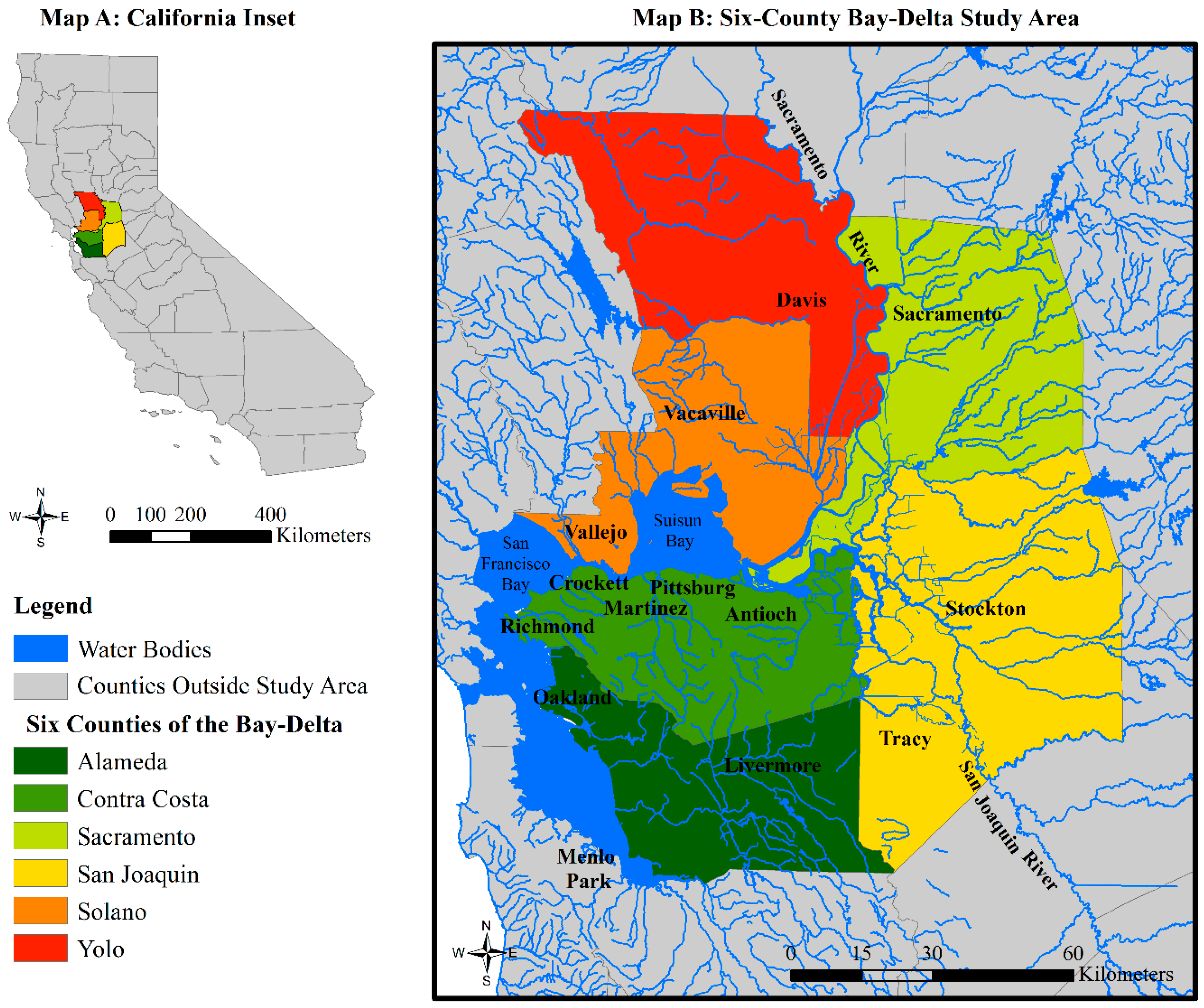
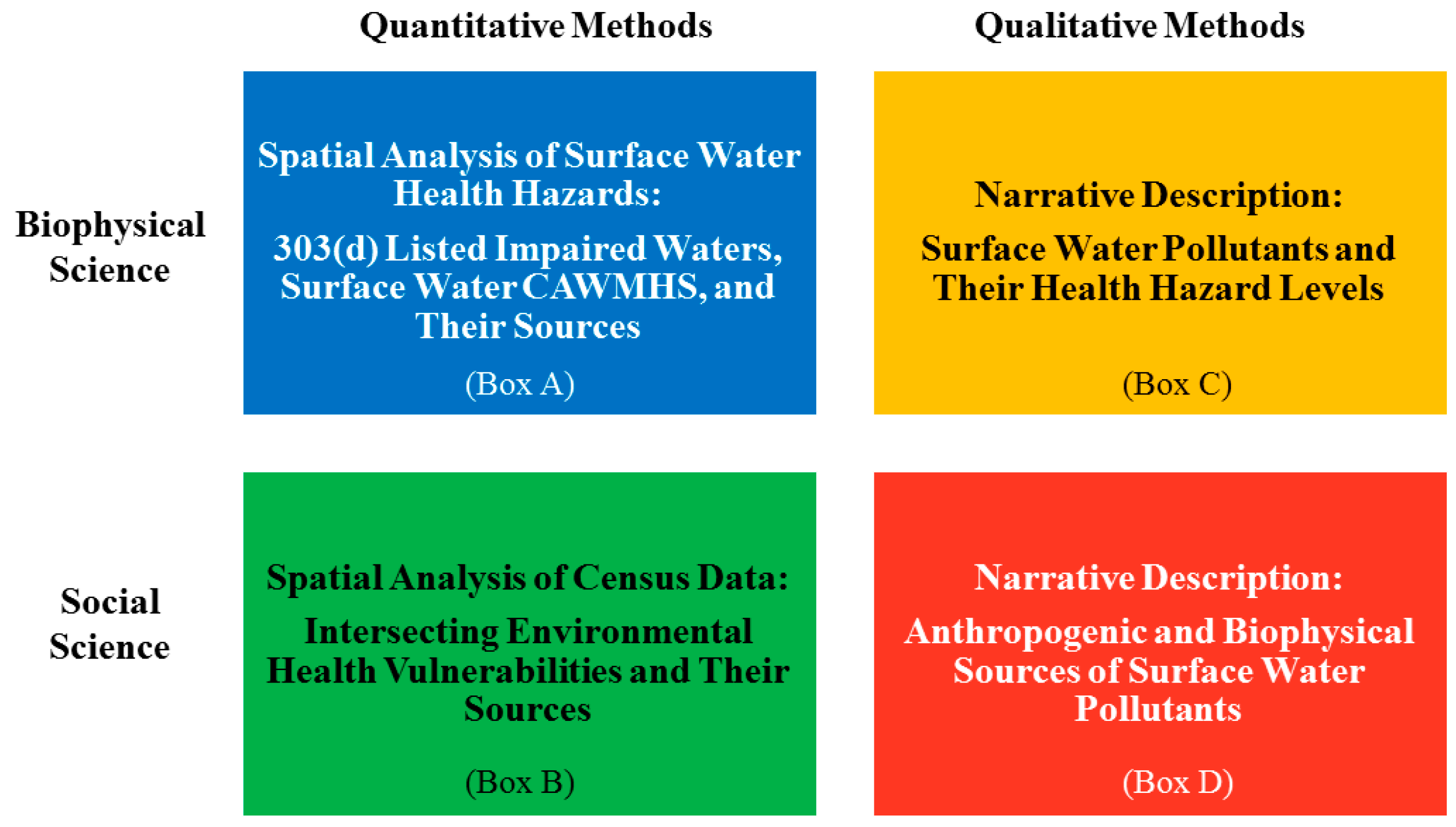
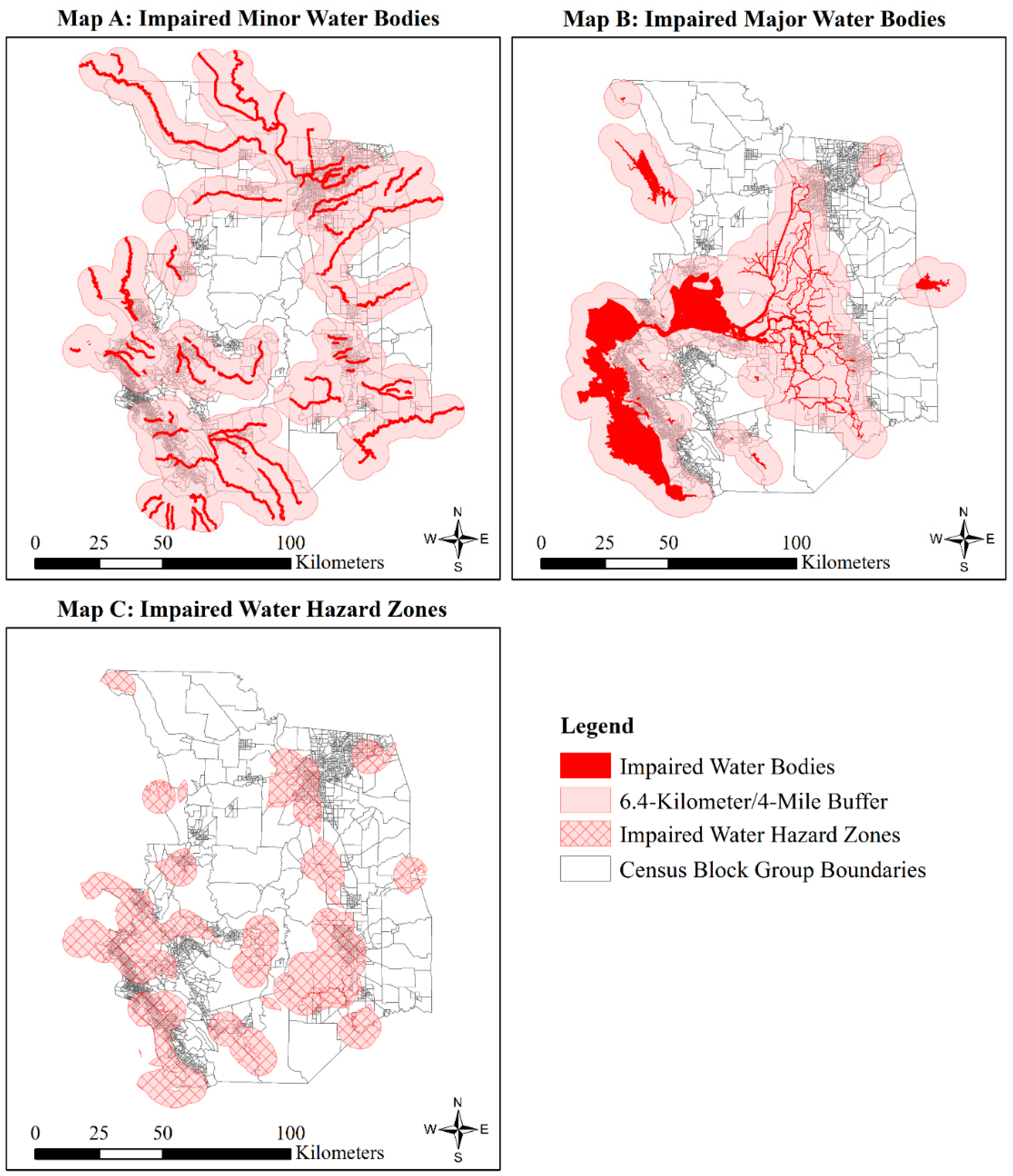
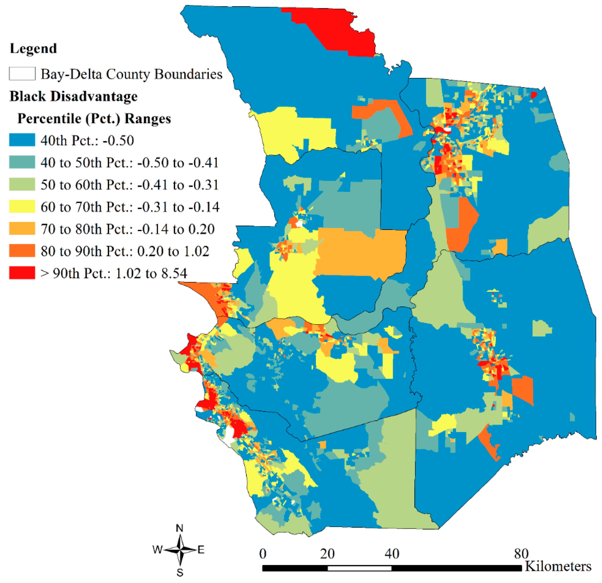
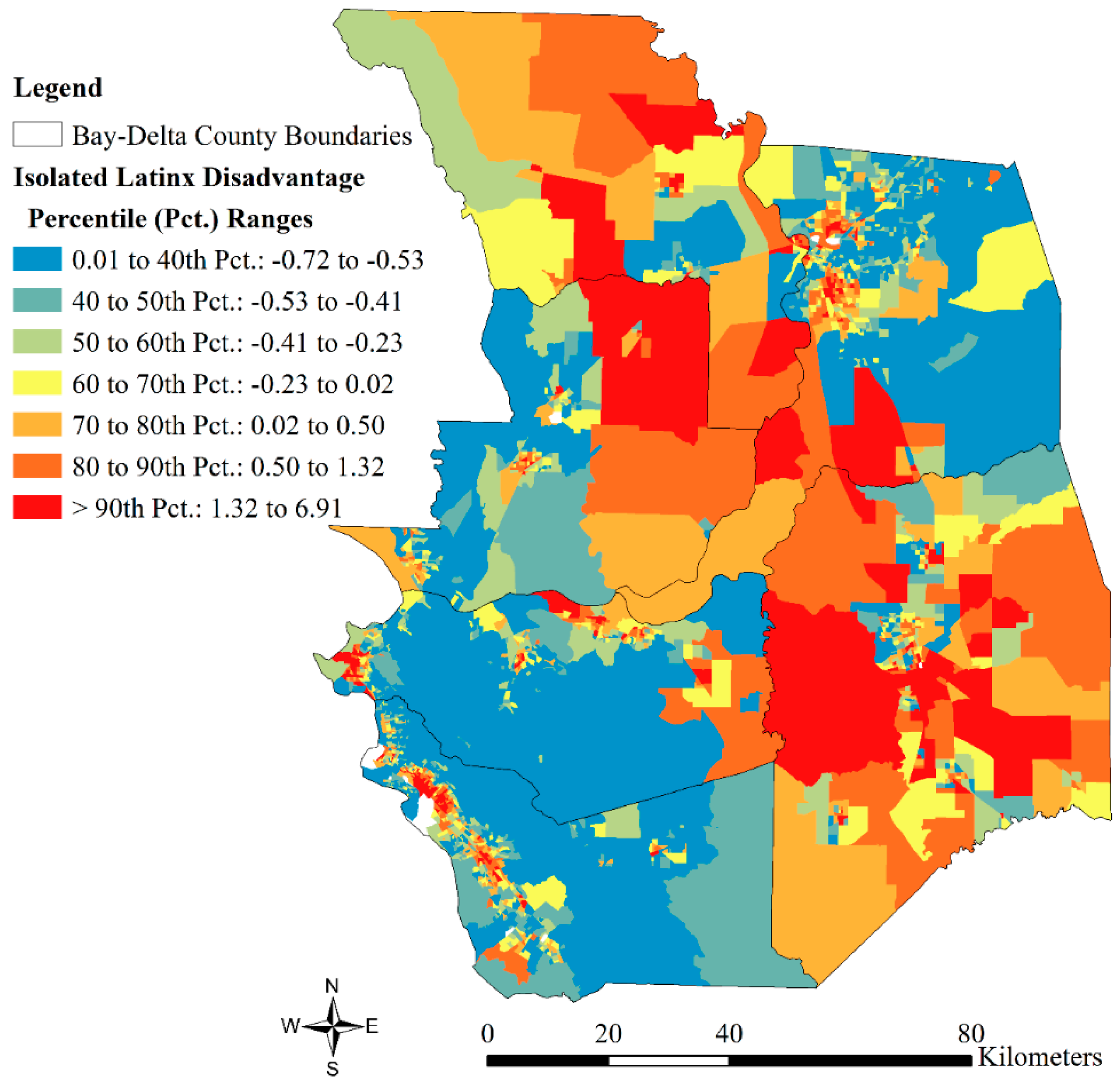
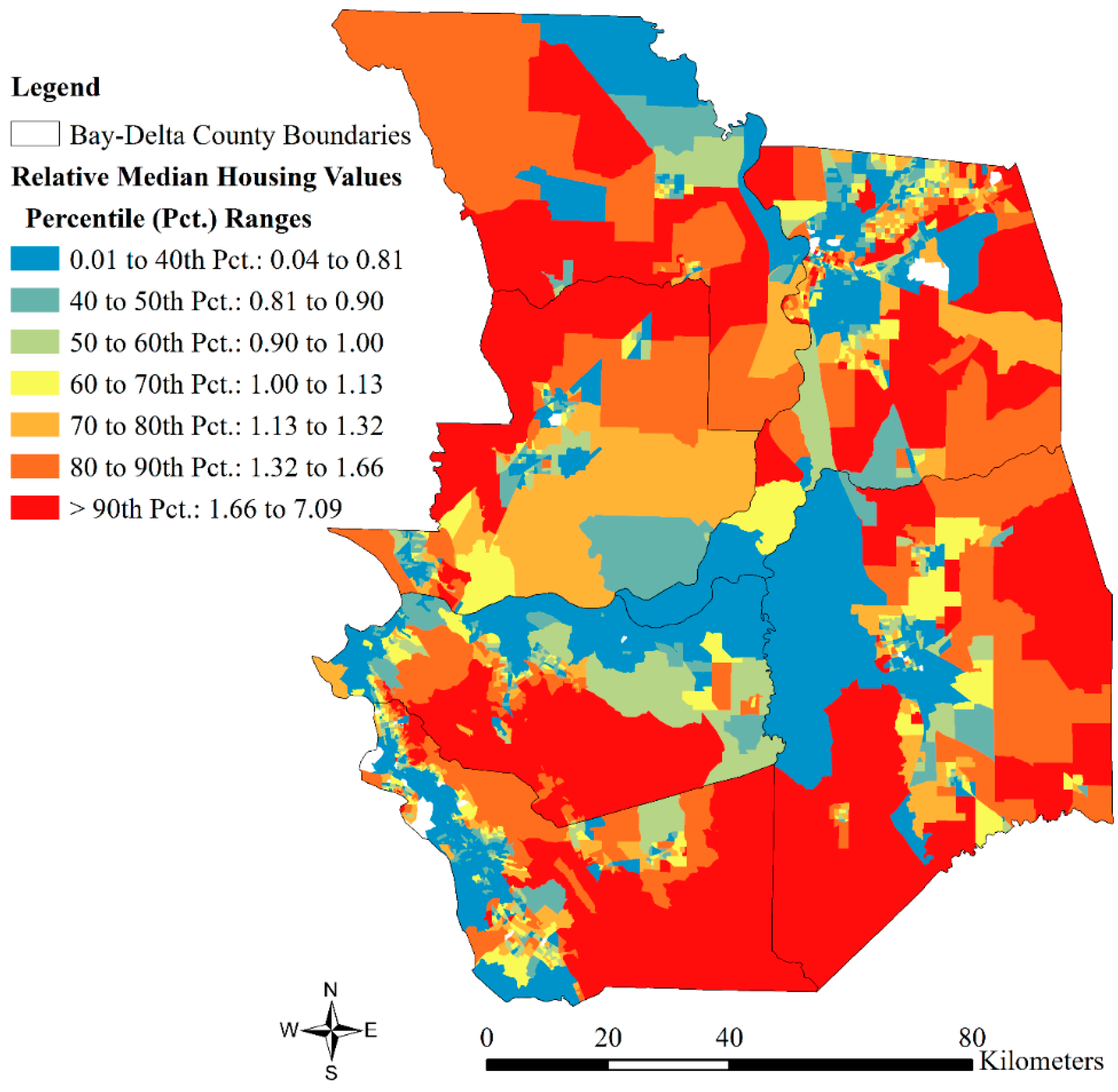
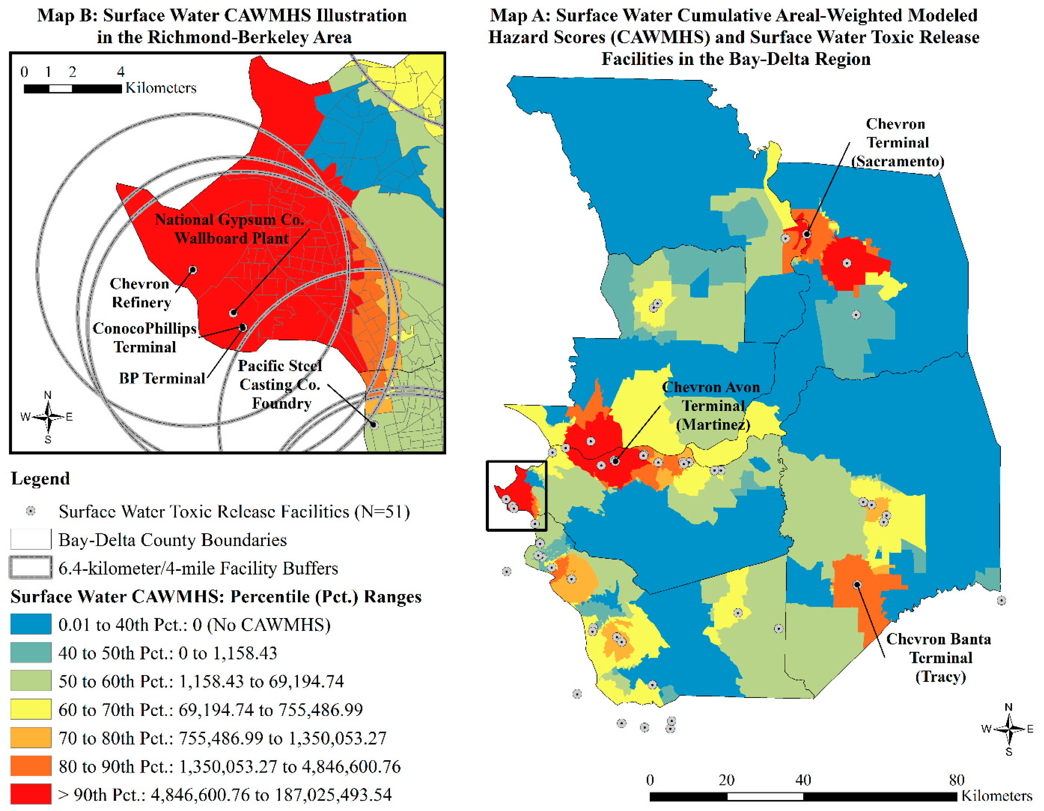
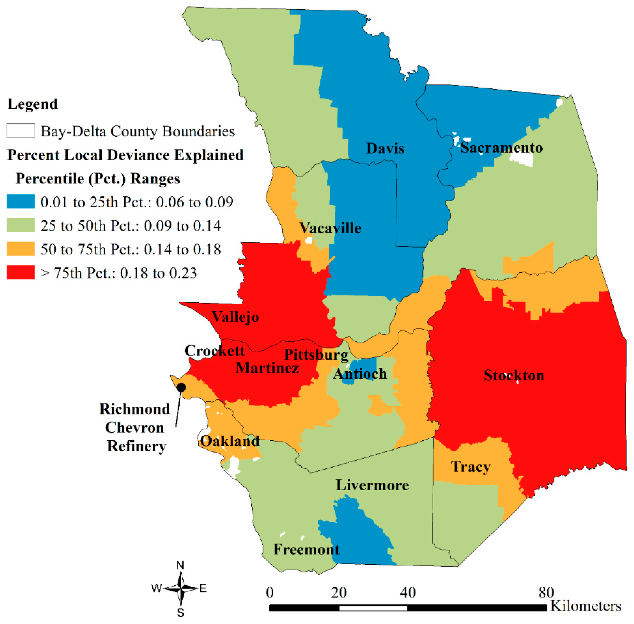
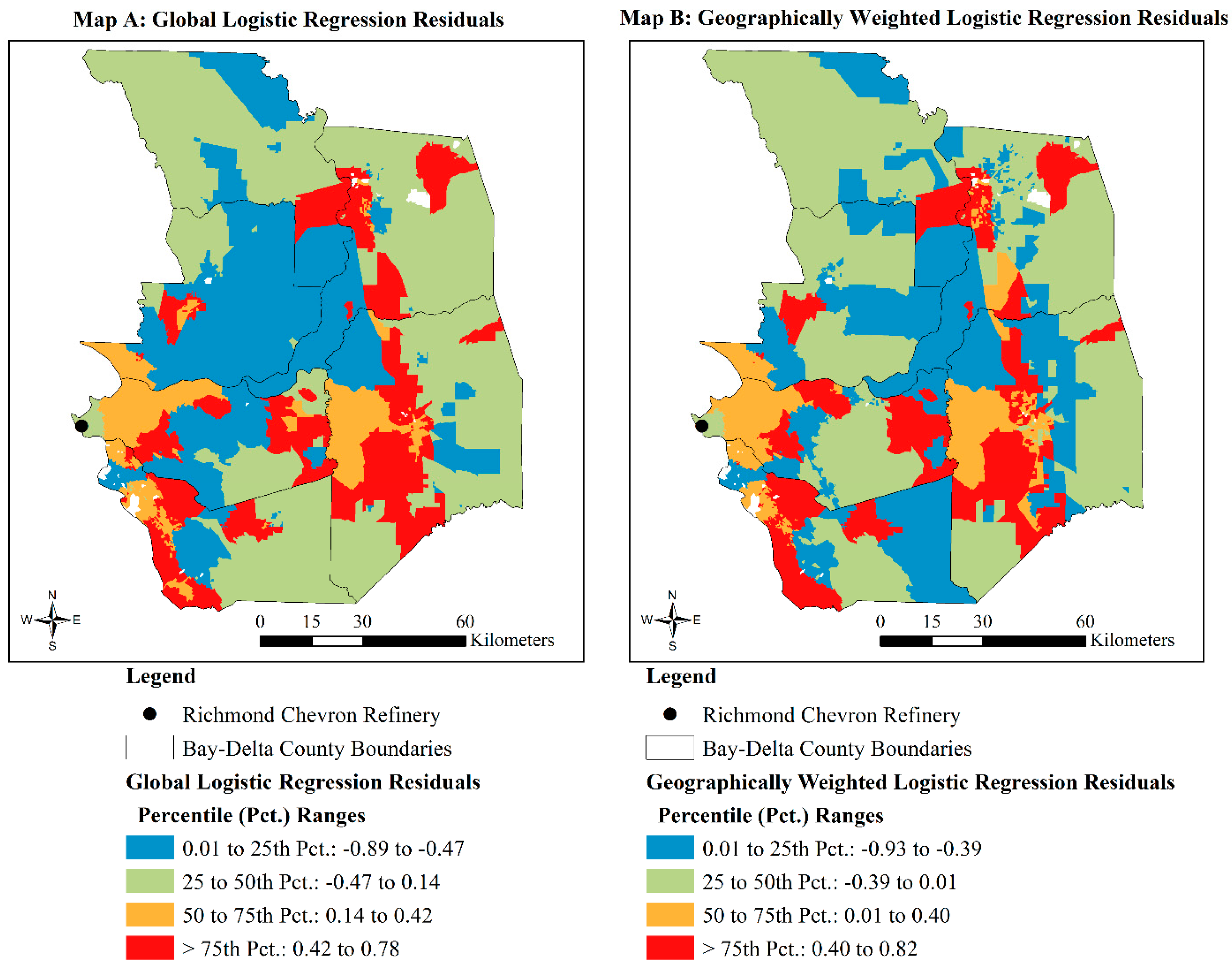
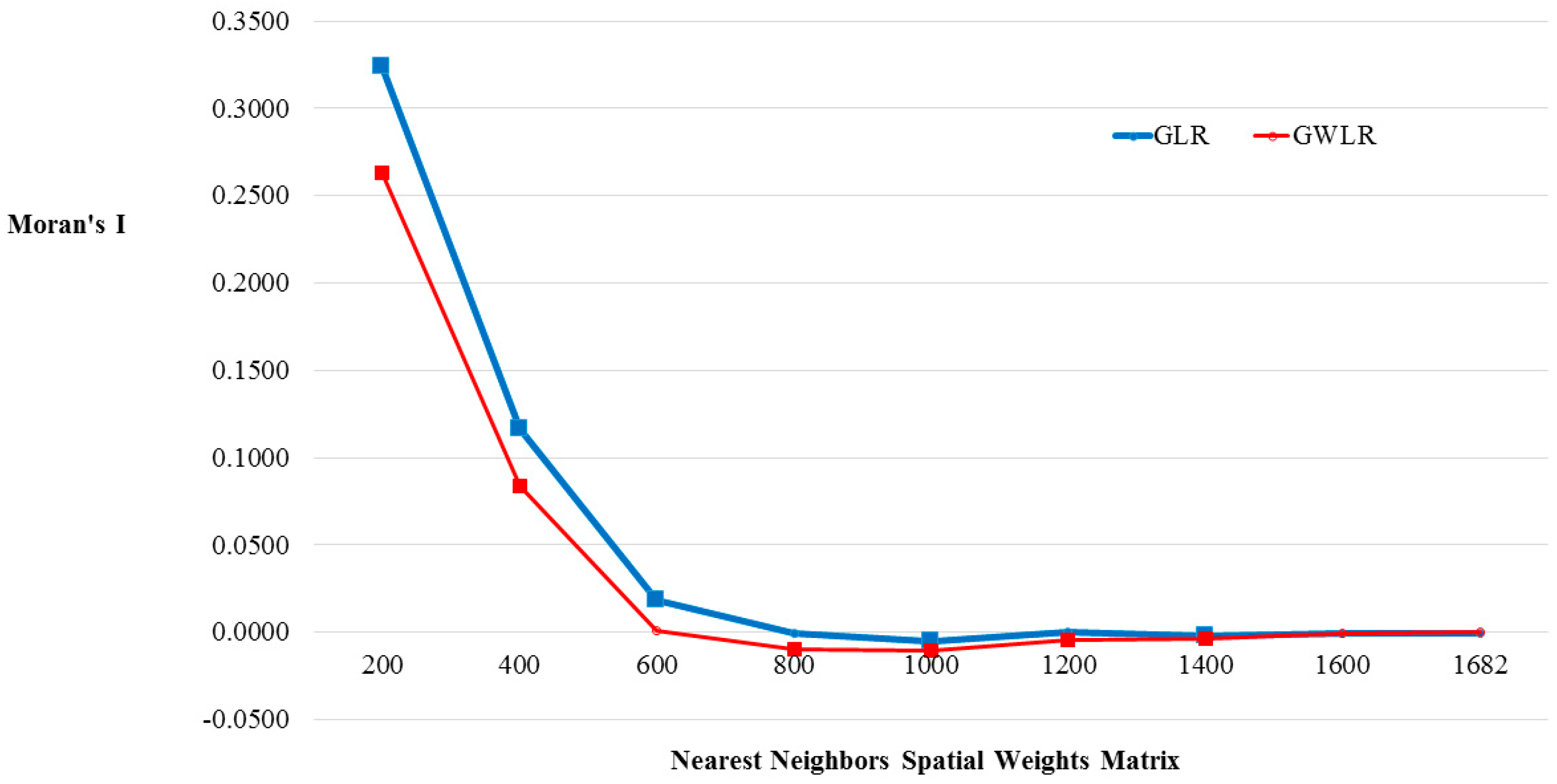
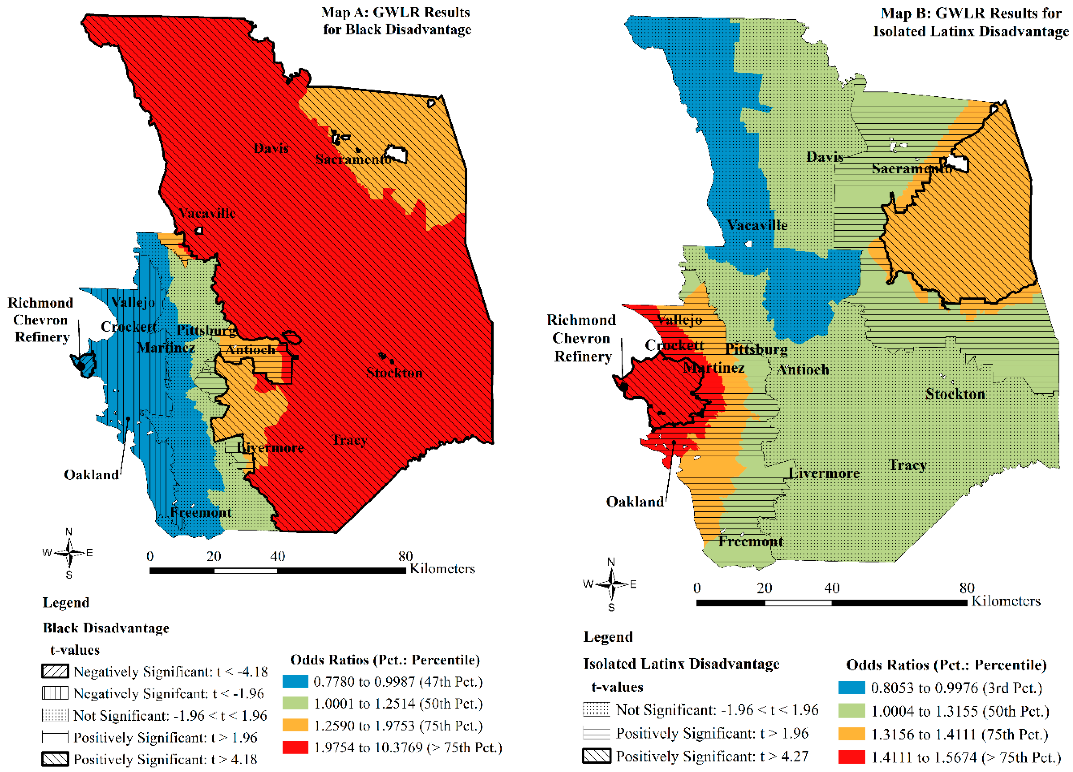
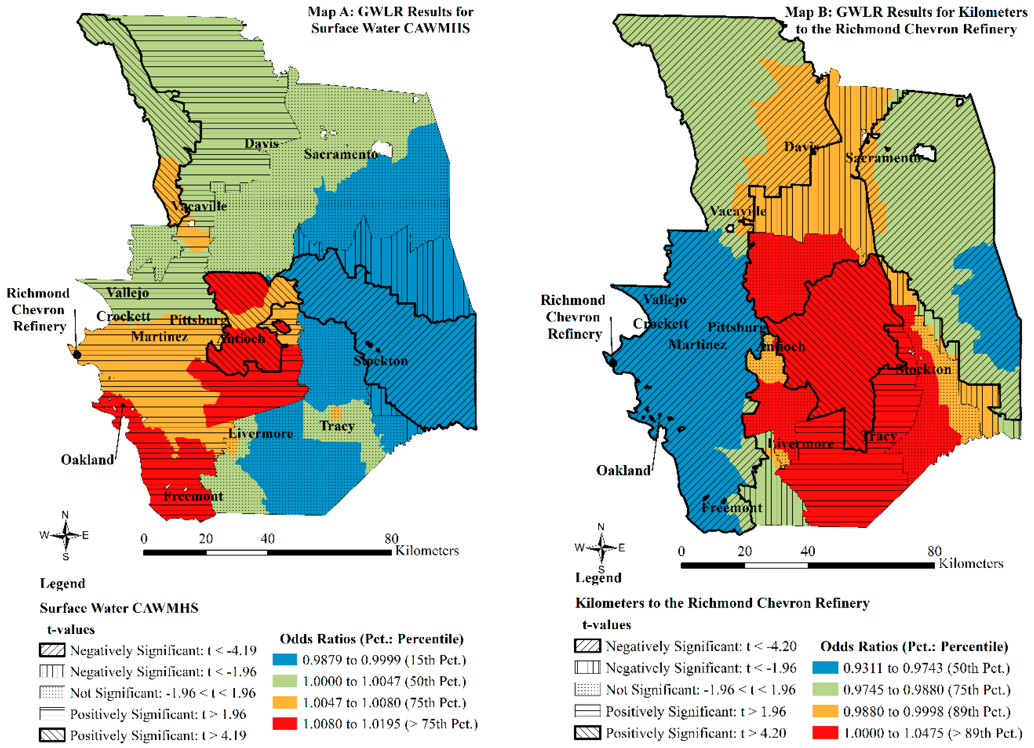
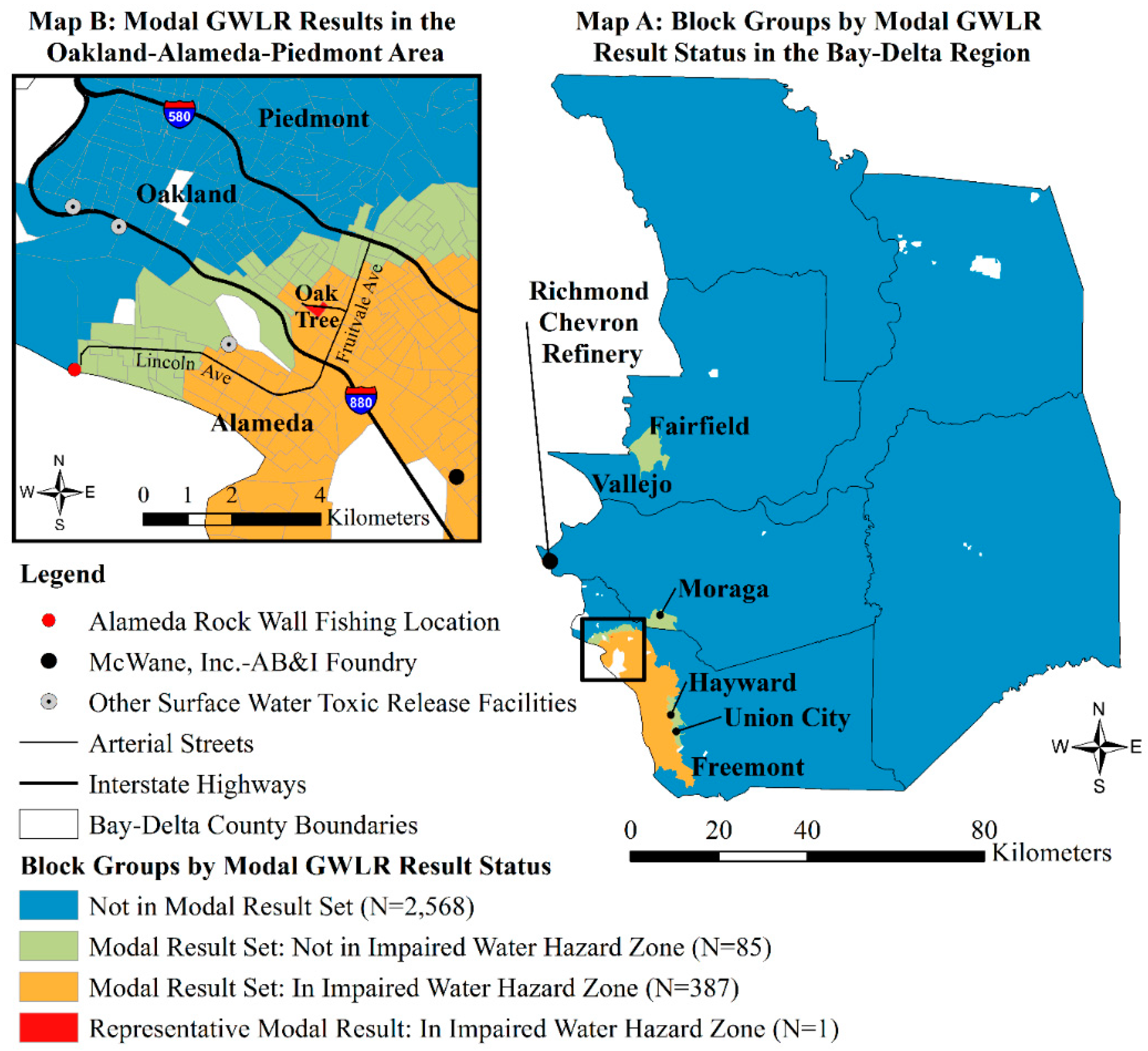
Table 1.
Principal component analysis results for intersecting population vulnerability factor variables [3].
Table 1.
Principal component analysis results for intersecting population vulnerability factor variables [3].
| Variables | Factor Loadings | |
|---|---|---|
| Black Disadvantage | Isolated Latinx Disadvantage | |
| Percent racial group: | ||
| Poor | 0.951 | 0.882 |
| No H.S. diploma | 0.951 | 0.946 |
| Percent linguistically isolated households: | ||
| Spanish speaking | 0.922 | |
| Cronbach’s alpha | 0.892 | 0.862 |
| Eigenevalue | 1.809 | 2.522 |
| % of total variance explained | 90.458 | 84.082 |
| N | 3064 | 3061 |
Table 2.
Surface water impairments by source category and frequency in the Bay-Delta, 2006.
| Source Category | Impairments | Proposed/U.S. EPA-Approved Completion Date | N Unique Pollutants 1 | ||
|---|---|---|---|---|---|
| N | % TMDL Required | N | Mean | ||
| Agriculture | 107 | 83.2 | 38 | 2013.6 | 22 |
| Urban runoff | 92 | 63 | 21 | 2015.3 | 16 |
| Unknown sources | 87 | 88.5 | 44 | 2011.7 | 33 |
| Unspecified NPS 2 | 63 | 100 | 62 | 2012.7 | 7 |
| Resource extraction | 42 | 95.2 | 18 | 2013.1 | 4 |
| Industrial wastewater | 36 | 100 | 34 | 2009.6 | 14 |
| Atmospheric deposition | 34 | 100 | 33 | 2013.6 | 3 |
| Municipal wastewater | 26 | 96.2 | 26 | 2011.3 | 13 |
| Miscellaneous | 19 | 100 | 19 | 2012.8 | 3 |
| Natural sources | 17 | 100 | 17 | 2011.5 | 2 |
| Unspecified point source | 9 | 100 | 9 | 2013.1 | 6 |
| Construction/Land Development | 8 | 100 | 0 | — | 3 |
| Hydromodification/Groundwater | 7 | 100 | 1 | 2010 | 6 |
| Non-boating recreational/tourism activity runoff | 7 | 100 | 1 | 2006 | 1 |
| Total | 554 | 88.3 | 323 | 2012.4 | 59 |
1 Most common pollutant was mercury, comprising 17.9% of all 554 impairments. 2 NPS, non-point-source.
Table 3.
Surface water toxic releases by industry classification and Risk-Screening Environmental Indicators (RSEI) [14] modeled hazard score, 2000−2006.
Table 3.
Surface water toxic releases by industry classification and Risk-Screening Environmental Indicators (RSEI) [14] modeled hazard score, 2000−2006.
| Two-Digit Standard Industry Classification | N Facilities | RSEI [14] Modeled Hazard Score of Toxic Releases | Most Hazardous Organization—City (Percent (%) Total Industry RSEI [14] Modeled Hazard Score) | |
|---|---|---|---|---|
| Total | Per facility | |||
| Petroleum Refining and Coal Products | 6 | 207,140,792.54 | 34,523,465.42 | Chevron Co. Refinery— Richmond (89.53%) |
| Transportation Equipment | 3 | 26,703,872.31 | 8,901,290.77 | John Boyd Enterprises/JB Radiator Specialties, Inc.—Sacramento (96.79%) |
| Wholesale Trade—Nondurable Goods | 6 | 17,653,062.30 | 2,942,177.05 | Chevron Co. Avon Terminal—Martinez (38.97%) |
| Primary Metal Industries | 5 | 3,043,414.14 | 608,682.83 | McWane, Inc./AB&I Foundry—Oakland (44.36%) |
| Rubber and Miscellaneous Plastics Products | 1 | 2,213,128.40 | 2,213,128.40 | Tyco Electronics Corp.— Menlo Park (100.00%) |
| Chemicals and Allied Products | 9 | 1,293,418.39 | 143,713.15 | Criterion Catalysts & Technologies, L.P.—Pittsburg (86.76%) |
| Electric, Gas, and Sanitary Services | 6 | 372,455.30 | 62,075.88 | Air Products & Chemicals, Inc./Stockton Cogen CO.— Stockton (77.60%) |
| National Security and International Affairs | 2 | 255,605.10 | 127,802.55 | U.S. Dept. of Energy National Laboratory—Livermore (99.29%) |
| Food and Kindred Products | 2 | 199,093.23 | 99,546.62 | C&H Sugar CO.—Crockett (99.99%) |
| Fabricated Metal Products | 4 | 76,673.00 | 19,168.25 | Shaw Group Inc. / Shaw Pipe Shields Inc.—Vacaville (93.91%) |
| Paper and Allied Products | 1 | 47,097.95 | 47,097.95 | Gaylord Container Corp.— Antioch (100.00%) |
| Electronic and Other Electric Equipment | 4 | 44,967.00 | 11,241.75 | Viktron California—Stockton (73.39%) |
| Engineering & Management Services | 1 | 36,000.00 | 36,000.00 | U.S. Dept. of Energy Lawrence Livermore National Laboratory Experimental Test Site (S300)— Tracy (100.00%) |
| Stone, Clay, and Glass Products | 1 | 5400.00 | 5400.00 | National Gypsum Co.— Richmond (100.00%) |
| Totals | 51 | 259,084,979.66 | 5,080,097.64 | Chevron Co. Refinery— Richmond (71.58%) |
Table 4.
Surface water toxic release facility ranked by RSEI [14] modeled hazard score for mercury releases and total releases, 2000–2006.
Table 4.
Surface water toxic release facility ranked by RSEI [14] modeled hazard score for mercury releases and total releases, 2000–2006.
| Facilities by RSEI [14] Modeled Hazard Score Rank for Mercury Releases (City) | Mercury Releases | All Surface Water Toxic Releases | Percent of Overall Modeled Hazard Score Associated with Mercury Releases | ||
|---|---|---|---|---|---|
| Pounds | RSEI [14] Modeled Hazard Score | Overall Hazard Rank | RSEI [14] Modeled Hazard Score | ||
| 1. Chevron oil refinery (Richmond) | 3.0000 | 30,000.00 | 1 | 185,456,128.24 | 0.0162 |
| 2. FPL Energy/POSDEF Power electric power facility (Stockton) | 0.6779 | 6779.00 | 22 | 49,298.00 | 13.7511 |
| 3. Valero Energy oil refinery (Benicia) | 0.2000 | 2000.00 | 3 | 19,435,900.20 | 0.0103 |
| 4. Tesoro oil refinery (Martinez) | 1.0000 | 1000.00 | 8 | 1,973,689.00 | 0.0507 |
| 5. AERC recycling center (Hayward) | 0.0028 | 28.02 | 46 | 28.02 | 100.0000 |
| 6. Air Products & Chemicals/Stockton CoGen coal-fired power station (Stockton) | 0.0021 | 20.70 | 16 | 289,012.08 | 0.0072 |
| 7. McWane Inc./AB&I foundry (Oakland) | 0.0004 | 3.77 | 10 | 1,350,003.77 | 0.0003 |
| 8. Shell oil refinery (Martinez) | 1.3000 | 0.00 | 23 | 48,016.00 | 0.0000 |
| 9. ConocoPhillips oil refinery (Rodeo) | 1.1300 | 0.00 | 18 | 227,009.60 | 0.0000 |
Table 5.
Comparison of block group means by 50 percent areal containment within a 2006, 303(d), impaired water hazard zone.
Table 5.
Comparison of block group means by 50 percent areal containment within a 2006, 303(d), impaired water hazard zone.
| Variables | Block Group 50 Percent Areal Containment in Impaired Water Hazard Zone | |
|---|---|---|
| Yes | No | |
| Population vulnerability | ||
| Black disadvantage, 2000 | 0.14 | −0.16 |
| N | 1633 | 1431 |
| Isolated Latinx disadvantage, 2000 | 0.14 | −0.16 |
| N | 1631 | 1430 |
| Uneven development | ||
| Relative median housing value, 2000 | 0.95 | 1.08 |
| N | 1617 | 1424 |
| Contemporary industrial pollution sources | ||
| Kilometers to Richmond Chevron refinery | 54.26 | 74.76 |
| Surface water CAWMHS, 2000–2006 (100,000 s) | 105.45 | 17.04 |
| N | 1637 | 1436 |
Table 6.
Descriptive statistics for variables used in the global logistic regression (GLR) and geographically weighted logistic regression (GWLR) analyses of block group 50 percent areal containment within a 2006, 303(d), impaired water hazard zone (N = 3041).
Table 6.
Descriptive statistics for variables used in the global logistic regression (GLR) and geographically weighted logistic regression (GWLR) analyses of block group 50 percent areal containment within a 2006, 303(d), impaired water hazard zone (N = 3041).
| Variables | Mean | SD | Min. | Max. | Moran’s I 1 |
|---|---|---|---|---|---|
| Population vulnerability | |||||
| Black disadvantage, 2000 | 0.00 | 0.99 | −0.50 | 8.54 | 0.022 *** |
| Isolated Latinx disadvantage, 2000 | 0.00 | 1.00 | −0.72 | 6.91 | 0.003 *** |
| Uneven development | |||||
| Relative median housing value, 2000 | 1.01 | 0.52 | 0.04 | 7.09 | −0.001 *** |
| Contemporary industrial pollution sources | |||||
| Kilometers to Richmond Chevron Refinery | 63.83 | 39.96 | 1.26 | 139.20 | 0.636 *** |
| Surface water CAWMHS, 2000–2006 (100,000 s) | 64.61 | 291.37 | 0.00 | 1870.25 | 0.014 *** |
1 The spatial autocorrelation analysis of the independent variables used a 1682-nearest neighbor spatial weights matrix and 9999 permutations; *** Pseudo p < 0.001 (two-tailed test).
Table 7.
GLR results for block group 50 percent areal containment within a 2006, 303(d), impaired water hazard zone on population vulnerability, uneven development, and contemporary industrial pollution sources (N = 3401 block groups).
Table 7.
GLR results for block group 50 percent areal containment within a 2006, 303(d), impaired water hazard zone on population vulnerability, uneven development, and contemporary industrial pollution sources (N = 3401 block groups).
| Variables | B | S.E. | OR | 95% C.I. for OR |
|---|---|---|---|---|
| Population vulnerability | ||||
| Black disadvantage, 2000 | 0.106 * | 0.049 | 1.111 | 1.009−1.224 |
| Isolated Latinx disadvantage, 2000 | 0.309 *** | 0.047 | 1.362 | 1.242−1.494 |
| Uneven development | ||||
| Relative median housing value, 2000 | −0.127 | 0.084 | 0.881 | 0.747−1.038 |
| Contemporary industrial pollution sources | ||||
| Kilometers to Richmond Chevron refinery | −0.013 *** | 0.001 | 0.987 | 0.985−0.989 |
| Surface water CAWMHS, 2000–2006 (100,000 s) | 0.002 *** | 0.001 | 1.002 | 1.001−1.003 |
| Intercept | 1.058 *** | 0.117 | 2.881 | |
| Model diagnostics | ||||
| −2 log likelihood | 3845.220 | |||
| Model chi-square | 358.244 *** | |||
| Degrees of freedom | 5 | |||
| Nagerlkerke R2 | 0.148 | |||
* p < 0.05; *** p < 0.001 (two-tailed test).
Table 8.
Comparison of model goodness-of-fit statistics.
| Model | Deviance | df | Deviance/df | Percent Deviance Explained | AIC | Number of Parameters |
|---|---|---|---|---|---|---|
| GLR | 3845.22 | 3035 | 1.27 | 0.085 | 3857.22 | 6 |
| GWLR | 3475.44 | 3019 | 1.15 | 0.173 | 3513.31 | 18.94 |
GLR, global logistic regression; GWLR, geographically weighted logistic regression; AIC, Akaike information criterion; df, degrees of freedom.
Table 9.
Summary statistics for the GWLR results for block group 50 percent areal containment within a 2006, 303(d), impaired water hazard zone on population vulnerability, uneven development, and contemporary industrial pollution source factors (N = 3401 block groups).
Table 9.
Summary statistics for the GWLR results for block group 50 percent areal containment within a 2006, 303(d), impaired water hazard zone on population vulnerability, uneven development, and contemporary industrial pollution source factors (N = 3401 block groups).
| Variables | Model Coefficients | Percent of Block Groups by Significance Level of t-Value | |||||||
|---|---|---|---|---|---|---|---|---|---|
| Min. | Median | Max. | FDR t-Value | t < −FDR t-Value | t < −1.96 | −1.96 < t < 1.96 | t > 1.96 | t > +FDR t-Value | |
| Population vulnerability | |||||||||
| Black disadvantage, 2000 | −0.251 | 0.224 | 2.340 | 4.18 | 1.41 | 34.30 | 13.84 | 5.23 | 45.22 |
| Isolated Latinx disadvantage, 2000 | −0.217 | 0.274 | 0.449 | 4.27 | 0.00 | 0.00 | 22.10 | 63.56 | 14.34 |
| Uneven development | |||||||||
| Relative median housing value, 2000 | −0.956 | −0.193 | 0.407 | 4.25 | 1.41 | 34.92 | 36.57 | 27.10 | 0.00 |
| Contemporary industrial pollution sources | |||||||||
| Kilometers to Richmond Chevron Refinery | −0.071 | −0.026 | 0.046 | 4.20 | 81.52 | 4.83 | 8.42 | 3.85 | 1.38 |
| Surface water CAWMHS, 2000–2006 (100,000 s) | −0.012 | 0.005 | 0.019 | 4.19 | 10.29 | 1.64 | 30.29 | 55.44 | 2.33 |
| Intercept | −2.932 | 1.793 | 4.034 | 4.24 | 1.32 | 0.39 | 17.43 | 20.29 | 60.57 |
FDR, false discovery rate.
Table 10.
Representative block group from modal GWLR results for block group 50 percent areal containment within a 2006, 303(d), impaired water hazard zone on population vulnerability, uneven development, and contemporary industrial pollution source factors.
Table 10.
Representative block group from modal GWLR results for block group 50 percent areal containment within a 2006, 303(d), impaired water hazard zone on population vulnerability, uneven development, and contemporary industrial pollution source factors.
| Variables | Representative Block Group: Oak Tree Neighborhood in Oakland (ID: 060014062013) | |||||
|---|---|---|---|---|---|---|
| Value | GWLR Results | |||||
| B | S.E. | t-Value | Sig. | OR | ||
| Population vulnerability | ||||||
| Black disadvantage, 2000 | −0.161 | −0.183 | 0.056 | −3.288 | 0.001 | 0.833 |
| Isolated Latinx disadvantage, 2000 | 5.458 | 0.371 | 0.093 | 3.985 | 6.9 × 10⁻⁵ | 1.450 |
| Uneven development | ||||||
| Relative median housing value, 2000 | 0.573 | −0.263 | 0.126 | −2.091 | 0.037 | 0.769 |
| Contemporary industrial pollution sources | ||||||
| Kilometers to Richmond Chevron Refinery | 21.950 | −0.042 | 0.005 | −9.268 | 3.5 × 10⁻²⁰ | 0.958 |
| Surface water CAWMHS, 2000–2006 (100,000 s) | 1350.166 | 0.008 | 0.002 | 3.297 | 9.9 × 10⁻⁴ | 1.008 |
| Intercept | 2.041 | 0.216 | 9.459 | 6.0 × 10⁻²¹ | 7.695 | |
| Model diagnostics | ||||||
| Percent local deviance explained | 0.150 | |||||
© 2018 by the author. Licensee MDPI, Basel, Switzerland. This article is an open access article distributed under the terms and conditions of the Creative Commons Attribution (CC BY) license (http://creativecommons.org/licenses/by/4.0/).
Share and Cite
MDPI and ACS Style
Liévanos, R.S. Impaired Water Hazard Zones: Mapping Intersecting Environmental Health Vulnerabilities and Polluter Disproportionality. ISPRS Int. J. Geo-Inf. 2018, 7, 433. https://0-doi-org.brum.beds.ac.uk/10.3390/ijgi7110433
AMA Style
Liévanos RS. Impaired Water Hazard Zones: Mapping Intersecting Environmental Health Vulnerabilities and Polluter Disproportionality. ISPRS International Journal of Geo-Information. 2018; 7(11):433. https://0-doi-org.brum.beds.ac.uk/10.3390/ijgi7110433
Chicago/Turabian StyleLiévanos, Raoul S. 2018. "Impaired Water Hazard Zones: Mapping Intersecting Environmental Health Vulnerabilities and Polluter Disproportionality" ISPRS International Journal of Geo-Information 7, no. 11: 433. https://0-doi-org.brum.beds.ac.uk/10.3390/ijgi7110433
Note that from the first issue of 2016, this journal uses article numbers instead of page numbers. See further details here.