Spatial Distribution Estimates of the Urban Population Using DSM and DEM Data in China


1
Key Laboratory of Environmental Change and Natural Disaster of Ministry of Education, Faculty of Geographical Science, Beijing Normal University, Beijing 100875, China
2
State Key Laboratory of Earth Surface Processes and Resource Ecology, Beijing Normal University, Beijing 100875, China
3
Academy of Disaster Reduction and Emergency Management, Ministry of Civil Affairs and Ministry of Education, Beijing 100875, China
4
Faculty of Information Engineering, China University of Geosciences, Wuhan, 430074, China
*
Authors to whom correspondence should be addressed.
ISPRS Int. J. Geo-Inf. 2018, 7(11), 435; https://0-doi-org.brum.beds.ac.uk/10.3390/ijgi7110435
Submission received: 5 September 2018
/
Revised: 16 October 2018
/
Accepted: 4 November 2018
/
Published: 7 November 2018
Abstract
:Spatial distribution and population density are important parameters in studies on urban development, resource allocation, emergency management, and risk analysis. High-resolution height data can be used to estimate the total or spatial pattern of the urban population for small study areas, e.g., the downtown area of a city or a community. However, there has been no case of population estimation for large areas. This paper tries to estimate the urban population of prefectural cities in China using building height data. Building height in urban population settlement (Mdiffs) was first extracted using the digital surface model (DSM), digital elevation model (DEM), and land use data. Then, the relationships between the census-based urban population density (CPD) and the Mdiffs density (MDD) for different regions were regressed. Using these results, the urban population for prefectural cities of China was finally estimated. The results showed that a good linear correlation was found between Mdiffs and the census data in each type of region, as all the adjusted R2 values were above 0.9 and all the models passed the significance test (95% confidence level). The ratio of the estimated population to the census population (PER) was between 0.7 and 1.3 for 76% of the cities in China. This is the first attempt to estimate the urban population using building height data for prefectural cities in China. This method produced reasonable results and can be effectively used for spatial distribution estimates of the urban population in large scale areas.

1. Introduction
The spatial pattern of regional populations is closely related to the geographical, societal, and economic environments, as well as to natural resources. Understanding the population size, density, and spatial distribution is beneficial for urban planning, resource allocation, and disaster risk management [1]. Census population data, geographic information system (GIS), and remote sensing data, and social media data are currently major sources for demographic studies.
Census data are relatively accurate; however, they are labor intensive and time consuming to obtain and update. They are based on the administrative unit and have low spatial resolution, and do not reflect dynamic changes in population in a timely manner [2,3]. These limitations make it necessary to develop alternative techniques and methods to improve the accuracy, time resolution, and spatial resolution.
Currently, mobile phone data and social media data, such as mobile call data [4,5,6], WiFi data [7,8], and social networking service software data [9,10,11], which have short acquisition periods and high timeliness, are popular methods to estimate population density, distribution, and mobility. Deville et al. used mobile phone data to estimate the urban population density of Portugal, and the accuracy of the estimation results was increased by comparing the results with census data at an administrative division level and remote sensing data at a 100 m×100 m grid scale [4]. However, the users of mobile phones and social media service software do not cover the whole country [12], so that the estimated total population might be low if only big data sources are used. Due to privacy, the aforementioned data may be difficult to obtain and thus cannot be widely used, which represents another difficulty when estimating population mobility.
Remote sensing has become an important method of performing population estimates in the past four decades [13] and many methods have been reported in the GIS and remote sensing literature. Depending on the intended goal and the required information, these methods can be grouped into two categories: Areal interpolation and statistical modeling [14]. The former is primarily designed for zone transformation that involves transforming data from one set of spatial units to another [13,15]. How to define source zones and target zones, the degree of generalization in the interpolation process, and the characteristics of the partitioned surface influence the quality of the interpolation estimates [16]. Areal interpolation methods can be further separated into two categories depending on whether ancillary information is used. The statistical modeling approach is more interested in inferring the relationship between the population and other variables, such as urban areas, land use, dwelling units, image pixel characteristics, and other physical or socioeconomic characteristics, in order to estimate the total population of an area [17,18]. The quality of the statistical modeling approach depends on how to select the related variables and statistical model.
Landsat satellite data, land use/cover data, nighttime light data, digital elevation model (DEM) data, and some high-resolution remote sensing images are commonly utilized to estimate population. With the development of light detection and ranging (LiDAR) technology, the height data of a building can be obtained and applied to gradually estimate regional population. Some research on population estimation using height data and the statistical modeling approach has been published. In 2010, Lu et al. [19] examined the utility of QuickBird imagery and LiDAR data for estimating population at the census-block level using two approaches: Area-based and volume-based. Residential building footprints were first delineated from the remote-sensing data using classification algorithms. Regression analysis was used to model the relationship between the population and the area or volume of the delineated residential buildings. Both approaches were successful in terms of estimating the population with high accuracy, finding that the root mean square error (RMSR) was equal to 10–30 people. The number, area and volume of buildings for residential and commercial parcels were first calculated using the digital surface model (DSM) and LiDAR-data-based DEM data, and then were regressed using the census population. The result showed an underestimation of the population density due to the lack of high-resolution image data [20]. In 2013, Alahmadi et al. [21] classified their study area using Enhanced Thematic Mapper (ETM+) data using the iterative self-organizing data analysis technique (ISODATA) and support vector machine (SVM) algorithms in order to extract building area land cover type; then height data was used to refine the building area, which was regressed using the density of the dwelling units for the population estimation. The result showed that the SVM classification algorithm and building area refined by height data improved the accuracy. Later, in 2016, they improved their previous work using height data, and the results showed higher accuracy [22]. Xie et al. [23] extracted the height, area, and volume of buildings using a morphological building detection algorithm; these variables were then utilized to classify and collect residential buildings; finally, the height, area, and volume of residential buildings were regressed using the population. The results showed that the RMSE and mean absolute relative error (MARE) of the population estimation were 13 and 33.52%, respectively.
It can be concluded that high-resolution height data can be well used to estimate the total or spatial pattern of the urban population for small study areas, e.g., the downtown area of a city or a community. However, there is a lack of evidence as to whether height data can be used to estimate the total urban population of large areas. In this paper, height data was used to estimate the urban population of prefectural cities in China. The building height in urban areas was first obtained according to the DSM and DEM datasets. Next, three algorithms were used to classify the whole search area, and then regression models between the census population density and total building height were built and analyzed for the prefectural cities. By comparing the regression results and through comprehensive analysis, an optimum classification algorithm was developed. Subsequently, the population of China was estimated using the regression models from the optimum classification algorithm, and the results were finally compared with the census population.
2. Data and Method
2.1. Data
The data used in this paper mainly include DSM, DEM, land use data, census data, and basic geographic information data. Details are shown in Table 1.
The DSM captures natural and built features on the earth’s surface. Only 30 m resolution data is available, thus it needed to be resampled to 1 km. DEM is a 3D, computer-generated, graphical representation of a terrain’s surface, and only represents the bare-earth height information without any further definition about the surface. Land use data shows the type of a certain district. The land use data used in this paper includes the natural landscape, human activity areas, and unutilized land. The human activity areas include urban land, suburban settlements, and construction land. Urban land refers to large, medium, and small cities, and some built-up areas which rank above counties and towns. The total number of land use types is 26, each of which is recorded by a code. Urban areas are coded as 51. The census population data used in this paper refer to the permanent resident population from the sixth national population census of China. All the data are projected with equal-area Albers.
2.2. Method
The technical flow of estimating the population using the proposed method in this study is shown in Figure 1. The method includes the following three steps:
Step 1: Calculation of Building Height and Calibration of Mdiffs
The DSM data values represent the elevation of the surface including built up features, and the DEM data values represent the bare-earth elevation of the terrain, thus the average height (diffs) data can be calculated according to Equation (1).
The digital number (DN) value of the diffs data in urban areas was referred to as Mdiffs and was approximately equal to the average height of the buildings. Urban areas were defined by the urban land type in land use data where there was an urban population.
Outliers with very large and negative values were observed in the Mdiffs data. Outliers less than 0 were changed to 0 in theory. As for outliers with very large values, an accurate range could not be obtained. In order to ensure a relatively reasonable range, the 30 m resolution DSM and DEM data for some large urbanized cities may be helpful: The Mdiffs with 30m resolution was able to be obtained directly according to Equation (1) and the land use data. Then, the negative values were changed to 0. Next, the Mdiffs of these cities were resampled to 1 km resolution, and their maximum value was Dmax, which was the maximum value of the Mdiffs data with 1km resolution for all of China.
Step 2: Classifying the Study Area
In view of the large area and geographic regional diversity in China, the whole study area should be classified into different categories. In urban areas, a linear relationship between building height and population size was assumed if differences in land use were not considered. Population and Mdiffs were the feature variables of each prefectural region or prefectural city in China. Their ratio (Equation (2)) could reflect the average population density in the 3D space or the average vacancy rate of a city. It is advantageous to study result if cities with similar features can be divided into a class.
where CPD and MDD represent the urban population density from the census data (unit: People/km2) and the density of Mdiffs at the prefectural city level (unit: Meter/km2), respectively. The K value is reasonable as long as both the CPD and MDD are larger than zero.
The prefectural cities of China were then classified according to the K index and the classification code was recorded as k. Firstly, a box plot was graphed to describe the outliers and interquartile range. Then the k-medoids algorithm was applied to confirm the optimum clustering number (Cnum) and the clustering result. After that, the hierarchical clustering algorithm was also tried in R language to divide the Cnum categories. Finally, the results of the three methods were compared to obtain the optimum method for the population estimate.
Step 3: Urban Population Estimation
Based on the classification results of the different algorithms, the density of the census population (CPD), which was chosen as the dependent variable, was fitted with density of Mdiffs (MDD) using the linear regression model through the origin in each k class. This model was adopted because the population of a region should be zero if its MDD value is zero. Then the statistical information of the regression models based on the different classification results was compared and integrated to find the optimum classification algorithm whose regression coefficients were recorded as aki. The aki for all pixels in region k is assumed to be equivalent; thus, the gridded urban population in region k can be calculated according to Equation (3). Thus, the total urban population in China can be obtained by the summation of the estimated total urban population of the different regions.
where GEPki is the estimated population for each grid i in region k; aki is the coefficient; and DNki is the DN value of the Mdiffs data of grid i in region k.
3. Results and Discussion
3.1. Results
Beijing, Shanghai, Guangzhou are the most urbanized and developed cities in China. Therefore, they were selected to calibrate the outliers. The value of Dmax was set to 100 in this paper.
The K values of 344 cities were available (there are two cities where there was no Mdiffs). The box plot of the K index showed that the maximum, median and minimum values were 6178.840, 2214.419, and 267.656, respectively, and the upper and lower quartile values were 3338.423 and 1392.929, respectively. The value >6178.840 was an outlier. The result of k-medoid clustering was Cnum = 6; outliers and normal values were divided into two and four categories, respectively. The hierarchical clustering algorithm divides the outliers into three parts and the normal values into three parts. The classification results of the three algorithms were applied to fit the relationship of the urban census population density (CPD) and Mdiffs density (MDD).
Table 2 shows the classification and regression results. As for the normal values, the adjusted R2 of the box plot was higher than the k-medoids and hierarchical clustering; the standard deviation of the standard residual (SD of the std. residual) of the box plot was lower than that of the hierarchical clustering, but roughly similar to that of the k-medoids. As for outliers, the k-medoid was similar to the box plot no matter whether the fifth and sixth categories were merged. Hierarchical clustering is more sensitive to outliers, but the regression model was not significant for the fifth category, which might be caused by a lower sample number. Thus, the paper integrated the sixth category into the fifth category for hierarchical clustering, which highly improved the result for the outliers. Therefore, the box plot algorithm was outstanding for the normal value clustering while hierarchical clustering was excellent for the outliers clustering. Considering that the number of normal samples was larger than that of the outlier samples, the results of the outliers for hierarchical clustering were applied to replace the results of the outliers for the box plot. Based on two previous adjustments, an adjusted box plot algorithm (shown in Table 2) was built, which was an optimum algorithm: The clustering number was 6, which is optimum; adjusted R2 and SD of the std. residual for each category were better than the other results.
The paper selected the classification results of the adjusted box plot (Figure 2). The regression equations were available. Therefore, in Equation (3), a1i = 1118.123, a2i = 1777.533, a3i = 2684.094, a4i = 4586.383, a5i = 6641.906, and a6i = 8910.301.
Figure 3 shows the distribution of the estimated urban population (EP) and census urban population (CP) at the prefectural city level. The spatial pattern of the estimated population was the same as for the census population. Table 3 shows the statistical results of the number and percentage of the prefectural cities with different population sizes and density grades. As for the population size, the blue area with an urban population of less than 100,000 covered five cities; the cyan area with an urban population of 100,000–500,000 covered 36 cities; the green area with an urban population of 500,000–1 million covered 73 cities; the yellow area with an urban population of 1–2 million covered 112 cities; the orange area with an urban population of 2–5 million covered 94 cities; and the red area with an urban population larger than 5 million covered 24 cities. There is the largest difference between EP and CP in grade (2000, 5000] (orange color), while smallest difference in grade (1000, 2000] (yellow color). As for population density, the 13 cities with a population density larger than 1000 persons/km2 (red) were mainly distributed in the areas of Beijing–Tianjin, Shanghai, and Guangzhou–Shenzhen. The 84 cities with a population density smaller than 50 persons/km2 (blue) were mainly distributed in western China. The cities with a high population density were mostly distributed in the eastern coastal region of China. The difference between the EP and CP was smaller in the green and orange areas while larger in the blue areas.
3.2. Discussion
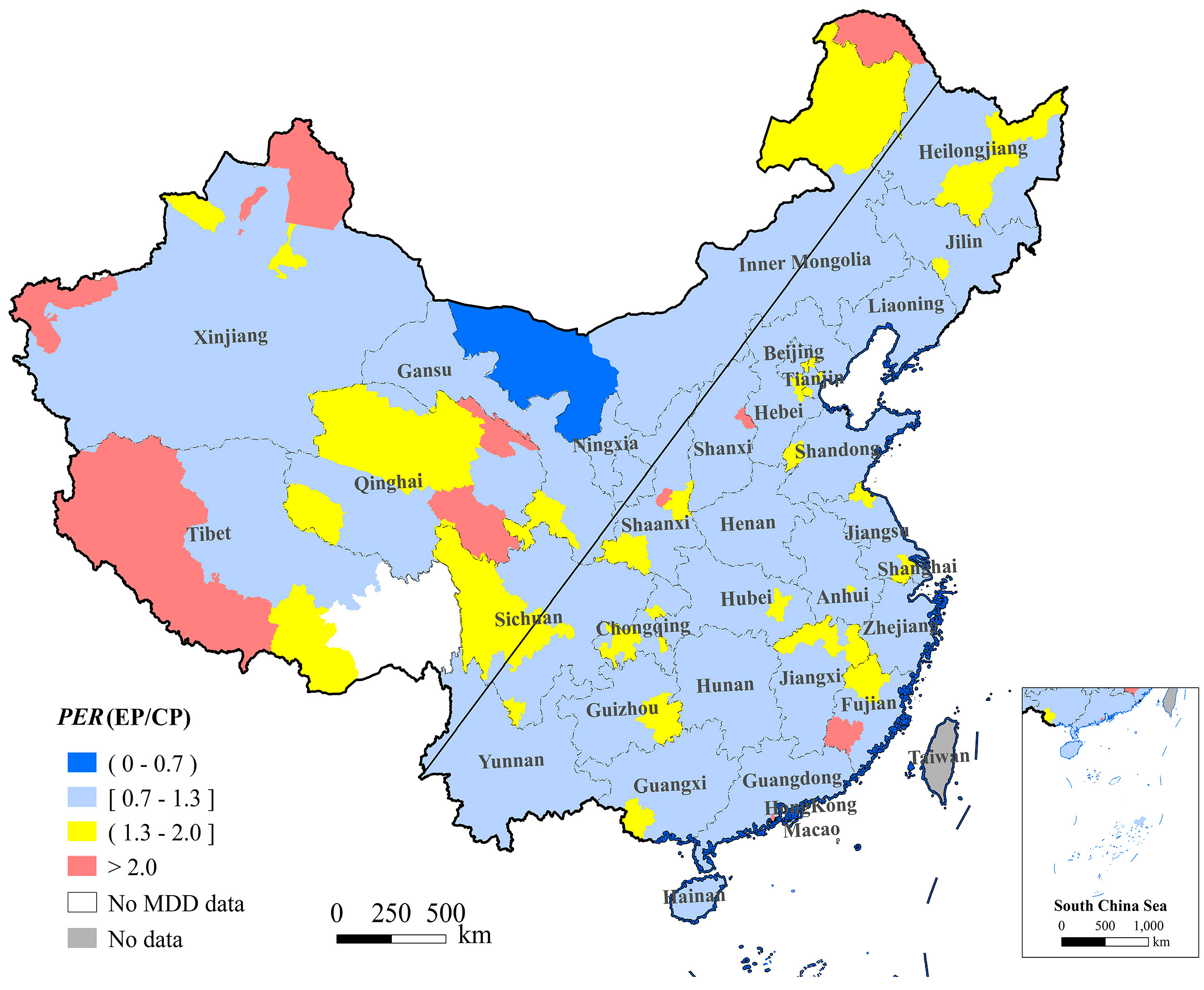
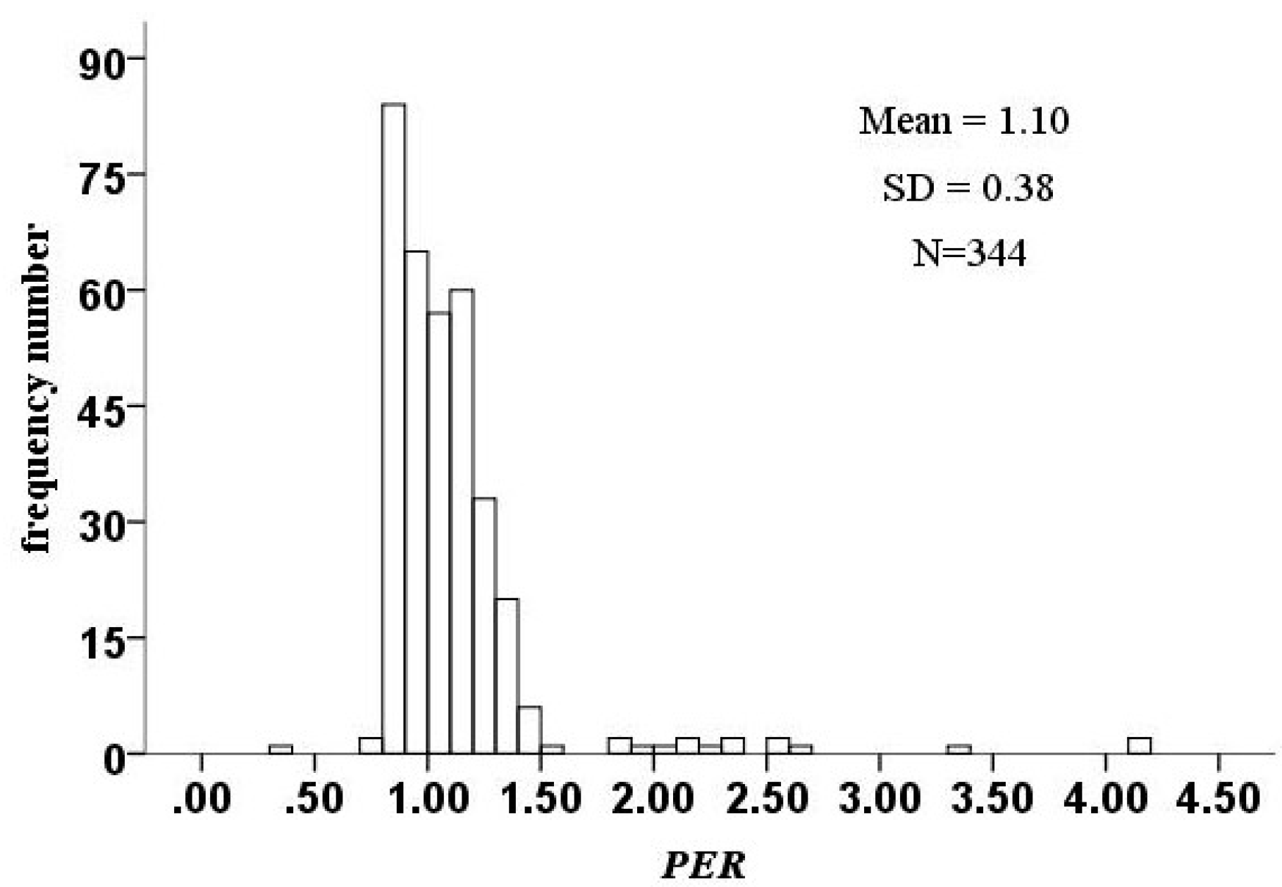
The total estimated urban population was 7.03 million, while census urban population was 6.70 million. The overall relative error was 4.9%. In order to evaluate the results, the estimated population was compared with the census population for each city. PER, the ratio of estimated urban population (EP) to census urban population (CP) (dividing the EP by the CP), was considered to be an index to evaluate the results for each city. Figure 4 shows the spatial distribution of PER. Table 4 shows the statistical information for PER. A total of 301 prefectures, distributed across almost all of China and accounting for 87.50% of the total prefectures, had PER values between 0.7~1.3. Only one city had PER values smaller than 0.7. The number of cites with PER values between 1.3 and 2.0 and larger 2.0 were 30 and 12, respectively, which was terribly overestimated, and mainly distributed in the north-east, north-west and south-west of China. Figure 5 shows the histogram of K. The mean = 1.10, SD = 0.38, and the distribution of PER was concentrated in the range 0.7–1.5. There were 151 prefectures with a PER less than 1.0, while 192 prefectures had a PER larger than 1.0.
Table 5 shows the number and percentage of cities in each PER range for region k. Generally, the number of cities with a PER between 0.7 and 1.3 reached 100% when k = 2, 3, 5. There were few cities overestimated in categories 1 and 4.
The number and percentage of cites in each PER range was also determined for different population levels (Table 6). It was found that the result was the poorest in level V, because there were only 66.67% of cities with a PER between 0.7 and 1.3, while the result was the best for level III. More than 80% of cities had a PER between 0.7 and 1.3 at levels I, II, and III. Thus, the method was applicable to levels I, II, III, and IV of cities, but inapplicable to level V of cities.
Differences between the estimated population and census population were mainly caused by the following. (1) Mdiffs data were extracted according to the land use data, and smaller areas of human settlement in the land use data led to a larger estimated population. (2) The quality of the DSM and DEM data directly affect the estimation result. Theoretically, the difference between the DSM and DEM data in non-human settlement areas should be 0 or small. However, the effects of terrain, vegetation, and water lead to abnormal differences in these areas, whereas the differences are normal in urban settlement areas. Many mountains are observed in north-western China and hills are observed in south-western China, and these regions host small scattered villages that are not accurately represented via land use data. This inaccuracy leads to lower MDD data values and larger estimated populations. (3) The census data based on the household registration principle cannot truly reflect the impact of population flows. (4) There is residual error in regression models. (5) Housing vacancies are caused by rapid urbanization; thus, new districts may present high vacancies or cities may be abandoned because of depleted resources. These cities are dark at night and mostly have high MDD values, which has led to higher estimated population values compared with the census population data.
The difference between the estimated population and census data is mainly caused by the accuracy of the datasets (land use data, DSM data, DEM data and census data), statistical methods and different building vacancy rates. Underestimation in most prefectural cities is mainly caused by regression models. With the development of LiDAR technology, more accurate DSM and DEM data will become available; thus, the population estimation results will be further improved. If the future DSM and DEM data for a region can be predicted based on the urban development conditions, the future population of the region can also be estimated. In addition, the spatial resolution of the estimation results can be improved according to the resolution of the land use data, which is an advantage compared to using night-time light data. Populations with a higher spatial resolution, such as 500 m, 300 m, or even 30 m, can be estimated if higher resolution land use data are used.
4. Conclusions
In this paper, the elevation difference between the DSM and DEM data was first calculated, and then the Mdiffs was extracted through land use data. Based on the MDD and CPD of the prefectural regions, China was divided into six region types using the adjusted box plot algorithm based on the K index; the regression functions through the origin between the MDD and CPD of the cities were then fitted. The urban population of China was estimated using these functions, and the results were compared with the census urban population. The results showed that a good linear correlation was found between the Mdiffs and the census data in each type of region, with all the adjusted R2 values above 0.9. The total estimated urban population of China in 2010 was close to the census population, but slightly overestimated. The results identified 301 prefectures, which accounts for 87.52% of the total number of prefectures in China, and the PER value was between 0.7 and 1.3.
The paper selected the K index to classify the study area through many tests. The character variables—CPD, MDD, and K—and their logarithms attempted to create different combinations. With regard to the classification algorithms, partitioning around medoids (k-medoids), affinity propagation (AP), average silhouette, and density-based spatial clustering of applications with noise (DBSCAN) were tested to confirm the optimum clustering number. However, only the results of the k-medoids method with the K index was appropriate. With regard to the hierarchical clustering, other linkage criteria methods were tried such as the maximum distance, median and Ward’s method. However, the Mcquitty method (using the Euclidean distance as a metric) was found to be the best (the best method was confirmed using the regression results and spatial distribution method).
This work used DSM and DEM data to estimate the urban population of China. Compared with population estimations using mobile phone data, the proposed method is simple and not limited by users and data privacy issues. Compared with previous work, this paper extracted height data with a 1 km resolution and regressed it with the census population directly at the prefectural city level instead of estimating the population with high resolution data for small areas (e.g., the downtown area of a city or a community). The estimated total urban population was very close to the census population. The study proved that height data can be used to estimate the regional population of large areas.
The difference between the estimated population and the census data was mainly caused by the accuracy of the datasets (land use data, DSM data, DEM data and census data), statistical methods, and different building vacancy rates. Underestimation in most of the prefectural cities was mainly caused by the regression models.
Author Contributions
Conceptualization, W.X. and L.Q.; Formal analysis, J.Z.; Investigation, J.Z.; Methodology, J.Z., W.X. and L.Q.; Writing—review & editing, J.Z., W.X. and Y.T.
Funding
This research was funded by the Ministry of Science and Technology of China, grant number 2016YFA0602404, and the National Natural Science Foundation of China, grant number 41571488/41201547 and the Ministry of Education and State Administration of Foreign Experts Affairs of China, grant number B08008
Acknowledgments
The authors are grateful to the editors and three anonymous reviewers for their critical comments and valuable suggestions, which helped to improve the quality of this manuscript substantially.
Conflicts of Interest
The authors declare no conflict of interest.
References
- UN Population Fund (UNFPA). “Report of the International Conference on Population and Development,” in Cairo, 5–13 September 1994, 1995, A/CONF.171/13/Rev.1. Available online: http://www.refworld.org/docid/4a54bc080.html (accessed on 11 September 2018).
- Coleman, D. The Twilight of the Census. Popul. Dev. Rev. 2013, 38, 334–351. [Google Scholar] [CrossRef] [Green Version]
- Ferrando, O. Manipulating the census: Ethnic minorities in the nationalizing states of Central Asia. Nationalities Pap. 2008, 36, 489–520. [Google Scholar] [CrossRef]
- Deville, P.; Linard, C.; Martin, S.; Gilbert, M.; Stevens, F.R.; Gaughan, A.E.; Blondel, V.D.; Tatem, A.J. Dynamic population mapping using mobile phone data. Proc. Natl. Acad. Sci. USA 2014, 111, 15888–15893. [Google Scholar] [CrossRef] [PubMed] [Green Version]
- Douglass, R.W.; Meyer, D.A.; Ram, M.; Rideout, D.; Song, D. High resolution population estimates from telecommunications data. EPJ Data Sci. 2015, 4. [Google Scholar] [CrossRef]
- Kang, C.; Liu, Y.; Ma, X.; Wu, L. Towards Estimating Urban Population Distributions from Mobile Call Data. J. Urban Technol. 2012, 19, 3–21. [Google Scholar] [CrossRef]
- Li, X.; Zhang, Y.Q.; Vasilakos, A.V. Discovering and predicting temporal patterns of wifi-interactive social populations. Comput. Sci. 2014, 99–122. [Google Scholar]
- Kontokosta, C.; Johnson, N. Urban phenology: Toward a real-time census of the city using Wi-Fi data. Comput. Environ. Urban Syst. 2017, 64, 144–153. [Google Scholar] [CrossRef]
- Kounadi, O.; Ristea, A.; Leitner, M.; Langford, C. Population at risk: Using areal interpolation and twitter messages to create population models for burglaries and robberies. Cartogr. Geogr. Inf. Sci. 2018, 45, 205–220. [Google Scholar] [CrossRef] [PubMed]
- Rich, A.J.; Lachowsky, N.J.; Sereda, P.; Cui, Z.; Wong, J.; Wong, S.; Jollimore, J. Estimating the size of the msm population in metro vancouver, canada, using multiple methods and diverse data sources. J. Urban Health. 2017, 95, 188–195. [Google Scholar] [CrossRef] [PubMed]
- Patel, N.N.; Stevens, F.R.; Huang, Z.; Gaughan, A.E.; Elyazar, I.; Tatem, A.J. Improving large area population mapping using geotweet densities. Trans. GIS. 2017, 21, 317–331. [Google Scholar] [CrossRef] [PubMed]
- Mellon, J.; Prosser, C. Twitter and facebook are not representative of the general population: Political attitudes and demographics of social media users. Res. Politics 2017, 4. [Google Scholar] [CrossRef]
- Liu, X.; Herold, M. Population Estimation and Interpolation Using Remote Sensing. In Urban Remote Sensing; CRC Press: Boca Raton, FL, USA, 2007; pp. 269–290. [Google Scholar]
- Wu, S.; Qiu, X.; Wang, L. Population Estimation Methods in GIS and Remote Sensing: A Review. GIsci. Remote Sens. 2005, 42, 80–96. [Google Scholar] [CrossRef]
- Azar, D.; Graesser, J.; Engstrom, R.; Comenetz, J.; Leddy, R.M., Jr.; Schechtman, N.G.; Andrews, T. Spatial refinement of census population distribution using remotely sensed estimates of impervious surfaces in Haiti. Int. J. Remote Sens. 2010, 31, 5635–5655. [Google Scholar] [CrossRef]
- Lam, N.S. Spatial Interpolation Methods: A Review. Cartogr. Geogr. Inf. Sci. 1983, 10, 129–150. [Google Scholar] [CrossRef]
- Mao, Y.; Ye, A.; Xu, J. Using Land Use Data to Estimate the Population Distribution of China in 2000. GISci. Remote Sens. 2012, 49, 822–853. [Google Scholar] [CrossRef]
- Gaughan, A.E.; Stevens, F.R.; Huang, Z.; Nieves, J.J.; Sorichetta, A.; Lai, S.; Ye, X.; Linard, C.; Hornby, G.M.; Hay, S.I.; et al. Spatiotemporal patterns of population in mainland China, 1990 to 2010. Sci. Data 2016, 3, 160005. [Google Scholar] [CrossRef] [PubMed] [Green Version]
- Lu, Z.; Im, J.; Quackenbush, L.J.; Halligan, K. Population estimation based on multi-sensor data fusion. Int. J. Remote Sens. 2010, 31, 5587–5604. [Google Scholar] [CrossRef]
- Dong, P.; Ramesh, S.; Nepali, A. Evaluation of small-area population estimation using LiDAR, Landsat TM and parcel data. Int. J. Remote Sens. 2010, 31, 5571–5586. [Google Scholar] [CrossRef]
- Alahmadi, M.; Atkinson, P.; Martin, D. Estimating the spatial distribution of the population of Riyadh, Saudi Arabia using remotely sensed built land cover and height data. Comput. Environ. Urban Syst. 2013, 41, 167–176. [Google Scholar] [CrossRef]
- Alahmadi, M.; Atkinson, P.; Martin, D. A Comparison of Small-Area Population Estimation Techniques Using Built-Area and Height Data, Riyadh, Saudi Arabia. IEEE J. Sel. Top. Appl. Earth Obs. Remote Sens. 2016, 9, 1959–1969. [Google Scholar] [CrossRef]
- Xie, Y.; Weng, A.; Weng, Q. Population Estimation of Urban Residential Communities Using Remotely Sensed Morphologic Data. IEEE Geosci. Remote Sens. Lett. 2015, 12, 1111–1115. [Google Scholar]
Figure 1.
Technical flow of the proposed method.

Figure 2.
Distribution of k.

Figure 3.
Distribution of the urban estimation and census population at the prefectural city level. (a) Estimated urban population size. (b) Census urban population size. (c) Estimated urban population density. (d) Census urban population density.
Figure 3.
Distribution of the urban estimation and census population at the prefectural city level. (a) Estimated urban population size. (b) Census urban population size. (c) Estimated urban population density. (d) Census urban population density.

Figure 4.
Distribution of PER (EP/CP).

Figure 5.
The histogram of PER (EP/CP).


Table 1.
Data used in this paper.
| Data | Time | Resolution | Source |
|---|---|---|---|
| DSM | 2008 | 30 m | Japan Aerospace Exploration Agency 1 |
| DEM | - | 1 arc-second/30 m | The National Aeronautics and Space Administration (NASA) of the United States 2 |
| Land Use | 2010 | 1 km/30 m | Institute of Geographic Sciences and Natural Resources, Chinese Academy of Sciences 3 |
| Census | 2010 | City level | National Bureau of Statistics of the People’s Republic of China 4 |
| Basic Geographic Information Data | 2004 | - | State Bureau of Surveying and Mapping, China |
Table 2.
The classification and regression results.
| Algorithms | Values Type | k | Sample Number | Adjusted R2 | Coefficient | SD of std. Residual |
|---|---|---|---|---|---|---|
| K-medoids | Normal values | 1 | 137 | 0.963 * | 1141.177 * | 0.999 |
| 2 | 88 | 0.984 * | 2394.861 * | 0.996 | ||
| 3 | 68 | 0.991 * | 3132.328 * | 0.939 | ||
| 4 | 35 | 0.999 * | 4931.935 * | 0.969 | ||
| Outliers | 5 | 15 | 0.982 * | 7012.809 * | 0.997 | |
| 6 | 1 | — | — | — | ||
| Box plot | Normal values | 1 | 86 | 0.970 * | 1118.123 * | 0.991 |
| 2 | 86 | 0.988 * | 1777.533 * | 0.999 | ||
| 3 | 86 | 0.992 * | 2684.094 * | 0.995 | ||
| 4 | 70 | 0.981 * | 4586.383 * | 0.954 | ||
| Outliers | 5 | 16 | 0.982 * | 7012.809 * | 0.997 | |
| Hierarchical clustering | Normal values | 1 | 103 | 0.970 * | 1119.915 * | 0.996 |
| 2 | 153 | 0.958 * | 2273.390 * | 1.000 | ||
| 3 | 72 | 0.980 * | 4568.570 * | 0.950 | ||
| Outliers | 4 | 12 | 0.989 * | 6882.477 * | 0.999 | |
| 5 | 3 | 0.950 | 8430.147 | 1.000 | ||
| 6 | 1 | — | — | — | ||
| Adjusted box plot | Normal values | 1 | 86 | 0.970 * | 1118.123 * | 0.991 |
| 2 | 86 | 0.988 * | 1777.533 * | 0.999 | ||
| 3 | 86 | 0.992 * | 2684.094 * | 0.995 | ||
| 4 | 70 | 0.981 * | 4586.383 * | 0.954 | ||
| Outliers | 5 | 12 | 0.997 * | 6641.906 * | 0.990 | |
| 6 | 4 | 0.994 * | 8910.301 * | 0.983 |
* Significant at the level of 0.05 (both sides).
Table 3.
The number (N) and percentage (P) of prefectures with different population size (PZ) and population density (PD) grades.
Table 3.
The number (N) and percentage (P) of prefectures with different population size (PZ) and population density (PD) grades.
| PZ grades (thousand) | EP | CP | PD Grades (person/km2) | EP | CP | ||||
|---|---|---|---|---|---|---|---|---|---|
| N | P (%) | N | P (%) | N | P (%) | N | P (%) | ||
| 0 | 2 | 0.58 | 0 | 0.00 | 0 | 2 | 0.58 | 0 | 0.00 |
| (0, 100] | 5 | 1.45 | 9 | 2.60 | (0, 50] | 84 | 24.28 | 89 | 25.72 |
| (100, 500] | 36 | 10.40 | 41 | 11.85 | (50, 100] | 64 | 18.50 | 68 | 19.65 |
| (500, 1000] | 73 | 21.10 | 76 | 21.97 | (100, 200] | 73 | 21.10 | 72 | 20.81 |
| (1000, 2000] | 112 | 32.37 | 113 | 32.66 | (200, 500] | 88 | 25.43 | 84 | 24.28 |
| (2000, 5000] | 94 | 27.17 | 86 | 24.86 | (500, 1000] | 22 | 6.36 | 23 | 6.65 |
| >5000 | 24 | 6.94 | 21 | 6.07 | >1000 | 13 | 3.76 | 10 | 2.89 |
Table 4.
The number and percentage of prefectures in each PER grade.
| PER Grades | Adjusted Box Plot | |
|---|---|---|
| Number of Cities | Percentage (%) | |
| (0, 0.7) | 1 | 0.29 |
| [0.7, 1.3] | 301 | 87.50 |
| (1.3, 2.0] | 30 | 8.72 |
| >2.0 | 12 | 3.49 |
Table 5.
The number (N) and percentage (P) of cities in each PER range for each k category.
| k | (0, 0.7) | [0.7, 1.3] | (1.3, 2.0] | >2.0 | ||||
|---|---|---|---|---|---|---|---|---|
| N | P (%) | N | P (%) | N | P (%) | N | P (%) | |
| 1 | 0 | 0.00 | 58 | 67.44 | 16 | 18.60 | 12 | 13.95 |
| 2 | 0 | 0.00 | 86 | 100.00 | 0 | 0.00 | 0 | 0.00 |
| 3 | 0 | 0.00 | 86 | 100.00 | 0 | 0.00 | 0 | 0.00 |
| 4 | 0 | 0.00 | 56 | 80.00 | 14 | 20.00 | 0 | 0.00 |
| 5 | 0 | 0.00 | 12 | 100.00 | 0 | 0.00 | 0 | 0.00 |
| 6 | 1 | 25.00 | 3 | 75.00 | 0 | 0.00 | 0 | 0.00 |
Table 6.
The number (N) and percentage (P) of cities in each PER range for each city level.
| City Level | Population (ten thousand) | (0, 0.7) | [0.7, 1.3] | (1.3, 2.0] | >2.0 | ||||
|---|---|---|---|---|---|---|---|---|---|
| N | P (%) | N | P (%) | N | P (%) | N | P (%) | ||
| I | >1000 | 0 | 0.00 | 4 | 80.00 | 1 | 20.00 | 0 | 0.00 |
| II | 500−1000 | 0 | 0.00 | 13 | 81.25 | 3 | 18.75 | 0 | 0.00 |
| III | 100−500 | 0 | 0.00 | 186 | 93.47 | 11 | 5.53 | 2 | 1.01 |
| IV | 50−100 | 0 | 0.00 | 66 | 86.84 | 9 | 11.84 | 1 | 1.32 |
| V | <50 | 1 | 2.08 | 32 | 66.67 | 6 | 12.50 | 9 | 18.75 |
© 2018 by the authors. Licensee MDPI, Basel, Switzerland. This article is an open access article distributed under the terms and conditions of the Creative Commons Attribution (CC BY) license (http://creativecommons.org/licenses/by/4.0/).
Share and Cite
MDPI and ACS Style
Zhang, J.; Xu, W.; Qin, L.; Tian, Y. Spatial Distribution Estimates of the Urban Population Using DSM and DEM Data in China. ISPRS Int. J. Geo-Inf. 2018, 7, 435. https://0-doi-org.brum.beds.ac.uk/10.3390/ijgi7110435
AMA Style
Zhang J, Xu W, Qin L, Tian Y. Spatial Distribution Estimates of the Urban Population Using DSM and DEM Data in China. ISPRS International Journal of Geo-Information. 2018; 7(11):435. https://0-doi-org.brum.beds.ac.uk/10.3390/ijgi7110435
Chicago/Turabian StyleZhang, Junlin, Wei Xu, Lianjie Qin, and Yugang Tian. 2018. "Spatial Distribution Estimates of the Urban Population Using DSM and DEM Data in China" ISPRS International Journal of Geo-Information 7, no. 11: 435. https://0-doi-org.brum.beds.ac.uk/10.3390/ijgi7110435
Note that from the first issue of 2016, this journal uses article numbers instead of page numbers. See further details here.