Landslide Susceptibility Mapping Using Logistic Regression Analysis along the Jinsha River and Its Tributaries Close to Derong and Deqin County, Southwestern China


Abstract
:1. Introduction
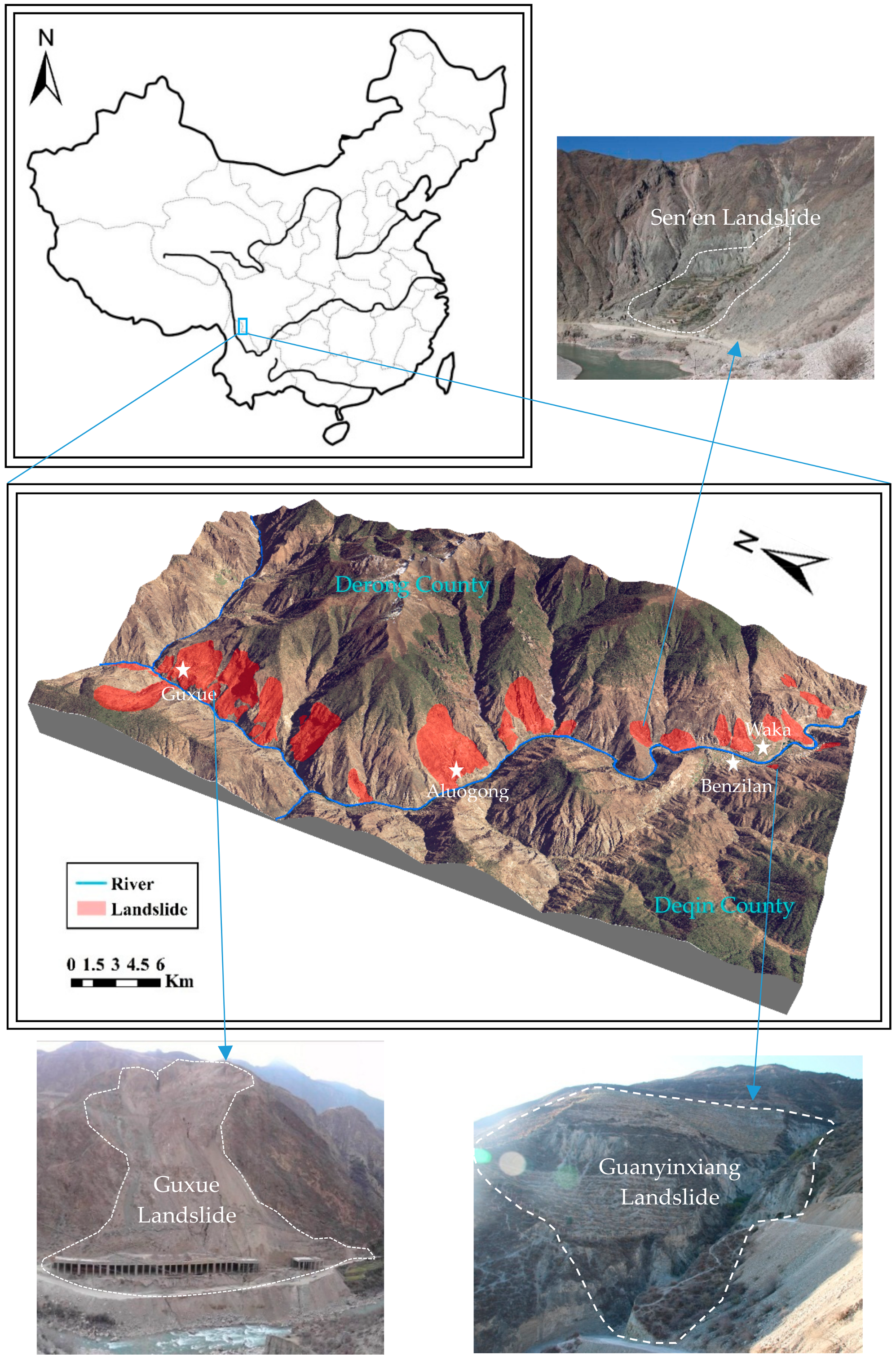
2. Study Area
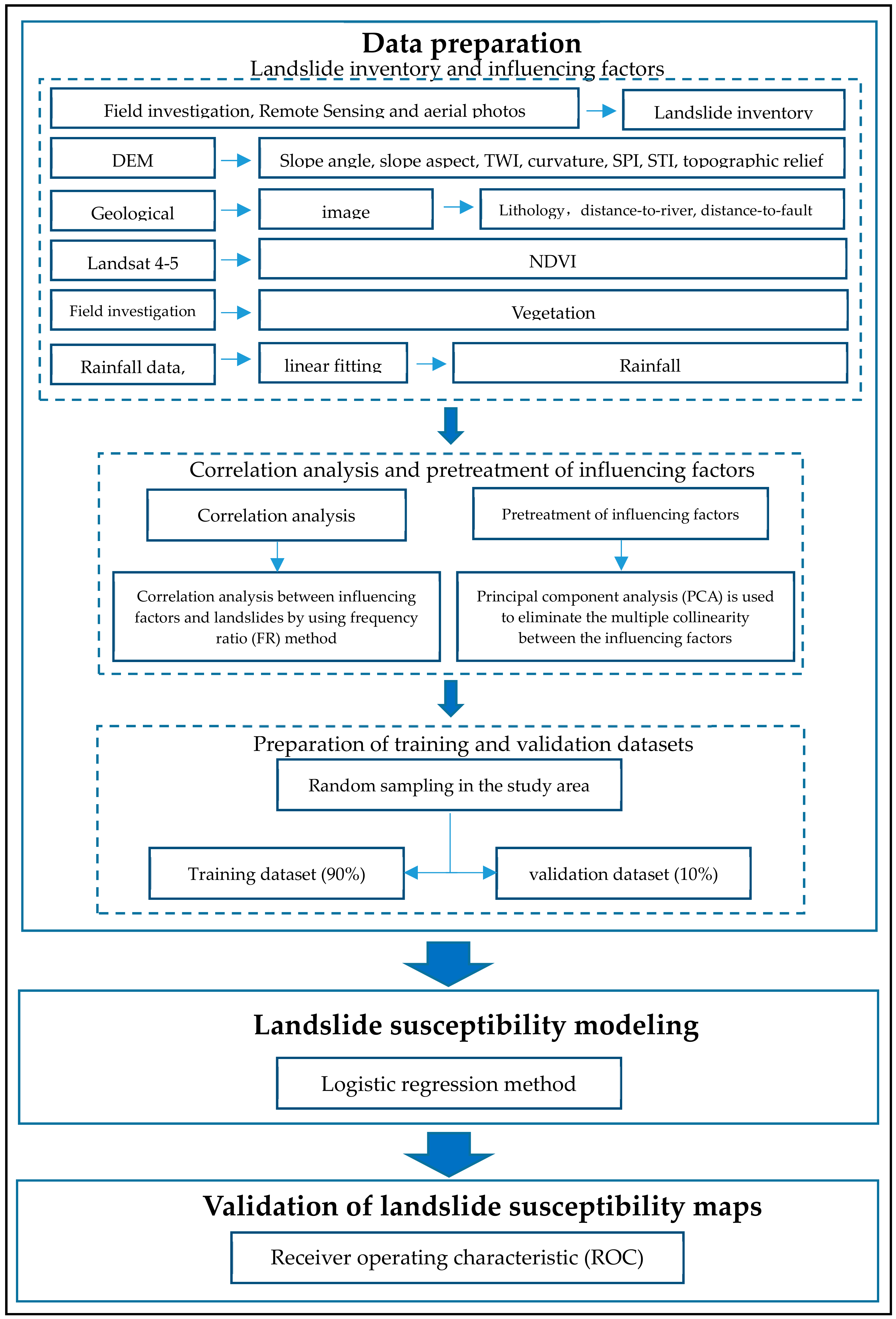
3. Methodology
3.1. Methods
3.2. Landslides and Influencing Factors
3.2.1. Landslide Inventory
3.2.2. Lithology Factor
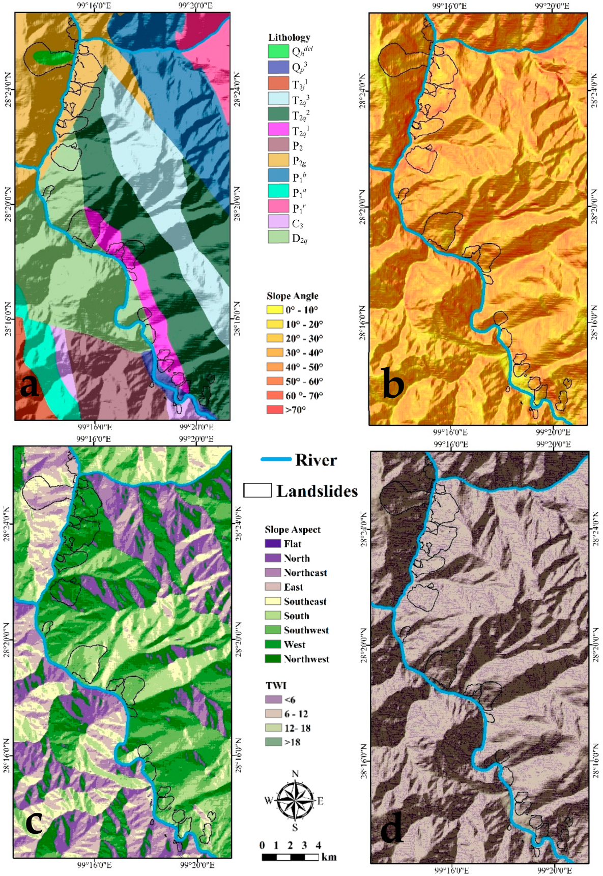
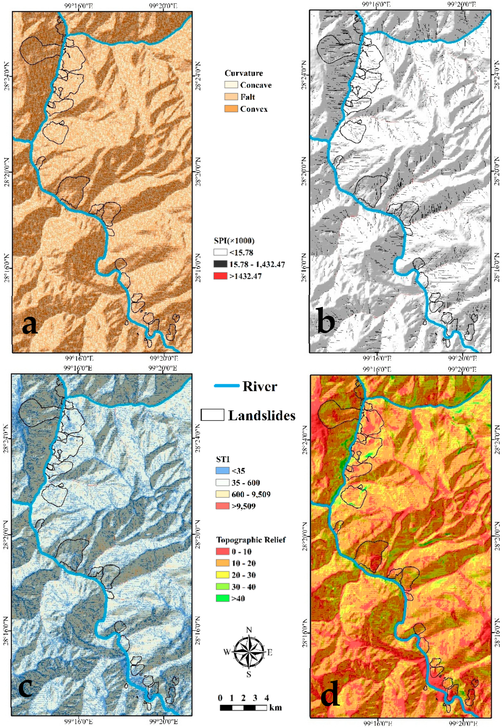
3.2.3. Geomorphological Factors
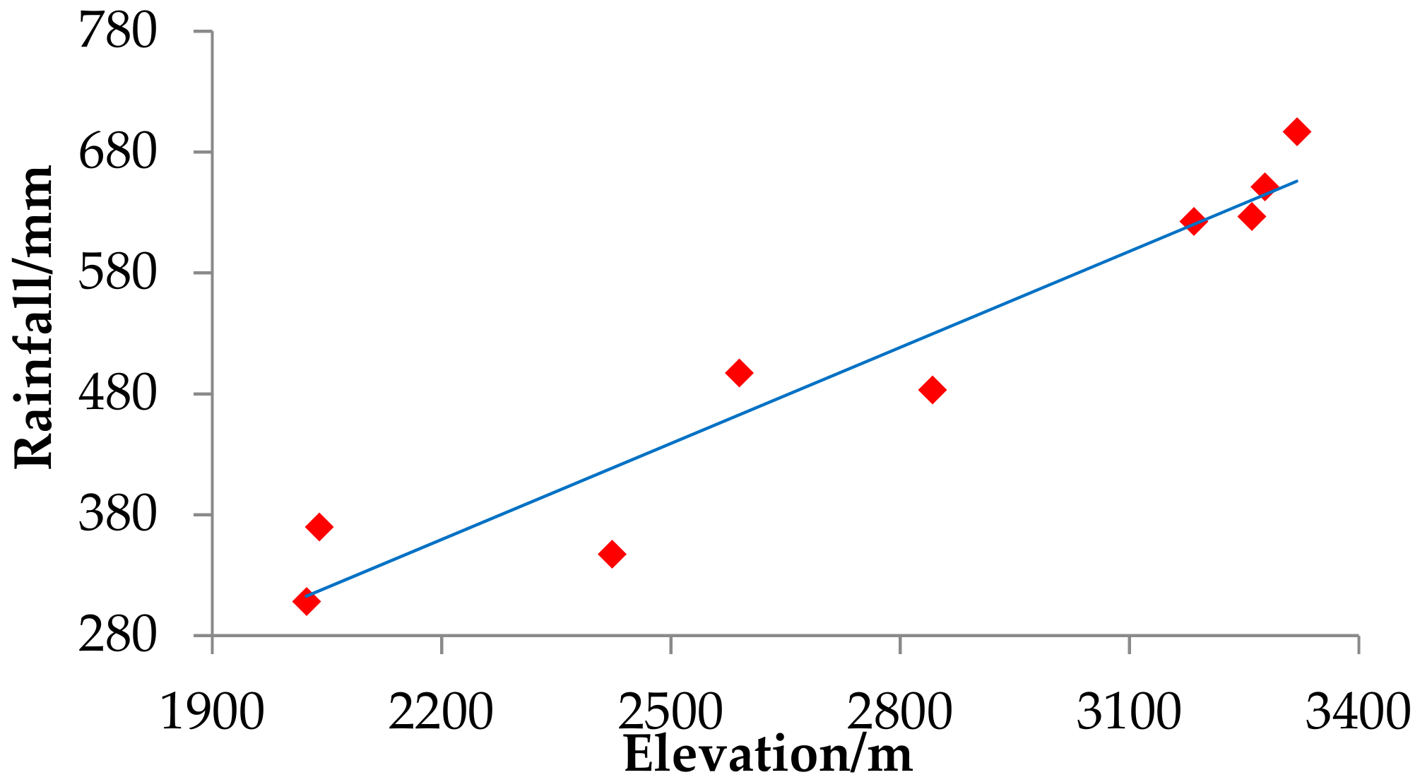
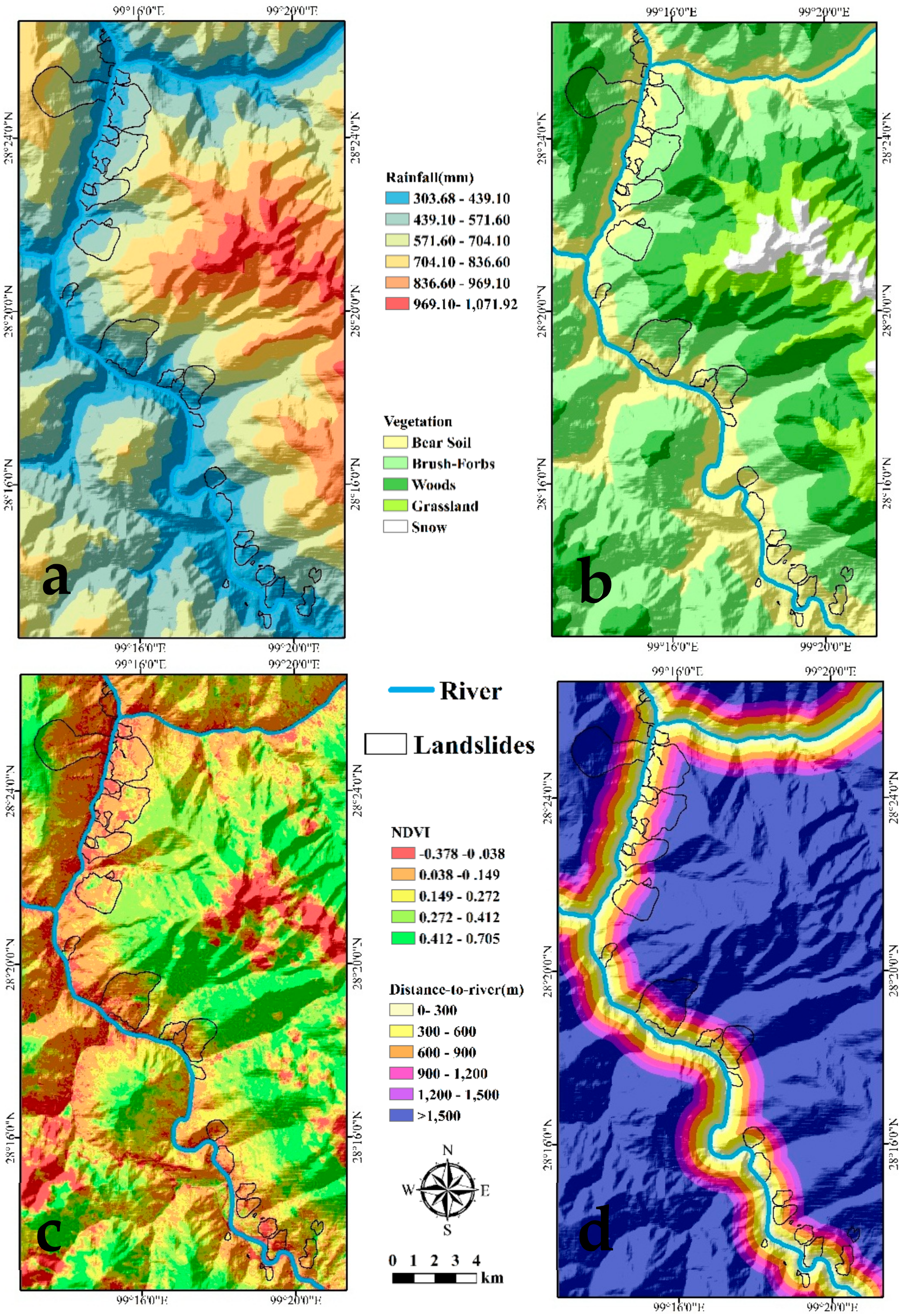
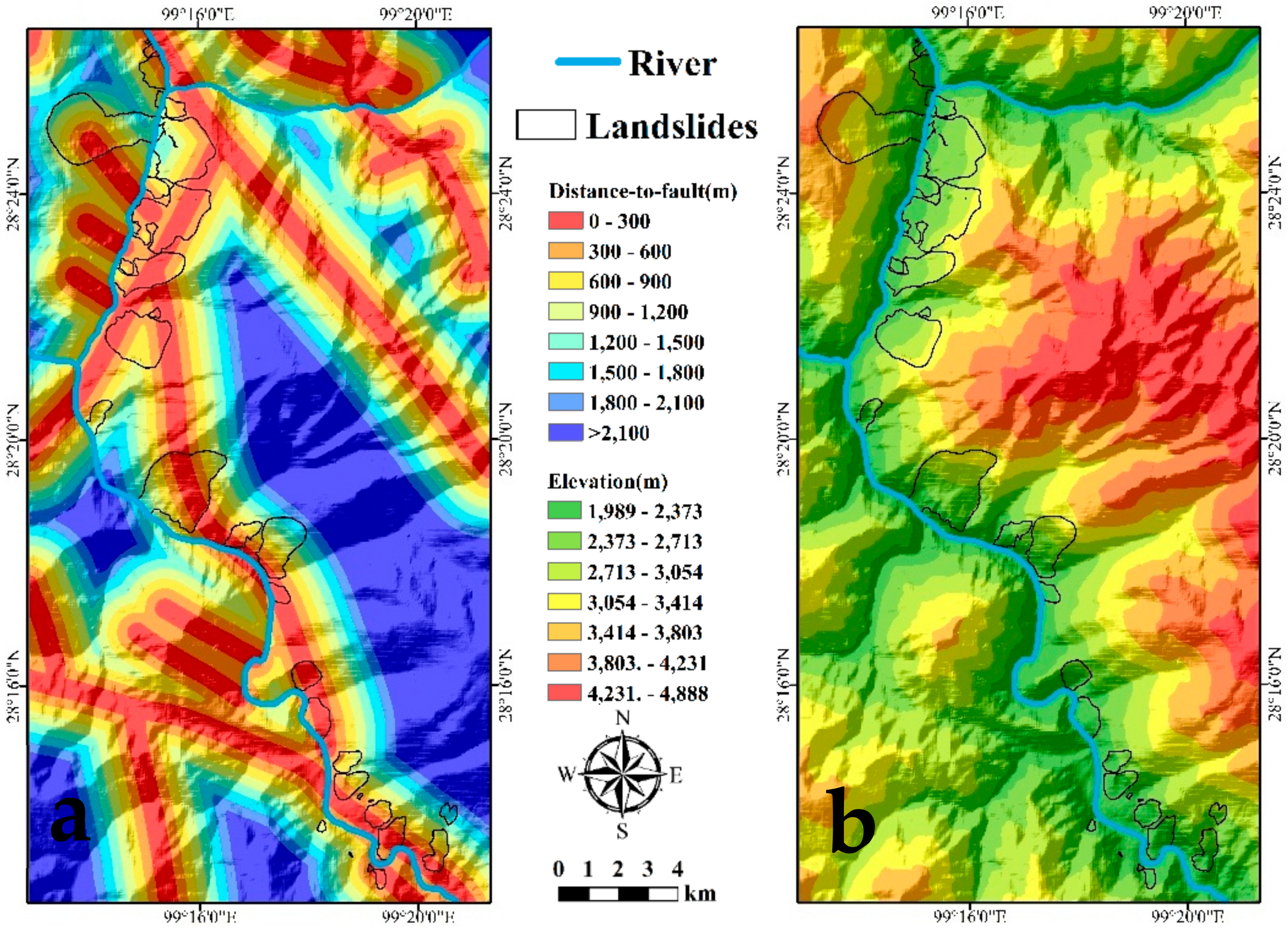
3.2.4. Environmental Factors
3.3. Evaluation of Influencing Factors
3.3.1. Probabilistic Relationship Analysis between Landslides and the Influencing Factors
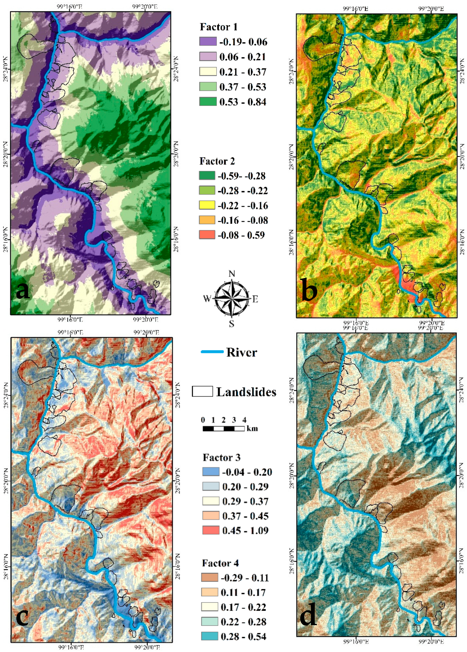
3.3.2. Principal Component Analysis
- (1)
- Use the following equation to normalize the preselected influencing factors:
- (2)
- In ArcGIS 10.2 software, a 20 × 20 m fishnet was built to sample 13 preselected factors.
- (3)
- Using the Kaiser–Meyer–Olkin (KMO) test and the Bartlett’s test of the sample data, the applicability of PCA can be verified.
- (4)
- PCA was carried out for the sample data, and a correlation matrix eigenvalue greater than 0.9 was selected as the principal component.
- (5)
- According to the principal component, a new influencing factors system will be built.
3.4. Data for the Logistic Regression Analysis
3.5. Model Development
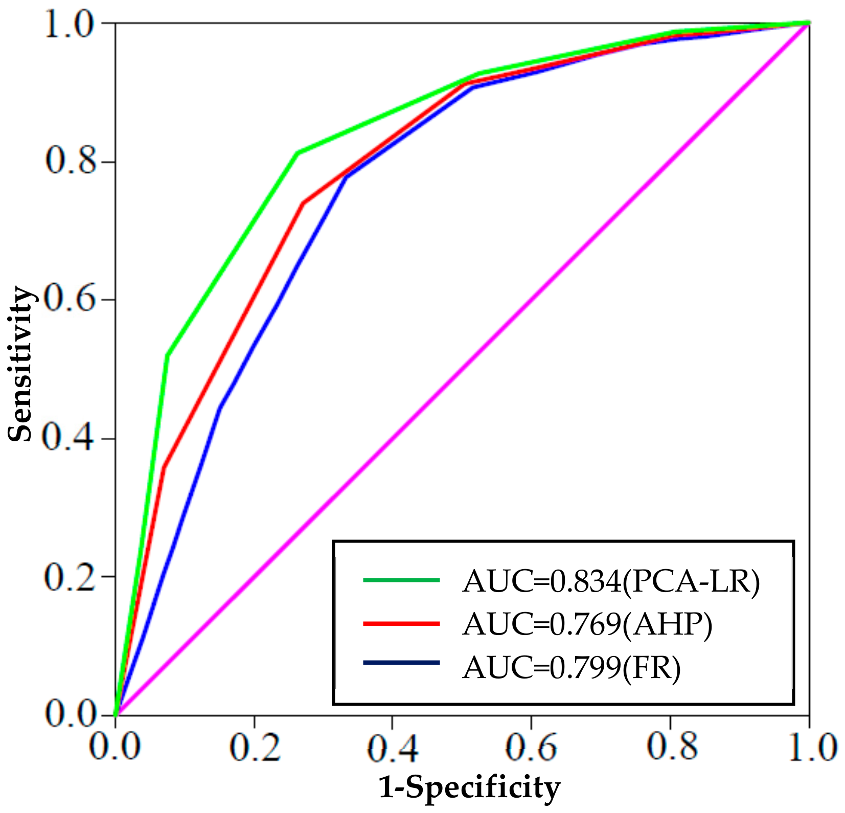
3.6. Model Validation
4. Results
4.1. Evaluation of Influencing Factors
4.2. Result of the PCA
4.3. Landslide Probability
5. Discussion
5.1. Validation
5.2. Key Factors for Landslide Occurrence
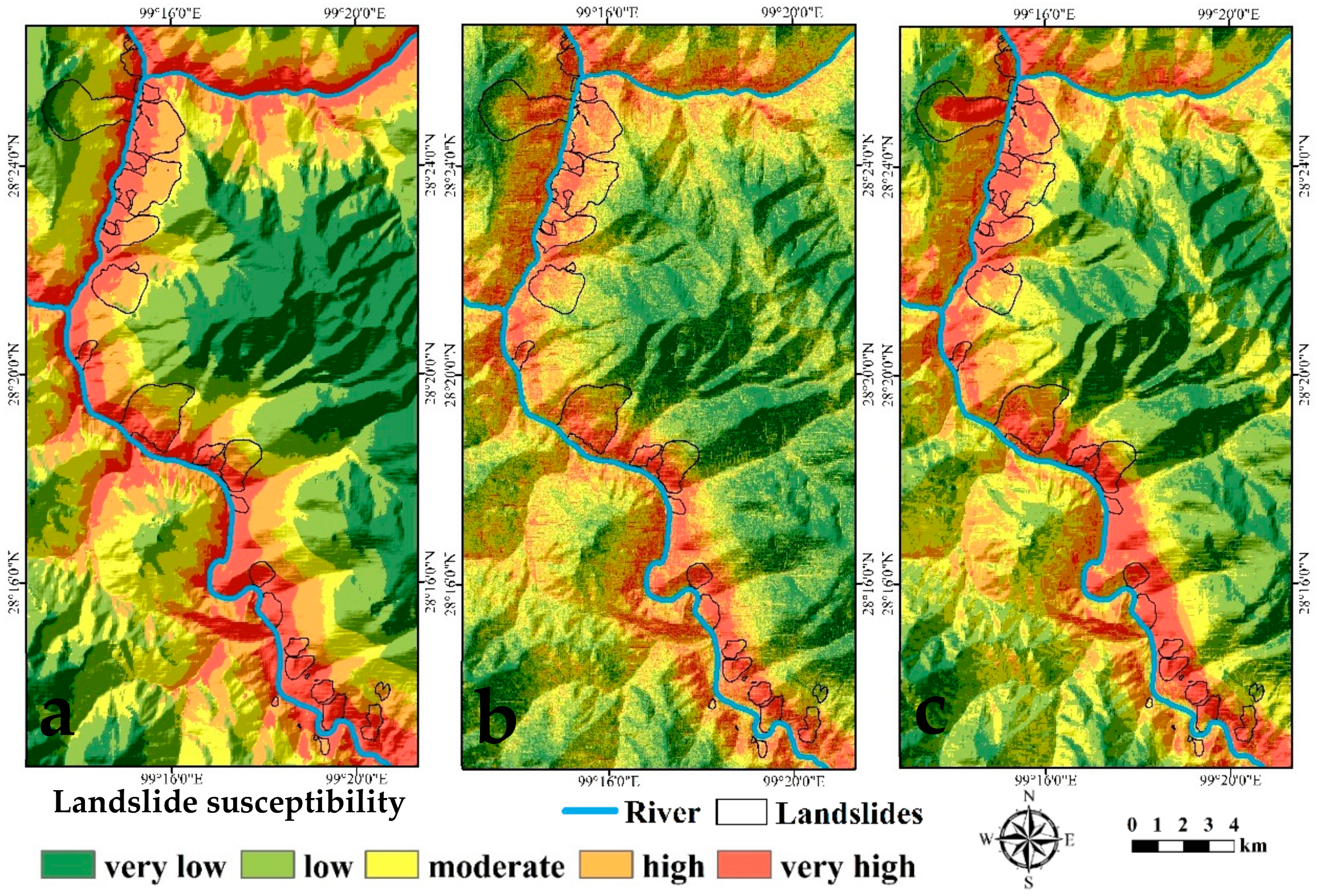
5.3. Landslide Susceptibility Mapping
6. Conclusions
Author Contributions
Funding
Acknowledgments
Conflicts of Interest
References
- Aleotti, P.; Chowdhury, R. Landslide hazard assessment: Summary review and new perspectives. Bull. Eng. Geol. Environ. 1999, 58, 21–44. [Google Scholar] [CrossRef]
- Saha, A.K.; Gupta, R.P.; Sarkar, I.; Arora, M.K.; Csaplovics, E. An approach for GIS-based statistical landslide susceptibility zonation—With a case study in the himalayas. Landslides 2005, 2, 61–69. [Google Scholar] [CrossRef]
- Fell, R.; Corominas, J.; Bonnard, C.; Cascini, L.; Leroi, E.; Savage, W.Z. Guidelines for landslide susceptibility, hazard and risk zoning for land use planning. Eng. Geol. 2008, 102, 85–98. [Google Scholar] [CrossRef] [Green Version]
- Guzzetti, F.; Reichenbach, P.; Ardizzone, F.; Cardinali, M.; Galli, M. Estimating the quality of landslide susceptibility models. Geomorphology 2006, 81, 166–184. [Google Scholar] [CrossRef]
- Raja, N.B.; Çiçek, I.; Türkoğlu, N.; Aydin, O.; Kawasaki, A. Correction to: Landslide susceptibility mapping of the sera river basin using logistic regression model. Nat. Hazards 2018, 91, 1423–1423. [Google Scholar] [CrossRef]
- Brabb, E.E.; Pampeyan, E.H.; Bonilla, M.G. Landslide Susceptibility in San Mateo County, California. Ph.D. Thesis, Stanford University, Stanford, CA, USA, 1972. [Google Scholar]
- Corominas, J.; Westen, C.V.; Frattini, P.; Cascini, L.; Malet, J.P.; Fotopoulou, S. Recommendations for the quantitative analysis of landslide risk. Bull. Eng. Geol. Environ. 2014, 73, 209–263. [Google Scholar] [CrossRef] [Green Version]
- Bai, S.B.; Wang, J.; Lü, G.N.; Zhou, P.G.; Hou, S.S.; Xu, S.N. Gis-based logistic regression for landslide susceptibility mapping of the zhongxian segment in the three gorges area, China. Geomorphology 2010, 115, 23–31. [Google Scholar] [CrossRef]
- Yesilnacar, E.; Topal, T. Landslide susceptibility mapping: A comparison of logistic regression and neural networks methods in a medium scale study, Hendek region (Turkey). Eng. Geol. 2005, 79, 251–266. [Google Scholar] [CrossRef]
- YïLmaz, I. Landslide susceptibility mapping using frequency ratio, logistic regression, artificial neural networks and their comparison: A case study from Kat landslides (Tokat-Turkey). Comput. Geosci. 2009, 35, 1125–1138. [Google Scholar] [CrossRef]
- Chen, W.; Pourghasemi, H.R.; Zhao, Z. A GIS-based comparative study of Dempster-Shafer, logistic regression and artificial neural network models for landslide susceptibility mapping. Geocarto Int. 2017, 32, 367–385. [Google Scholar] [CrossRef]
- Cao, C.; Xu, P.; Wang, Y.; Chen, J.; Zheng, L.; Niu, C. Flash flood hazard susceptibility mapping using frequency ratio and statistical index methods in coalmine subsidence areas. Sustainability 2016, 8, 948. [Google Scholar] [CrossRef]
- Chen, W.; Li, W.; Chai, H.; Hou, E.; Li, X.; Ding, X. GIS-based landslide susceptibility mapping using analytical hierarchy process (AHP) and certainty factor (CF) models for the Baozhong region of Baoji city, China. Environ. Earth Sci. 2016, 75, 1–14. [Google Scholar] [CrossRef]
- He, S.; Pan, P.; Dai, L.; Wang, H.; Liu, J. Application of kernel-based fisher discriminant analysis to map landslide susceptibility in the Qinggan river delta, Three Gorges, China. Geomorphology 2012, 171–172, 30–41. [Google Scholar] [CrossRef]
- Pourghasemi, H.R.; Rossi, M. Landslide susceptibility modeling in a landslide prone area in Mazandarn Province, north of Iran: A comparison between GLM, GAM, MARS, and M-AHP methods. Theor. Appl. Climatol. 2017, 130, 1–25. [Google Scholar] [CrossRef]
- Lombardo, L.; Bachofer, F.; Cama, M.; Märker, M.; Rotigliano, E. Exploiting maximum entropy method and aster data for assessing debris flow and debris slide susceptibility for the Giampilieri catchment (north-eastern Sicily, Italy). Earth Surf. Process. Landf. 2016, 41, 1776–1789. [Google Scholar] [CrossRef]
- Pham, B.T.; Bui, D.T.; Pourghasemi, H.R.; Indra, P.; Dholakia, M.B. Landslide susceptibility assesssment in the Uttarakhand area (India) using GIS: A comparison study of prediction capability of naive bayes, multilayer perceptron neural networks, and functional trees methods. Theor. Appl. Climatol. 2015, 122, 1–19. [Google Scholar] [CrossRef]
- Chen, W.; Pourghasemi, H.R.; Kornejady, A.; Zhang, N. Landslide spatial modeling: Introducing new ensembles of ANN, MaxEnt, and SVM machine learning techniques. Geocarto Int. 2017, 305, 314–327. [Google Scholar] [CrossRef]
- Lee, S.; Ryu, J.H.; Won, J.S.; Park, H.J. Determination and application of the weights for landslide susceptibility mapping using an artificial neural network. Eng. Geol. 2004, 71, 289–302. [Google Scholar] [CrossRef]
- Wang, E.; Burchfiel, B.C. Late Cenozoic to Holocene deformation in southwestern Sichuan and Adjacent. Yunnan, China, and its role in formation of the southeastern part of the Tibetan Plateau. Geol. Soc. Am. Bull. 2000, 112, 413–423. [Google Scholar] [CrossRef]
- Can, T.; Nefeslioglu, H.A.; Gokceoglu, C.; Sonmez, H.; Duman, T.Y. Susceptibility assessments of shallow earthflows triggered by heavy rainfall at three catchments by logistic regression analyses. Geomorphology 2005, 72, 250–227. [Google Scholar] [CrossRef]
- Guzzetti, F.; Mondini, A.C.; Cardinali, M.; Fiorucci, F.; Santangelo, M.; Chang, K.T. Landslide inventory maps: New tools for an old problem. Earth-Sci. Rev. 2012, 112, 42–66. [Google Scholar] [CrossRef]
- Yang, X.; Chen, L. Using multi-temporal remote sensor imagery to detect earthquake-triggered landslides. Int. J Appl. Earth Obs. 2010, 12, 487–495. [Google Scholar] [CrossRef] [Green Version]
- Cao, C.; Wang, Q.; Chen, J.; Ruan, Y.; Zheng, L.; Song, S.; Niu, C. Landslide susceptibility mapping in vertical distribution law of precipitation area: Case of the Xulong hydropower station reservoir, Southwestern China. Water 2016, 8, 270. [Google Scholar] [CrossRef]
- Wang, F.; Xu, P.; Wang, C.; Wang, N.; Jiang, N. Application of a GIS-based slope unit method for landslide susceptibility mapping along the Longzi river, southeastern Tibetan plateau, China. ISPRS Int. J. Geo-Inf. 2017, 6, 172. [Google Scholar] [CrossRef]
- Li, J.; Wang, C.; Wang, G.; Liu, W. Analysis of landslide influential factors and coupling intensity based on third theory of quantification. Chin. J. Rock Mech. Eng. 2010, 29, 1206–1213. [Google Scholar]
- Li, J.-X.; Wang, C.M.; Wang, G.C. Landslide risk assessment based on combination weighting-unascertained measure theory. Rock Soil Mech. 2013, 34, 468–474. [Google Scholar]
- Marjanović, M.; Kovačević, M.; Bajat, B.; Voženílek, V. Landslide susceptibility assessment using SVM machine learning algorithm. Eng. Geol. 2011, 123, 225–234. [Google Scholar] [CrossRef]
- Kanungo, D.P.; Arora, M.K.; Sarkar, S.; Gupta, R.P. A comparative study of conventional, ANN black box, fuzzy and combined neural and fuzzy weighting procedures for landslide susceptibility zonation in Darjeeling Himalayas. Eng. Geol. 2006, 85, 347–366. [Google Scholar] [CrossRef]
- Yalcin, A. GIS-based landslide susceptibility mapping using analytical hierarchy process and bivariate statistics in Ardesen (Turkey): Comparisons of results and confirmations. Catena 2008, 72, 1–12. [Google Scholar] [CrossRef]
- Akgun, A.; Sezer, E.A.; Nefeslioglu, H.A.; Gokceoglu, C.; Pradhan, B. An easy-to-use Matlab program (Mamland) for the assessment of landslide susceptibility using a Mamdani fuzzy algorithm. Comput. Geosci. 2012, 38, 23–34. [Google Scholar] [CrossRef]
- Mohammady, M.; Pourghasemi, H.R.; Pradhan, B. Landslide susceptibility mapping at Golestan province, Iran: A comparison between frequency ratio, dempster–shafer, and weights-of-evidence models. J. Asian Earth Sci. 2012, 61, 221–236. [Google Scholar] [CrossRef]
- Lee, S.; Min, K. Statistical analysis of landslide susceptibility at Yongin, Korea. Environ. Geol. 2001, 40, 1095–1113. [Google Scholar] [CrossRef]
- Simons, M. The Morphological Analysis of Landforms: A New Review of the Work of Walther Penck (1888–1923); JSTOR: New York, NY, USA, 1962. [Google Scholar]
- Conforti, M.; Pascale, S.; Robustelli, G.; Sdao, F. Evaluation of prediction capability of the artificial neural networks for mapping landslide susceptibility in the Turbolo river catchment (Northern Calabria, Italy). Catena 2014, 113, 236–250. [Google Scholar] [CrossRef]
- Hungr, O.; Leroueil, S.; Picarelli, L. The varnes classification of landslide types, an update. Landslides 2014, 11, 167–194. [Google Scholar] [CrossRef]
- Ozdemir, A. Using a binary logistic regression method and GIS for evaluating and mapping the groundwater spring potential in the Sultan Mountains (Aksehir, Turkey). J. Hydrol. 2011, 405, 123–136. [Google Scholar] [CrossRef]
- Gokceoglu, C.; Sonmez, H.; Nefeslioglu, H.A.; Duman, T.Y.; Can, T. The 17 March 2005 Kuzulu Landslide (Sivas, Turkey) and landslide-susceptibility map of its near vicinity. Eng. Geol. 2005, 81, 65–83. [Google Scholar] [CrossRef]
- Beven, K.; Kirkby, M.J. A physically based, variable contributing area model of basin hydrology. Hydrol. Sci. Bull. 1979, 24, 43–69. [Google Scholar] [CrossRef]
- Moore, I.D.; Burch, G.J. Physical Basis of the Length-slope Factor in the Universal Soil Loss Equation. Soil Sci. Soc. Am. J. 1986, 50, 1294–1298. [Google Scholar] [CrossRef]
- Oh, H.J.; Pradhan, B. Application of a neuro-fuzzy model to landslide-susceptibility mapping for shallow landslides in a tropical hilly area. Comput. Geosci. 2011, 37, 1264–1276. [Google Scholar] [CrossRef]
- Jebur, M.N.; Pradhan, B.; Tehrany, M.S. Optimization of landslide conditioning factors using very high-resolution airborne laser scanning (lidar) data at catchment scale. Remote Sens. Environ. 2014, 152, 150–165. [Google Scholar] [CrossRef]
- Moore, I.D.; Grayson, R.B.; Ladson, A.R. Digital terrain modelling: A review of hydrological, geomorphological, and biological applications. Hydrol. Process. 1991, 5, 3–30. [Google Scholar] [CrossRef]
- Pradhan, A.M.S.; Kang, H.S.; Lee, S.; Kim, Y.T. Spatial model integration for shallow landslide susceptibility and its runout using a GIS-based approach in Yongin, Korea. Geocarto Int. 2016, 32, 420–441. [Google Scholar] [CrossRef]
- Cheng, Q.; Ko, C.; Yuan, Y.; Ge, Y.; Zhang, S. GIS modeling for predicting river runoff volume in ungauged drainages in the greater Toronto area, Canada. Comput. Geosci. 2006, 32, 1108–1119. [Google Scholar] [CrossRef]
- Huang, Y.; Chen, S.; Cao, Q.; Hong, Y.; Wu, B.; Huang, M.; Qiao, L.; Zhang, Z.; Li, Z.; Li, W.; et al. Evaluation of version-7 TRMM multi-satellite precipitation analysis product during the Beijing extreme heavy rainfall event of 21 July 2012. Water 2013, 6, 32–44. [Google Scholar] [CrossRef]
- Park, S.; Choi, C.; Kim, B.; Kim, J. Landslide susceptibility mapping using frequency ratio, analytic hierarchy process, logistic regression, and artificial neural network methods at the Inje area, Korea. Environ. Earth Sci. 2013, 68, 1443–1464. [Google Scholar] [CrossRef]
- Hong, H.; Pradhan, B.; Xu, C.; Bui, D.T. Spatial prediction of landslide hazard at the Yihuang area (China) using two-class kernel logistic regression, alternating decision tree and support vector machines. Catena 2015, 133, 266–281. [Google Scholar] [CrossRef]
- Laxton, J. Geographic information systems for geoscientists—Modelling with GIS—Bonhamcarter, GF. Int. J. Geogr. Inf. Syst. 1996, 10, 355–356. [Google Scholar] [CrossRef]
- Hosmer, D.W., Jr.; Lemeshow, S.; Sturdivant, R.X. Applied Logistic Regression, 3rd ed.; John Wiley: Hoboken, NJ, USA, 2013. [Google Scholar]
- Djeddaoui, F.; Chadli, M.; Gloaguen, R.; Djeddaoui, F.; Chadli, M.; Gloaguen, R. Desertification susceptibility mapping using logistic regression analysis in the Djelfa area, Algeria. Remote Sens. 2017, 9, 1031. [Google Scholar] [CrossRef]
- Agterberg, F.P.; Cheng, Q. Conditional independence test for weights-of-evidence modeling. Nat. Resour. Res. 2002, 11, 249–255. [Google Scholar] [CrossRef]
- Preisendorfer, R.W.; Mobley, C.D. Principal component analysis in meteorology and oceanography. Dev. Atmos. Sci. 1988, 17, 55–72. [Google Scholar]
- Dai, F.C.; Lee, C.F. Landslide characteristics and slope instability modeling using GIS, Lantau Island, Hong Kong. Geomorphology 2002, 42, 213–228. [Google Scholar] [CrossRef]
- Bewick, V.; Cheek, L.; Ball, J. Statistics review 14: Logistic regression. Crit. Care 2005, 9, 112–118. [Google Scholar] [CrossRef] [PubMed]
- Regmi, N.R.; Giardino, J.R.; McDonald, E.V.; Vitek, J.D. A comparison of logistic regression-based models of susceptibility to landslides in Western Colorado, USA. Landslides 2014, 11, 247–262. [Google Scholar] [CrossRef]
- Clark, W.; Hosking, P. Statistical Methods for Geographers; John Wiley & Sons: New York, NY, USA, 1986. [Google Scholar]
- Mathew, J.; Jha, V.K.; Rawat, G.S. Landslide susceptibility zonation mapping and its validation in part of Garhwal Lesser Himalaya, India, using binary logistic regression analysis and receiver operating characteristic curve method. Landslides 2009, 6, 17–26. [Google Scholar] [CrossRef]
- Othman, A.A.; Gloaguen, R.; Andreani, L.; Rahnama, M. Landslide susceptibility mapping in Mawat area, Kurdistan Region, NE Iraq: A comparison of different statistical models. Nat. Hazards Earth Syst. Sci. Discuss. 2015, 3, 1789–1833. [Google Scholar] [CrossRef]
- Devkota, K.C.; Regmi, A.D.; Pourghasemi, H.R.; Yoshida, K.; Pradhan, B.; Ryu, I.C.; Dhital, M.R.; Althuwaynee, O.F. Landslide susceptibility mapping using certainty factor, index of entropy and logistic regression models in GIS and their comparison at Mugling–Narayanghat road section in Nepal Himalaya. Nat. Hazards 2013, 65, 135–165. [Google Scholar] [CrossRef] [Green Version]
- Lee, S. Application of logistic regression model and its validation for landslide susceptibility mapping using GIS and remote sensing data. Int. J. Remote Sens. 2005, 26, 1477–1491. [Google Scholar] [CrossRef]
- Hosmer, D.W., Jr.; Lemeshow, S.; Sturdivant, R.X. Model-building strategies and methods for logistic regression. In Applied Logistic Regression, 3rd ed.; Wiley: Hoboken, NJ, USA, 2000; pp. 89–151. [Google Scholar]
- Alatorre, L.C.; Sánchez-Andrés, R.; Cirujano, S.; Beguería, S.; Sánchez-Carrillo, S. Identification of mangrove areas by remote sensing: The ROC curve technique applied to the northwestern Mexico coastal zone using Landsat imagery. Remote Sens. 2011, 3, 1568–1583. [Google Scholar] [CrossRef] [Green Version]
- Chen, Y.; Booth, D.C. The Wenchuan Earthquake of 2008: Anatomy of a Disaster; Springer Science & Business Media: New York, NY, USA, 2011. [Google Scholar]
- Hao, M.; Wang, Q.; Shen, Z.; Cui, D.; Ji, L.; Li, Y.; Qin, S. Present day crustal vertical movement inferred from precise leveling data in eastern margin of Tibetan plateau. Tectonophysics 2014, 632, 281–292. [Google Scholar] [CrossRef]
- Burbank, D.W.; Leland, J.; Fielding, E.; Anderson, R.S.; Brozovic, N.; Reid, M.R.; Duncan, C. Bedrock incision, rock uplift and threshold hillslopes in the northwestern Himalayas. Nature 1996, 379, 505–510. [Google Scholar] [CrossRef]
- Pradhan, A.M.S.; Kim, Y.T. Relative effect method of landslide susceptibility zonation in weathered granite soil: A case study in Deokjeok-ri Creek, South Korea. Nat. Hazards 2014, 72, 1189–1217. [Google Scholar] [CrossRef]


| Precipitation Station | Longitude | Latitude | Elevation/m | Average Annual Precipitation/mm | Data Resources/Year |
|---|---|---|---|---|---|
| Derong | 99°10.2′ | 28°25.8′ | 2422.9 | 347.1 | 1981−2010 |
| Batang | 99°03.6′ | 30°00.0′ | 2589.2 | 497.0 | 1981−2010 |
| Xiangcheng | 99°28.8′ | 28°33.6′ | 2842.0 | 483.1 | 1981−2010 |
| Xianggelila | 99°25.2′ | 27°30.0′ | 3276.7 | 651.1 | 1981−2010 |
| Deqin | 98°33.0′ | 28°17.4′ | 3319.0 | 696.7 | 1981−2010 |
| Dege | 98°35.0′ | 31°48.0′ | 3184.0 | 622.4 | 1981−2010 |
| Baiyu | 98°50.0′ | 31°13.0′ | 3260.0 | 626.6 | 1981−2010 |
| Benilan | 99°17.0′ | 28°17.0′ | 2023.0 | 308.0 | 1965−1998 |
| Shangqiaotou | 99°24.0′ | 28°10.0′ | 2040.0 | 369.7 | 1961−2004 |
| Factors | Class | Landslide Not Occurred | Landslide Occurred | Total Count | FR | ||
|---|---|---|---|---|---|---|---|
| Count | Ratio | Count | Ratio | ||||
| Lithology | Qhdel | 1067 | 0.03% | 19,379 | 7.32% | 20,446 | 13.04 |
| Q3p | 44,741 | 1.33% | 4964 | 1.88% | 49,705 | 1.37 | |
| T3j1 | 82,644 | 2.45% | 0 | 0.00% | 82,644 | 0.00 | |
| T2q3 | 433,458 | 12.84% | 0 | 0.00% | 433,458 | 0.00 | |
| T2q2 | 646,006 | 19.13% | 37,075 | 14.00% | 683,081 | 0.75 | |
| T2q1 | 88,043 | 2.61% | 46,056 | 17.40% | 134,099 | 4.72 | |
| P2 | 265,722 | 7.87% | 639 | 0.24% | 266,361 | 0.03 | |
| P2g | 430,106 | 12.74% | 94,434 | 35.67% | 524,540 | 2.48 | |
| P1b | 461,126 | 13.66% | 0 | 0.00% | 461,126 | 0.00 | |
| P1a | 127,972 | 3.79% | 0 | 0.00% | 127,972 | 0.00 | |
| P1r | 141,015 | 4.18% | 0 | 0.00% | 141,015 | 0.00 | |
| C3 | 55,805 | 1.65% | 1763 | 0.67% | 57,568 | 0.42 | |
| D2q | 598,585 | 17.73% | 60,422 | 22.82% | 659,007 | 1.26 | |
| Slope Angle | 0–10 | 99,022 | 2.93% | 3832 | 1.45% | 102,854 | 0.51 |
| 10–20 | 390,709 | 11.57% | 27,926 | 10.55% | 418,635 | 0.92 | |
| 20–30 | 1,105,152 | 32.73% | 96,973 | 36.63% | 1,202,125 | 1.11 | |
| 30–40 | 1,284,364 | 38.04% | 105,990 | 40.04% | 1,390,354 | 1.05 | |
| 40–50 | 430,872 | 12.76% | 25,518 | 9.64% | 456,390 | 0.77 | |
| 50–60 | 60,726 | 1.80% | 3549 | 1.34% | 64,275 | 0.76 | |
| 60–70 | 5331 | 0.16% | 939 | 0.35% | 6270 | 2.06 | |
| >70 | 114 | 0.00% | 5 | 0.00% | 119 | 0.58 | |
| Slope Aspect | Flat | 1938 | 0.06% | 6 | 0.00% | 1944 | 0.04 |
| N | 433,950 | 12.85% | 7207 | 2.72% | 441,157 | 0.22 | |
| NE | 364,642 | 10.80% | 13,411 | 5.07% | 378,053 | 0.49 | |
| E | 387,480 | 11.48% | 28,779 | 10.87% | 416,259 | 0.95 | |
| SE | 340,425 | 10.08% | 14,563 | 5.50% | 354,988 | 0.56 | |
| S | 435,604 | 12.90% | 31,770 | 12.00% | 467,374 | 0.93 | |
| SW | 466,658 | 13.82% | 60,966 | 23.03% | 527,624 | 1.59 | |
| W | 509,216 | 15.08% | 67,252 | 25.40% | 576,468 | 1.60 | |
| NW | 436,377 | 12.92% | 40,778 | 15.40% | 477,155 | 1.18 | |
| TWI | <6 | 812,439 | 24.06% | 58,599 | 22.14% | 871,038 | 0.93 |
| 6–12 | 2,486,604 | 73.65% | 197,698 | 74.68% | 2,684,302 | 1.01 | |
| 12–18 | 70,336 | 2.08% | 8122 | 3.07% | 78,458 | 1.42 | |
| >18 | 6911 | 0.20% | 313 | 0.12% | 7224 | 0.60 | |
| Curvature | Concave | 1,341,951 | 39.75% | 105,133 | 39.71% | 1,447,084 | 1.00 |
| Flat | 689,221 | 20.41% | 55,595 | 21.00% | 744,816 | 1.03 | |
| Convex | 1,345,078 | 39.84% | 104,044 | 39.30% | 1,449,122 | 0.99 | |
| SPI (×104) | <15.78 | 1,029,734 | 30.50% | 2,447,736 | 93.58% | 3,477,470 | 0.98 |
| 15.78–1432.47 | 138,638 | 4.11% | 16,422 | 6.20% | 155,060 | 1.46 | |
| >1432.47 | 7898 | 0.23% | 574 | 0.22% | 8472 | 0.93 | |
| STI | <35 | 887,114 | 26.27% | 60,897 | 23.00% | 948,011 | 0.88 |
| 35–600 | 2,320,987 | 68.74% | 185,085 | 69.91% | 2,506,072 | 1.02 | |
| 600–9509 | 162,241 | 4.81% | 18,227 | 6.89% | 180,468 | 1.39 | |
| >9509 | 5948 | 0.18% | 523 | 0.20% | 6471 | 1.11 | |
| Topographic Relief | 0–10 | 707,752 | 20.96% | 52,211 | 19.72% | 759,963 | 0.94 |
| 10–20 | 2,052,327 | 60.79% | 170,331 | 64.34% | 2,222,658 | 1.05 | |
| 20–30 | 552,583 | 16.37% | 37,517 | 14.17% | 590,100 | 0.87 | |
| 30–40 | 54,636 | 1.62% | 2928 | 1.11% | 57,564 | 0.70 | |
| >40 | 8992 | 0.27% | 1745 | 0.66% | 10,737 | 2.24 | |
| Rainfall | 303.68–439.10 | 684,222 | 20.27% | 120,189 | 45.40% | 804,411 | 2.05 |
| 439.10–571.60 | 940,470 | 27.86% | 93,156 | 35.19% | 1,033,626 | 1.24 | |
| 571.60–704.10 | 751,015 | 22.24% | 40,886 | 15.44% | 791,901 | 0.71 | |
| 704.10–836.60 | 526,648 | 15.60% | 10,501 | 3.97% | 537,149 | 0.27 | |
| 836.60–969.10 | 364,558 | 10.80% | 0 | 0.00% | 364,558 | 0.00 | |
| 969.10–1071.92 | 109,377 | 3.24% | 0 | 0.00% | 109,377 | 0.00 | |
| Vegetation | Bare Soil | 684,222 | 20.27% | 120,189 | 45.40% | 804,411 | 2.05 |
| Brush-forbs | 1,410,763 | 41.78% | 126,123 | 47.64% | 1,536,886 | 1.13 | |
| Woods | 831,805 | 24.64% | 18,420 | 6.96% | 850,225 | 0.30 | |
| Grassland | 340,123 | 10.07% | 0 | 0.00% | 340,123 | 0.00 | |
| Snow | 109,377 | 3.24% | 0 | 0.00% | 109,377 | 0.00 | |
| NDVI | −0.378–0.038 | 369,510 | 10.94% | 45,345 | 17.13% | 414,855 | 1.50 |
| 0.038–0.149 | 901,201 | 26.69% | 141,964 | 53.63% | 1,043,165 | 1.87 | |
| 0.149–0.272 | 799,708 | 23.69% | 51,241 | 19.36% | 850,949 | 0.83 | |
| 0.272–0.412 | 734,348 | 21.75% | 18,177 | 6.87% | 752,525 | 0.33 | |
| 0.412–0.705 | 571,523 | 16.93% | 8005 | 3.02% | 579,528 | 0.19 | |
| Distance-to-river | 0–300 | 260,359 | 7.71% | 30,297 | 11.44% | 290,656 | 1.43 |
| 300–600 | 222,237 | 6.58% | 52,314 | 19.76% | 274,551 | 2.62 | |
| 600–900 | 210,492 | 6.23% | 46,048 | 17.39% | 256,540 | 2.47 | |
| 900–1200 | 204,869 | 6.07% | 39,290 | 14.84% | 244,159 | 2.21 | |
| 1200–1500 | 198,806 | 5.89% | 31,041 | 11.73% | 229,847 | 1.86 | |
| >1500 | 2,279,527 | 67.52% | 65,742 | 24.83% | 2,345,269 | 0.39 | |
| Distance-to-fault | 0–300 | 522,093 | 15.46% | 79,029 | 29.85% | 601,122 | 1.81 |
| 300–600 | 510,160 | 15.11% | 75,870 | 28.66% | 586,030 | 1.78 | |
| 600–900 | 297,156 | 8.80% | 38,661 | 14.60% | 335,817 | 1.58 | |
| 900–1200 | 533,958 | 15.81% | 46,486 | 17.56% | 580,444 | 1.10 | |
| 1200–1500 | 348,652 | 10.33% | 18,600 | 7.03% | 367,252 | 0.70 | |
| 1500–1800 | 286,178 | 8.48% | 5486 | 2.07% | 291,664 | 0.26 | |
| 1800–2100 | 207,871 | 6.16% | 600 | 0.23% | 208,471 | 0.04 | |
| >2100 | 670,222 | 19.85% | 0 | 0.00% | 670,222 | 0.00 | |
| KMO test | 0.640 |
|---|---|
| Bartlett’s test | 8,177,019.716 |
| p-value | 0.000 |
| Factors | F1 | F2 | F3 | F4 | F5 | F6 | F7 | F8 | F9 | F10 | F11 | F12 | F13 |
|---|---|---|---|---|---|---|---|---|---|---|---|---|---|
| F1 | 1.00 | 0.12 | −0.08 | −0.03 | 0.00 | 0.01 | 0.02 | 0.12 | −0.40 | −0.38 | −0.27 | −0.34 | −0.41 |
| F2 | 0.12 | 1.00 | −0.01 | −0.25 | 0.01 | −0.02 | 0.00 | 0.90 | −0.06 | −0.07 | −0.04 | −0.13 | −0.02 |
| F3 | −0.08 | −0.01 | 1.00 | 0.00 | 0.00 | 0.00 | 0.00 | −0.01 | 0.09 | 0.07 | 0.08 | 0.02 | 0.09 |
| F4 | −0.03 | −0.25 | 0.00 | 1.00 | −0.28 | 0.19 | 0.31 | −0.26 | −0.08 | −0.07 | −0.04 | −0.04 | −0.01 |
| F5 | 0.00 | 0.01 | 0.00 | −0.28 | 1.00 | −0.02 | −0.05 | 0.01 | 0.03 | 0.02 | 0.01 | 0.01 | 0.00 |
| F6 | 0.01 | −0.02 | 0.00 | 0.19 | −0.02 | 1.00 | 0.96 | −0.02 | −0.04 | −0.04 | −0.04 | −0.04 | −0.01 |
| F7 | 0.02 | 0.00 | 0.00 | 0.31 | −0.05 | 0.96 | 1.00 | 0.00 | −0.06 | −0.05 | −0.04 | −0.05 | −0.01 |
| F8 | 0.12 | 0.90 | −0.01 | −0.26 | 0.01 | −0.02 | 0.00 | 1.00 | −0.07 | −0.09 | −0.05 | −0.15 | −0.02 |
| F9 | −0.40 | −0.06 | 0.09 | −0.08 | 0.03 | −0.04 | −0.06 | −0.07 | 1.00 | 0.95 | 0.48 | 0.80 | 0.38 |
| F10 | −0.38 | −0.07 | 0.07 | −0.07 | 0.02 | −0.04 | −0.05 | −0.09 | 0.95 | 1.00 | 0.41 | 0.77 | 0.34 |
| F11 | −0.27 | −0.04 | 0.08 | −0.04 | 0.01 | −0.04 | −0.04 | −0.05 | 0.48 | 0.41 | 1.00 | 0.35 | 0.34 |
| F12 | −0.34 | −0.13 | 0.02 | −0.04 | 0.01 | −0.04 | −0.05 | −0.15 | 0.80 | 0.77 | 0.35 | 1.00 | 0.36 |
| F13 | −0.41 | −0.02 | 0.09 | −0.01 | 0.00 | −0.01 | −0.01 | −0.02 | 0.38 | 0.34 | 0.34 | 0.36 | 1.00 |
| Components | Initial Eigenvalues | Extraction Sums of Squared Loadings | ||||
|---|---|---|---|---|---|---|
| Total | % of Variance | Cumulative % | Total | % of Variance | Cumulative % | |
| 1 | 3.506 | 26.969 | 26.969 | 3.506 | 26.969 | 26.969 |
| 2 | 2.190 | 16.843 | 43.812 | 2.190 | 16.843 | 43.812 |
| 3 | 1.873 | 14.409 | 58.220 | 1.873 | 14.409 | 58.220 |
| 4 | 1.146 | 8.813 | 67.034 | 1.146 | 8.813 | 67.034 |
| 5 | 1.038 | 7.985 | 75.019 | 1.038 | 7.985 | 75.019 |
| 6 | 0.910 | 6.997 | 82.016 | 0.910 | 6.997 | 82.016 |
| 7 | 0.724 | 5.568 | 87.584 | - | - | - |
| 8 | 0.624 | 4.797 | 92.382 | - | - | - |
| 9 | 0.570 | 4.384 | 96.766 | - | - | - |
| 10 | 0.252 | 1.939 | 98.705 | - | - | - |
| 11 | 0.096 | 0.737 | 99.441 | - | - | - |
| 12 | 0.040 | 0.310 | 99.751 | - | - | - |
| 13 | 0.032 | 0.249 | 100.000 | - | - | - |
| Factors | 1 | 2 | 3 | 4 | 5 | 6 |
|---|---|---|---|---|---|---|
| F1 | −0.577 | −0.076 | −0.019 | 0.112 | −0.299 | 0.447 |
| F2 | −0.207 | −0.588 | 0.717 | −0.177 | −0.034 | −0.003 |
| F3 | 0.126 | 0.005 | 0.032 | −0.115 | 0.798 | 0.573 |
| F4 | −0.054 | 0.611 | −0.091 | −0.486 | −0.061 | −0.004 |
| F5 | 0.032 | −0.195 | −0.001 | 0.850 | 0.198 | −0.112 |
| F6 | −0.102 | 0.719 | 0.619 | 0.223 | 0.012 | 0.009 |
| F7 | −0.117 | 0.746 | 0.626 | 0.139 | 0.004 | 0.007 |
| F8 | −0.220 | −0.590 | 0.714 | −0.174 | −0.020 | −0.012 |
| F9 | 0.925 | −0.052 | 0.140 | 0.035 | −0.176 | 0.199 |
| F10 | 0.895 | −0.038 | 0.124 | 0.047 | −0.210 | 0.230 |
| F11 | 0.592 | −0.040 | 0.097 | −0.069 | 0.132 | −0.107 |
| F12 | 0.842 | 0.016 | 0.057 | 0.045 | −0.251 | 0.165 |
| F13 | −0.577 | −0.076 | −0.019 | 0.112 | −0.299 | 0.447 |
| Factors | Factor 1 | Factor 2 | Factor 3 | Factor 4 | Factor 5 | Factor 6 |
|---|---|---|---|---|---|---|
| P-value | 0.000 | 0.042 | 0.000 | 0.784 | 0.000 | 0.000 |
| Pseudo R2 test | value |
|---|---|
| Cox and Snell pseudo R2 test | 0.233 |
| Negelkerke pseudo R2 | 0.310 |
| Factors | BG | Standard Error of Estimate | Wald χ2 Value | p-Value | Odds Ratio |
|---|---|---|---|---|---|
| Factor 1 | −5.370 | 0.036 | 21,795.771 | 0.000 | 0.005 |
| Factor 2 | 0.478 | 0.168 | 8.081 | 0.004 | 1.613 |
| Factor 3 | −0.859 | 0.131 | 42.868 | 0.000 | 0.424 |
| Factor 5 | 2.324 | 0.019 | 14,953.978 | 0.000 | 10.215 |
| Factor 6 | −0.538 | 0.017 | 991.685 | 0.000 | 0.584 |
| Constant | 0.925 | 0.016 | 3183.937 | 0.000 | 2.522 |
| Models | Susceptibility | Landslide Occurred | Total Study Area | Prediction Accuracy | ||||
|---|---|---|---|---|---|---|---|---|
| Count | Ratio | Area (km2) | Count | Ratio | Area (km2) | |||
| PCA-LR | Very Low | 8021 | 3.02% | 0.80 | 842549 | 23.14% | 84.25 | 83.4% |
| Low | 1625 | 6.12% | 1.63 | 818895 | 22.49% | 81.89 | ||
| Moderate | 33,901 | 12.76% | 3.39 | 655499 | 18.00% | 65.55 | ||
| High | 88,080 | 33.15% | 8.81 | 694770 | 19.08% | 69.48 | ||
| Very High | 1,184,800 | 44.59% | 11.85 | 629309 | 17.28% | 62.93 | ||
| AHP | Very Low | 2441 | 0.92% | 0.24 | 617269 | 16.95% | 61.73 | 76.9% |
| Low | 16,843 | 6.34% | 1.68 | 1031436 | 28.33% | 103.14 | ||
| Moderate | 29,421 | 11.07% | 2.94 | 889896 | 24.44% | 88.99 | ||
| High | 76,814 | 28.91% | 7.68 | 701028 | 19.25% | 70.10 | ||
| Very High | 139,213 | 52.39% | 13.92 | 401393 | 11.02% | 40.14 | ||
| FR | Very Low | 4774 | 1.80% | 0.48 | 685253 | 18.82% | 68.53 | 79.9% |
| Low | 18,598 | 7.00% | 1.86 | 1016745 | 27.92% | 101.67 | ||
| Moderate | 44,106 | 16.60% | 4.41 | 848232 | 23.30% | 84.82 | ||
| High | 101,138 | 38.06% | 10.11 | 740007 | 20.32% | 74.00 | ||
| Very High | 96,116 | 36.17% | 9.61 | 350785 | 9.63% | 35.08 | ||
© 2018 by the authors. Licensee MDPI, Basel, Switzerland. This article is an open access article distributed under the terms and conditions of the Creative Commons Attribution (CC BY) license (http://creativecommons.org/licenses/by/4.0/).
Share and Cite
Sun, X.; Chen, J.; Bao, Y.; Han, X.; Zhan, J.; Peng, W. Landslide Susceptibility Mapping Using Logistic Regression Analysis along the Jinsha River and Its Tributaries Close to Derong and Deqin County, Southwestern China. ISPRS Int. J. Geo-Inf. 2018, 7, 438. https://0-doi-org.brum.beds.ac.uk/10.3390/ijgi7110438
Sun X, Chen J, Bao Y, Han X, Zhan J, Peng W. Landslide Susceptibility Mapping Using Logistic Regression Analysis along the Jinsha River and Its Tributaries Close to Derong and Deqin County, Southwestern China. ISPRS International Journal of Geo-Information. 2018; 7(11):438. https://0-doi-org.brum.beds.ac.uk/10.3390/ijgi7110438
Chicago/Turabian StyleSun, Xiaohui, Jianping Chen, Yiding Bao, Xudong Han, Jiewei Zhan, and Wei Peng. 2018. "Landslide Susceptibility Mapping Using Logistic Regression Analysis along the Jinsha River and Its Tributaries Close to Derong and Deqin County, Southwestern China" ISPRS International Journal of Geo-Information 7, no. 11: 438. https://0-doi-org.brum.beds.ac.uk/10.3390/ijgi7110438