Article

Species-Level Vegetation Mapping in a Himalayan Treeline Ecotone Using Unmanned Aerial System (UAS) Imagery

1
Department of Geography & Earth Science, University of Wisconsin-La Crosse, La Crosse, WI 54601, USA
2
National Socio-Environmental Synthesis Center (SESYNC), Annapolis, MD 21401, USA
3
Central Department of Botany, Tribhuvan University, Kathmandu 44613, Nepal
4
College of Applied Sciences, Kathmandu 44613, Nepal
*
Author to whom correspondence should be addressed.
ISPRS Int. J. Geo-Inf. 2018, 7(11), 445; https://0-doi-org.brum.beds.ac.uk/10.3390/ijgi7110445
Submission received: 8 October 2018 / Revised: 9 November 2018 / Accepted: 12 November 2018 / Published: 14 November 2018

Abstract

:
Understanding ecological patterns and response to climate change requires unbiased data on species distribution. This can be challenging, especially in biodiverse but extreme environments like the Himalaya. This study presents the results of the first ever application of Unmanned Aerial Systems (UAS) imagery for species-level mapping of vegetation in the Himalaya following a hierarchical Geographic Object Based Image Analysis (GEOBIA) method. The first level of classification separated green vegetated objects from the rest with overall accuracy of 95%. At the second level, seven cover types were identified (including four woody vegetation species). For this, the suitability of various spectral, shape and textural features were tested for classifying them using an ensemble decision tree algorithm. Spectral features alone yielded ~70% accuracy (kappa 0.66) whereas adding textural and shape features marginally improved the accuracy (73%) but at the cost of a substantial increase in processing time. Contrast in plant morphological traits was the key to distinguishing nearby stands as different species. Hence, broad-leaved versus fine needle leaved vegetation were mapped more accurately than structurally similar classes such as Rhododendron anthopogon versus non-photosynthetic vegetation. Results highlight the potential and limitations of the suggested UAS-GEOBIA approach for detailed mapping of plant communities and suggests future research directions.

Graphical Abstract

1. Introduction

Species composition of vegetation assemblages is a critical parameter for accessing biodiversity and ecosystem health [1,2]. Therefore, species-level maps of vegetation can provide useful information for monitoring ecosystem health and dynamics in terrestrial ecosystems [3]. Such maps can be of tremendous value especially for areas with high biodiversity that are expected to face a disproportionately higher impact of climate change. Generating an accurate map of vegetation composition at stand level is, however, a challenging task compared to broad scale vegetation characterization with remote sensing, which has emerged over the last few decades as an important tool for biodiversity monitoring [4,5]. For the Himalayan region, space-borne coarse to medium spatial resolution imagery has been utilized for broad biodiversity characterization and assessment [6,7], for assessing forest degradation and changes in cover [8,9,10,11] and for land use/land cover mapping and monitoring [12,13,14]. Whereas such studies provide understanding of ecological patterns and processes at the regional to landscape scale, characterizing the ecological dynamics at finer scales (e.g., individual tree or stand level) has been infeasible due to the lack of spatial detail in the data. Empirical studies worldwide and in the Himalaya demonstrate that spatial size distribution of trees in a community is an important indicator of growth, competition, and habitat heterogeneity [15,16,17]. Thus, stand level mapping of tree-species can provide information about vegetation that would otherwise be impossible; this information possesses higher accuracy and precision in explaining diversity patterns in forests, quantifying carbon stocks, detecting post disturbance vegetation recovery, wildlife habitat assessment and understanding climate change impacts.
The Himalaya is an excellent example of an understudied biodiversity hotspot that benefits tremendously with spatially explicit maps of biodiversity for monitoring and assessment of climate change impact [18]. Although the availability of very high resolution (VHR) data (pixel size < 5 m) from various space-borne multi-spectral sensors (e.g., IKONOS, Quickbird, GeoEye, WV-2 and 3, RapidEye, Dove) has made it possible to characterize vegetation at the tree-stand level in various ecosystem types worldwide [19,20,21,22], the use of VHR data for ecological research in the Himalaya is nearly non-existent. Recent studies as well as governmental organizations (e.g., Planning commission of India) have stressed the urgent need for fine scale monitoring of Himalayan vegetation, particularly at the high elevation treeline ecotone by utilizing VHR imagery [18]. Situated between montane forest and alpine vegetation, the treeline ecotone represents the upper limit of forest on a mountain. The Himalaya has the highest and, biologically, one of the most diverse treeline ecotones in the world [23]. Unfortunately, the impact of climate change is projected to be disproportionately high along the Himalayan treeline ecotone due to their high sensitivity to changing temperature and precipitation patterns, leading to significant ecological changes [24,25]. We found only one study by Chhetri [26] that visually interpreted GeoEye imagery in combination with a digital elevation model to explore spatial patterns and the composition of treeline vegetation for part of Nepal Himalaya. Lack of VHR imagery-based ecological research in the Himalaya could be attributed to challenges including the following: (i) freely available data is mostly lacking; (ii) VHR imagery require terrain correction, and, unfortunately three-dimensional ground control points (GCPs) that are required for orthorectification to remove terrain effects are generally not available; (iii) cloud cover is another significant issue that limits use of VHR imagery in the Himalayan setting [18]; (iv) the pixel size of VHR imagery (~2 m) may not be sufficient to individually detect tree and shrub species that are much smaller in size at higher elevations (compared to the trees/shrubs of same species at lower elevation) due to climatic adaptation [27]. Although manned airborne remote sensing using hyperspectral cameras is capable of species level characterization of vegetation [28,29], such datasets are available only for selected geographical areas and to the best of our knowledge, not available for the Himalayan region.
The recent advent of imagery acquired using Unmanned Aerial Systems (UAS) is overcoming the challenges posed by VHR imagery. UAS are very flexible in usage, are rapidly and easily deployed for data collection, can be easily carried to diverse locations and are not limited by cloudy skies. The UAS sensor can generally provide much finer spatial resolution data (<10 cm). However, the spatial coverage of the UAS mission will still be much smaller than the HRS swath area. Although hyperspectral sensors have been miniaturized sufficiently to be carried on a UAS and are being utilized for vegetation mapping [30,31], they are generally heavy and expensive systems and are challenging to carry on smaller consumer grade UAS.
Yet, another challenge of using UAS data relates to interpretation of the pixel itself. The pixel size of UAS-derived imagery is generally <10 cm which may result in high within class variance compared to between class variance in reflectance [32,33]. Therefore, pixel-wise classification is sub-optimal for UAS derived data. Geographic Object Based Image Analysis (GEOBIA) approach has been utilized as an alternative for analyzing UAS imagery, where the imagery is first segmented into objects representing a relatively homogeneous group of pixels. Segmentation is followed by sample selection and classification of segments into classes of interest [34]. GEOBIA approach-based classification has lower likelihood of ‘salt-and-pepper’ speckle, which is often an issue with per-pixel analysis and GEOBIA also offers the possibility to include neighborhood, geometric and textural variables in improving classification of features [35]. GEOBIA-based tree species classification of UAS derived imagery has shown potential in recent studies [36,37] and it needs to be extensively tested for under-explored areas such as the Himalaya.
Determining optimal classification feature space is an important pre-classification step and has been investigated by previous studies using hyperspectral imagery for species level mapping of vegetation [29]. Following GEOBIA, the availability of hundreds of features (e.g., spectral, geometrical, textural, and contextual) makes feature space selection a time-consuming and subjective process [34]. Due to the large data size of UAS imagery, inclusion of higher/larger number of features may significantly increase processing time and inclusion of more features may not necessarily increase the mapping accuracy. Therefore, finding the most suitable classification features that maximize the mapping accuracy using the UAS + GEOBIA approach in the context of mountain vegetation mapping needs to be investigated for practical applicability of this data and method for species level mapping over larger areas.
This study is the first ever application of UAS remote sensing for vegetation mapping in the Himalaya. While UAS remote sensing applications for vegetation characterization have been conducted in other ecosystems such as the African savanna [38], temperate grasslands [39] and tropical forests [40], such applications for studying mountain vegetation are currently very few. In the Himalaya, a handful of UAS photogrammetric applications focusing on studying glacier dynamics [41] have been conducted, while UAS application for studying vegetation properties remains untested. The present study utilized data collected from a multi-spectral sensor (i.e., Parrot Sequoia) [42] to map tree and shrub species along the treeline ecotone in the Nepal Himalaya. Specifically, the objectives of this study are: (a) map the tree and shrub species of the treeline ecotone using multi-spectral UAS imagery and assess mapping accuracy, and (b) determine the optimal image parameters (spectral, geometric, textural matrices) for mapping tree species at treeline ecotone in the Himalaya.

2. Materials and Methods
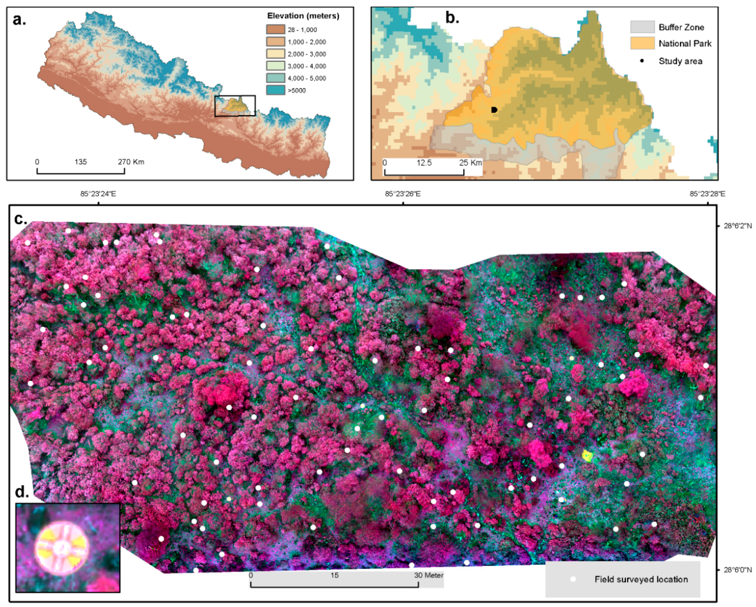
2.1. Study Area

The site for this study was located at 28.10° N, 85.3905° E and was inside Langtang National Park in central Nepal (Figure 1). Within the 0.81 ha study area the highest and lowest elevation recorded were 3791 m and 3766 m above mean sea level respectively and are part of the treeline ecotone. Abies spectabilis was a major treeline forming species while a tall shrub Rhododendron campanulatum was the spatially most dominant woody species followed by small shrubby species such as Rhododendron anthopogon and Berberis sp. Phenology of Rhododendron species appears to be highly sensitive to climate warming [43,44]. Therefore, these species have the potential to be used as indicator species for monitoring climate change impacts. Climate data from the nearest weather station showed that the average monthly total rainfall was highest in August (172.76 mm) and lowest in December (2.57 mm). Mean monthly temperature of the hottest (July) and coldest (December) month was 9.5 °C and −0.1 °C, respectively [45]. The understory was characterized by bare soil/rocky outcrops and non-photosynthetic vegetation (NPV) in the form of dry twigs and woody vegetation branches, possibly as a result of extraction of fuel wood by the local population and grazing by domesticated animals of nearby settlements.

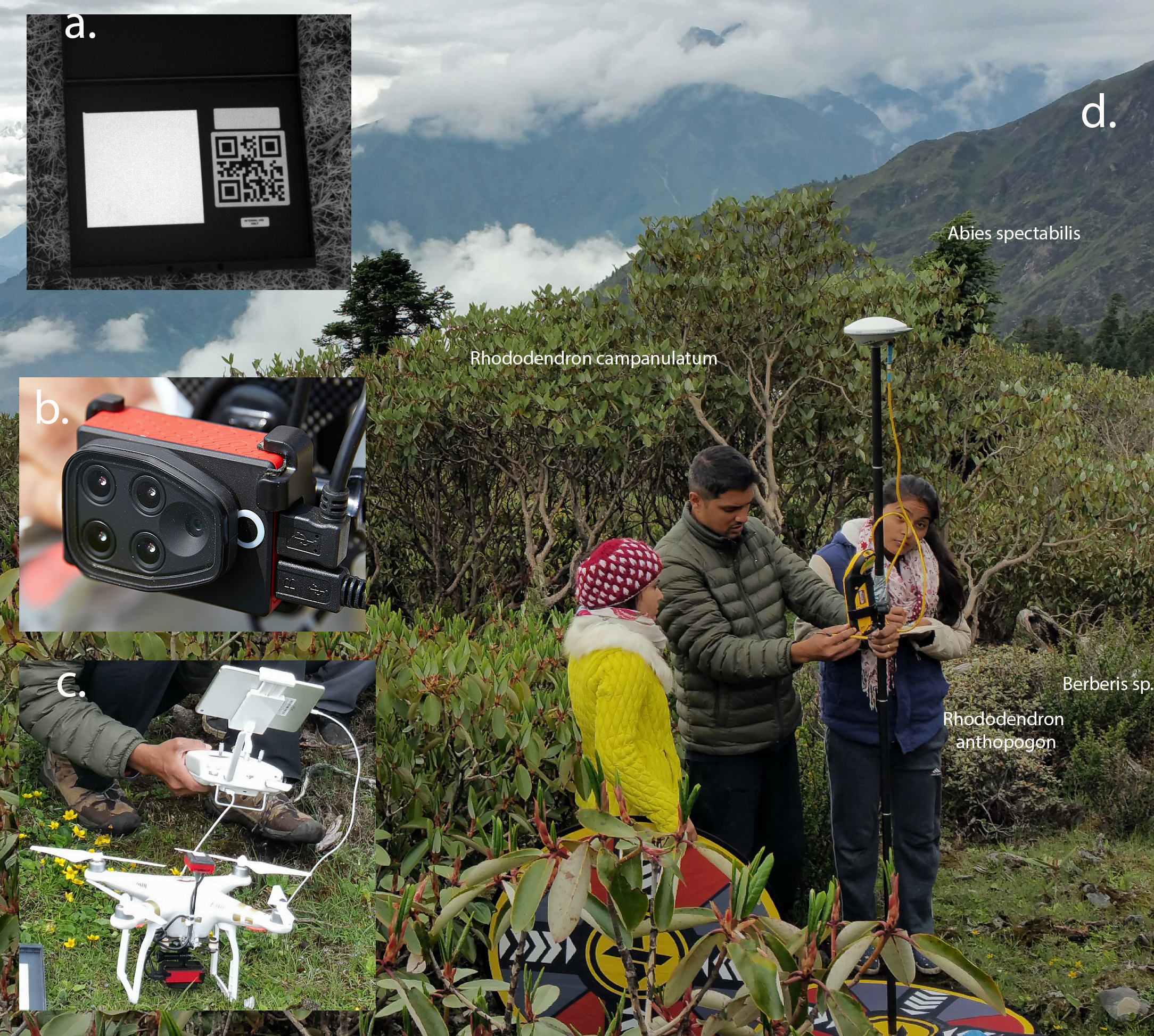
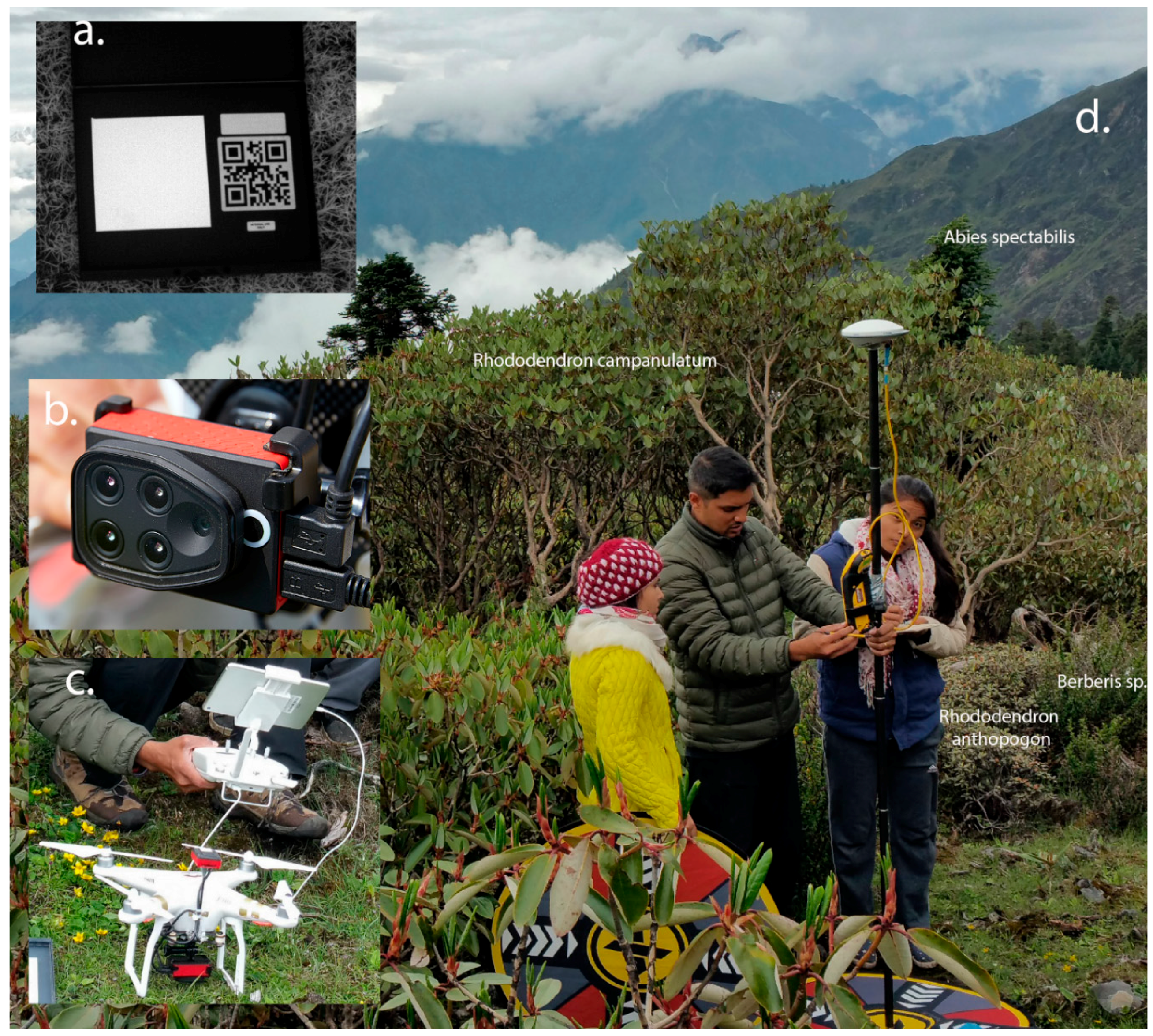
2.2. UAS Flight Missions and Ground Control Points

A consumer-grade Phantom-3 professional multirotor UAS (DJI Inc., Shenzhen, China) was used to carry a Parrot sequoia camera (MicaSense Inc., Seattle, WA, USA). Sequoia is a narrow band multi-spectral camera that acquires images in four wavelength bands at a resolution of 1.2 million pixels and has a global shutter rather than a rolling shutter (Table 1). The sequoia comes with a sunshine sensor which is mounted on top of the UAS (Figure 2c) and records irradiance in the same wavelength bands as the camera [42]. This information is utilized to calculate per-pixel reflectance values by accounting for the variability in ambient light conditions during the UAS mission [46]. UAS images were acquired on 16 June 2017 between 11 AM and noon under cloudy weather. To minimize the impact of terrain variability, the images were acquired in two flights missions each with separate launching location/height (Figure 1c). UAS data acquisition for both the missions were conducted in an automated manner using the Micasense Atlas Flight application with predefined parameters (i.e., flying height: 30 m above ground, velocity: 3 m/s and forward/side overlap of 80 percent). The two flights resulted in a total of 1240 geotagged images (310 images × 4 spectral bands) taken from near-nadir viewing geometry. Flights were conducted at stable illumination and fixed camera settings, aiming to acquire images at uniform conditions. Photos of a calibrated reflectance panel produced by the camera manufacturer (Figure 2a) were acquired immediately after the UAS flights. The average reflectance values of this panel for each waveband of the camera were utilized for calculating per-pixel reflectance.
Prior to the UAS flights, five Ground Control Points (GCPs) in the form of bull’s eye targets were deployed in the imaged area (example shown in Figure 1d and Figure 2). The three-dimensional co-ordinates (WGS 84, UTM zone 45N) were determined with a Trimble GeoXH 6000 handheld GPS connected to a Zephyer 2 antenna [47] mounted on a monopod (average positional accuracy < 0.5 m). GCPs were occupied for 15 min each (5 s interval) and received error correction from GAGAN, an operational satellite-based augmentation system (SBAS) [48]. As a post-processing step to reduce uncertainty in GCPs location; spatial mean was calculated from the 180 logged positions (over 15 min) to determine the accurate 3-D position of each GCP.

2.3. Field Survey and Identifying Vegetation Classes

Field data collection was conducted simultaneously with UAS flights. Within the study area, the location of 57 individual woody plants in total were recorded using the Trimble GeoXH 6000 system described earlier (2 min occupancy). Four major woody plant species identified in the study site were Abies spectabilis, Rhododendron campanulatum, Rhododendron anthopogon and Berberis sp. (Figure 2d). These four species along with herbaceous ground vegetation (grass, forbs, mosses, etc.) were photosynthetically active/green vegetation. Other cover types identified include bare soil/rocks and non-photosynthetic vegetation (NPV) were combined under and non-green vegetation class and sample locations representing them were also collected during field work.

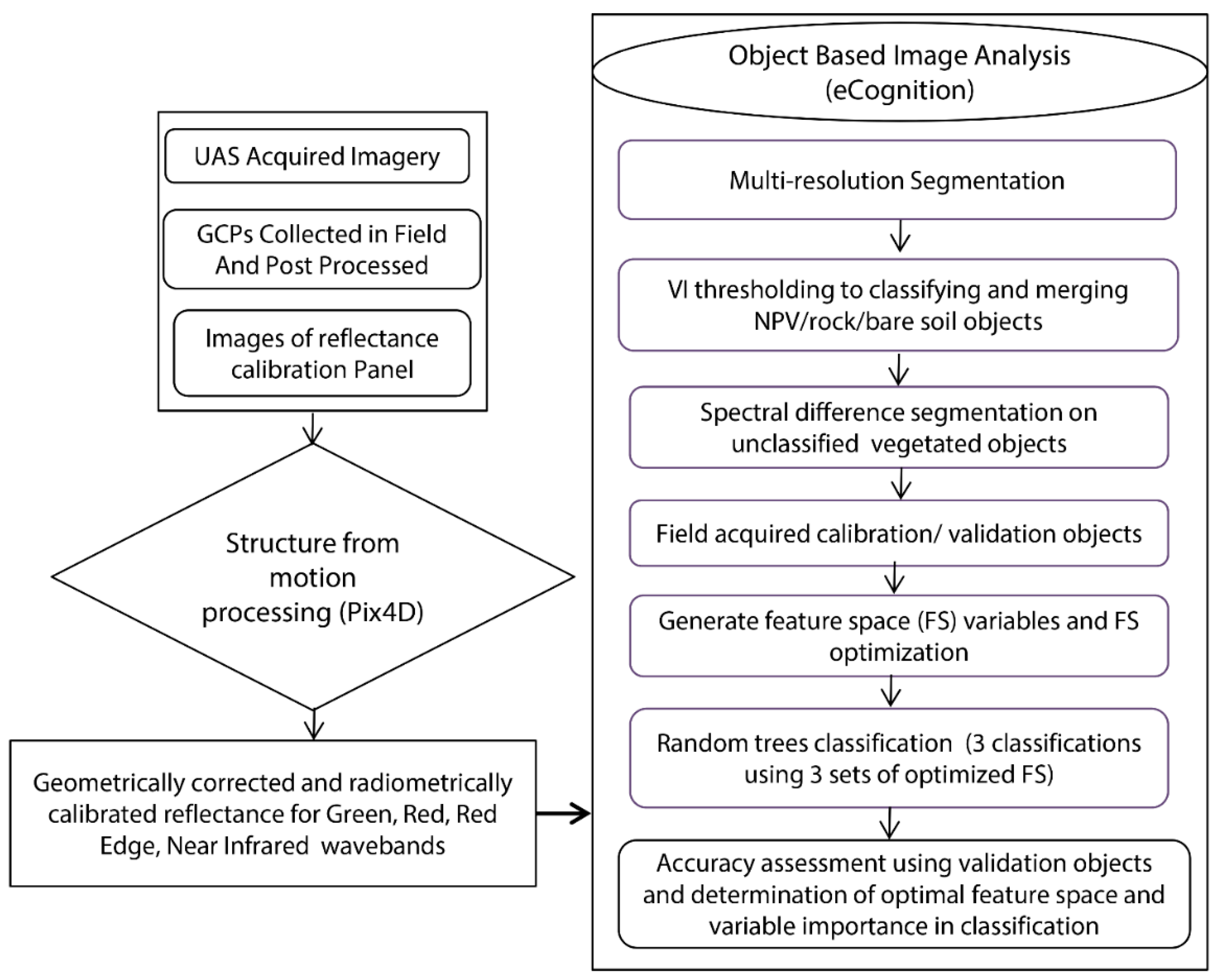
2.4. Image Processing

An overview of data collection and analysis workflow is shown in Figure 3. The UAS-derived images, GCP coordinates and images of the calibrated reflectance panel were brought into Pix4Dmapper Pro software (Lausanne, Switzerland) for processing via Structure-from-Motion (SfM). Following a standardized workflow, we selected the Ag Multispectral image processing template for processing [49]. The processing yielded an orthomosaic map, reflectance map and Normalized difference Vegetation Index (NDVI) for the study area with a ground sampling distance of 1.8 cm. Both orthomosaic and reflectance outputs are corrected for perspective error using a digital surface model (DSM). However, color balancing is applied on the orthomosaic to adjust the intensity of colors and produce a visually pleasing result. The reflectance bands are produced without any color balancing and the pixel values more accurately represent a target spectral reflectance [49]. Therefore, for detailed vegetation and cover type mapping this study utilized the reflectance bands.

2.5. Geographic Object Based Image Analysis (GEOBIA)

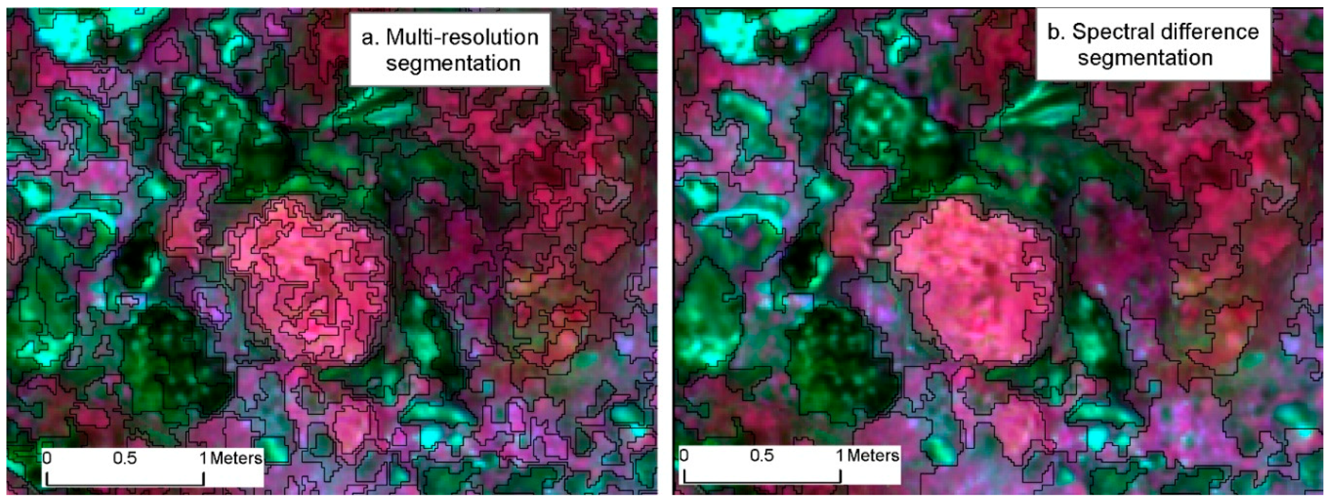
2.5.1. Segmentation and Level 1 Classification

The four reflectance bands and NDVI were stacked and multiplied by a scale factor of 10,000 and converted to a 16 bit unsigned integer to reduce data volume. A hierarchical GEOBIA was implemented into a eCognition Developer 9.2 (Trimble Inc., Sunnyvale, CA, USA) [50] that involved two steps: image segmentation and object classification. We first applied the multi-resolution segmentation (MRS) which generated objects by merging several pixels together based on relative homogeneity criteria [50]. This criteria is defined by setting values for the scale, shape/color and compactness/smoothness parameters. To generate smaller but spectrally pure objects, MRS was performed using a smaller scale factor (i.e., 50) and the red-edge (RE) band and the NDVI were given higher weights (1.5 and 2 respectively) to focus on photosynthetically active green vegetation. These values were deemed optimal after visually comparing results of several trial iterations. In the first classification, green vegetated objects were distinguished from other objects (bare soil/rock, non-photosynthetic vegetation) using NDVI thresholding where the optimal threshold was visually determined using the ‘feature view’ tool within eCognition Developer (Figure 4b).

2.5.2. Feature Space Selection and Level 2 Classification

Before the detailed classification of vegetated objects, a spectral difference segmentation (SDS) was performed only on the objects classified as green vegetation in level 1 classification. SDS merges neighboring objects if the difference in their spectral mean is below a given threshold (i.e., the objects are spectrally similar) [51]. Again, the optimal SDS parameters were determined by visually comparing results of several iterations. The resulting merged objects better represented the vegetation structure (e.g., a single tree stand represented by less than five objects after SDS compared to more than 20 objects before SDS) (Figure 4c). Training and validation objects for detailed classification at level 2 were selected by (i) intersecting surrounding image objects with specific sample for each class and (ii) including more objects in the neighborhood of field identified samples by visually confirming their cover type. This process resulted in the selection of a total of 386 sample objects, of which 240 (60%) were used for training and the remaining were used for accuracy assessment.
To determine the suitability of different classification features, this study performed three classifications at level 2 with the following three sets of features: only spectral features, spectral features + geometric/shape features and spectral features + geometric/shape features + textural features (Table 2). For each classification, the best features were selected using the Feature Space Optimization (FSO) and are shown in Table 3. The FSO tool calculates an optimum feature combination based on class samples and is available within eCognition. FSO evaluates the Euclidean distance in the feature space between the samples of all classes and selects a feature combination resulting in the best class separation distance, which is defined as the largest of the minimum distances between the least separable classes [50].
Level 2 classification was achieved using the random trees classifier (also called Random Forest) implemented within eCognition [52]. The random trees classifier builds multiple decision trees from bootstrap samples of the reference data. Each decision tree uses a random subset of training data and a random subset of input predictor variables. Roughly 2/3 of the data are sampled with replacement while 1/3 are withheld from tree construction (also called ‘out-of-the-bag’ or OOB samples). OOB samples are used to calculate the difference between predicted versus observed samples based on which error matrix is calculated.
Final class prediction is determined by majority voting based on the ensemble of trees. Random trees also calculate the measure of variable importance based on a random permutation of the input variables, and the effect of the permutation is quantified for each variable by the change in the OOB error [52]. Those variables important for separating classes show significant change in OOB error. Variable importance plot was generated and interpreted to determine the relative importance of feature variables. Classification accuracy was accessed using independent sample objects reserved for each class. Error matrices were calculated based on the number of objects per class without considering object size. Accuracy matrices reported include class-wise user’s (UA) and producer’s accuracy (PA), overall accuracy (OA) and kappa statistic (Table 4 and Table 5).

3. Results

Results of level 1 classification showed that about 65% of the mapped area was under green vegetation (Figure 5). The overall accuracy achieved for level 1 was 95.2% (Table 4), confirming that NDVI thresholding of objects by determining the optimal threshold value is simple yet an effective strategy for separating green vegetated objects from others (Figure 5a); this level of accuracy was observed by previous studies as well [54]. Further visual examination of level 1 classification results confirmed that some green vegetated objects with low vegetation density (dominated by Rhododendron anthopogon) had mean NDVI values below the threshold and resulted in false negative error (when classification erroneously predicted a low vegetation as non-vegetation object).
Based on the feature space selection method explained earlier, three optimized feature spaces were used that produced three classification outputs at level 2. Table 2 provides feature definitions and Table 3 lists all feature types that were used as candidate features and the numbering scheme explains if they were found to be optimal and used in final classification. Optimal features space using only spectral features consisted of 11 features. When both spectral and shape features were utilized, the optimal feature space consisted of 12 features (with only one shape feature) and when all three features (spectral + shape + texture) were utilized, the optimal feature space consisted of 16 features (11 spectral + 1 shape + 4 textural features). Results of level 2 classification using three sets of features show that the overall classification accuracy increased with the number and type of features used for classification. Highest overall accuracy (73%) and kappa (0.68) were obtained when all three feature types (spectral, shape, texture) were used. However, the accuracy with three feature types was not substantially higher compared to using just spectral features (accuracy of 70.77%) (Figure 5 and Table 5).
Per-class accuracy for level 2 results suggested that among green vegetation, Abies spectabilis was mapped with highest accuracy (100% UA), followed by Rhododendron campanulatum (85% UA), Rhododendron anthopogon (66% UA) and Berberis sp. (55% UA). Among non-green vegetated classes, bare soil/rock achieved 78% UA and non-photosynthetic vegetation was mapped at 69% UA. Spatial analysis show that Rhododendron campanulatum was spatially the most dominant cover type (31%) followed by Rhododendron anthopogon (25%) while Berberis sp. and Abies spectabilis were spatially least dominant (covering 3% and 2% area, respectively). Due to their larger spatial coverage, the inaccuracies in the mapping of the two Rhododendron species have higher ecological implications for monitoring treeline vegetation compared to others (e.g., Abies spectabilis) that are mapped at much higher accuracies.
Mapping accuracy was lower for Rhododendron anthopogon than Rhododendron campanulatum, and visual analysis showed that Rhododendron anthopogon was either misclassified as NPV or grass and bare soil was mistakenly classified as Rhododendron anthopogon. A possible explanation for this misclassification is the structural similarity between NPV and Rhododendron anthopogon (dwarf Rhododendron with dark green-to-brown small leaves and small shrubby structure). Although Rhododendron campanulatum was mapped with relatively higher accuracy, it was also misclassified as Rhododendron anthopogon. Visual analysis confirmed that this misclassification occurred in areas where Rhododendron campanulatum was immediately surrounded by dense Rhododendron anthopogon as the understory/below layer.
The best accuracy achieving classification for level 2 (Figure 5d) used 16 features. The variable importance plot (Figure 6) depicts 15 of these features in order of decreasing importance for discriminating vegetation at species level using multi-spectral UAS imagery. Mean NDVI at object level was the most important feature variable for level 2 classification. Furthermore, the presence of 13 spectral features among the top 15 features underscores the finding that spectral features alone provide an acceptable level of mapping accuracy. Adding shape and texture features improves the accuracy marginally. However it should be noted that classification using only spectral features was much faster (~6 min) compared to that using textural features (~50 min).

4. Discussion

The GEOBIA approach using multispectral UAS data has shown the potential for achieving species-level mapping for the Himalayan treeline ecotone. The exploratory work in finding the optimal segmentation approach (i.e., multi-resolution segmentation followed by spectral difference segmentation) and parameters (e.g., scale, shape and compactness criteria) helped in creating objects that were realistic in representing the spatial variability in the shape and size of the considered classes observed in the field (e.g., relatively larger and smooth canopy of Rhododendron campanulatum versus smaller size and compact shape of NPV and soil/rock surface).
The aim of species-level mapping was achieved with varying accuracy for different species. Certain classes could be mapped with better accuracy because of their morphological contrast. Broadleaved versus fine needle leaved species could be mapped with higher accuracies (e.g., Abies spectabilis and Berberis sp.) compared to structurally similar classes (e.g., Rhododendron anthopogon versus NPV).
When using spectral, spatial and textural features, we show that the spectral features contributed the most to a higher accuracy of species level mapping. Spectral features alone yielded ~70% accuracy because the species that were mapped were not only taxonomically different but also structurally different, allowing more accurate classification with spectral features. For example, Rhododendron campanulatum is much taller (mean height 1.5 m) than Rhododendron anthopogon (mean height 0.45 m), and has different architecture of branching and different types of leaves; Abies spectabilis is fine needle leaved, whereas Berberis sp. is broadleaved. Including texture and shape features improves the accuracy marginally, but substantially increases the computational time (nearly 20 times, i.e., from 5 min to about an hour). This can easily scale up to massive computational requirements for mapping over a larger area, as has been reported in previous studies [55]; importantly, inclusion of texture variables has a disproportional effect on computational requirements. It should be noted that the species diversity in our mapping space is not very high and it remains to be tested if variable importance and mapping accuracy will change if either species diversity increases or the study area becomes bigger.
This study opens up possibilities for future ecological research in the Himalaya, based on the invaluable capability of UAS as a tool for providing VHR data that can be useful for ecological monitoring in remote and inaccessible areas. Our results improve upon previous studies that utilized ecological niche models based on the probability of the occurrence approach to map the potential distribution of selected Himalayan species [56,57] instead of the direct classification approach.
As the UAS platform and sensors are becoming cheaper and more sophisticated, future studies should test the suitability of better cameras (e.g., Micasense RedEdge-M and Altum, Gamaya Hyperspectral) [58] as well as UAS platforms that fly for a longer duration to cover larger areas and have vertical take-off and landing capability for data collection mountainous terrain (e.g., FireFLY 6 Pro) [59]. Also, the effects of mission parameters (e.g., flying height, percent overlap) and changing terrain (especially in Himalaya with considerable slope) on resultant map quality needs to be tested to establish a framework for quality UAS imagery collection. Our experience from doing exploratory UAS missions in Langtang Himalaya with varying parameters indicates that the effect of slope and terrain can be minimized by diving the study area into more than one flight and keeping high overlap in images (>80%). However, even with these parameter settings, some edge area of the mission may lack sufficient overlap and would create artifacts which induce inaccuracies in classification output.
Given the potential of UAS data for ecological monitoring, the number of studies using GEOBIA for UAS images analysis is expected to increase. However, for achieving usable accuracies using GEOBIA substantial visual interpretation of objects is required to optimize segmentation parameters, and this can be a challenge in practical applications of GEOBIA over large areas. Therefore, among the possibilities for GEOBIA technique refinement, there is scope for developing algorithms that semi-automatically evaluate the outputs of multiple segmentations and are able to determine the most optimal segmentation parameters for users with limited human interpretation e.g., Reference [60].

5. Conclusions and Future Work

To the best of our knowledge, this study is the first ever application of multi-spectral UAS imagery for individual tree-level vegetation mapping in the Himalaya with the goal of identifying species. By testing the usefulness of features related to spectral, shape and texture attributes of vegetation in maximizing the accurate identification of species, we present the most optimal and parsimonious model for classification. The Himalayan vegetation, particularly at the treeline ecotone, exhibits a wide range in vegetation composition and structure and is increasingly responsive to environmental impacts and climate change. Understanding the ecological processes and community response requires data collection that should be unbiased and be able to generalize at the landscape level. However, that is a challenging task for the alpine Himalayan communities because of (1) the dramatically heterogeneous topography, environment and community structure on the mountain slopes requiring adequate sampling of vegetation in space, and, (2) the formidable challenges of staying longer in the study site for adequate sampling. We show that data collection using UAS images and field data in areas along the treeline ecotone in the Himalaya has the potential to increase time efficiency and lead to vegetation maps with acceptable accuracy at the species level. This study is, therefore, a step forward in developing valuable future mechanisms to monitor vegetation diversity for a highly understudied yet ecologically important biodiversity hotspots. The classification results of the UAS imagery depend on a number of factors including type of camera, spatial resolution of images, environmental conditions, appropriate pre-processing, vegetation physiognomy, and more. Therefore, future studies in the Himalaya would require adequate ground truthing for calibration and validation of models with semi-automated classification. With all that, a reasonably accurate model of classification of UAS imagery offers an efficient, cost effective method of vegetation species mapping that can be of value for extreme environments like the Himalaya. In summary, UAS and GEOBIA presents us with an unpresented opportunity of scaling up vegetation mapping by many orders of magnitude compared to traditional sampling. This immediately means a more generalizable understanding of ecological processes and responses can emerge out of UAS data.

Author Contributions

All authors contributed significantly to the manuscript. N.B.M. was responsible for original idea, collected field data and conducted data analysis. B.B.S. and D.K. contributed to field data collection and provided theoretical and conceptual inputs. J.R. and K.P.M. contributed to data analysis. N.B.M. drafted the manuscript and K.P.M. and B.B.S. contributed to manuscript revision.

Funding

N.B.M. was partially supported by a faculty research grant from the University of Wisconsin-La Crosse (UWL) and an equipment grant from the River Studies Center at UWL. J.R. was supported by the Research and Creativity Grant and the dean’s distinguished fellowship from the College of Science and Health at UWL.

Acknowledgments

The authors thank the Home Ministry, Civil Aviation Authority and the Department of National Parks and Wildlife Conservation of Nepal for giving the permission to collect UAS data; officials of Langtang National park for providing assistance and support. N.B.M. is thankful to the faculty of Central Department of Botany, Tribhuvan University for hosting him and providing assistance in securing UAS data collection permits. N.B.M. also gratefully acknowledges the help of students of Masters in Botany program at Tribhuvan University for logistical support and help with field data collection.

Conflicts of Interest

The authors declare no conflict of interest.

References

  1. Rapport, D.J. Evolution of indicators of ecosystem health. In Ecological Indicators; Springer: Berlin/Heidelberg, Germany, 1992; pp. 121–134. [Google Scholar]
  2. Elmqvist, T.; Folke, C.; Nyström, M.; Peterson, G.; Bengtsson, J.; Walker, B.; Norberg, J. Response diversity, ecosystem change, and resilience. Front. Ecol. Environ. 2003, 1, 488–494. [Google Scholar] [CrossRef] [Green Version]
  3. Fassnacht, F.E.; Latifi, H.; Stereńczak, K.; Modzelewska, A.; Lefsky, M.; Waser, L.T.; Straub, C.; Ghosh, A. Review of studies on tree species classification from remotely sensed data. Remote Sens. Environ. 2016, 186, 64–87. [Google Scholar] [CrossRef]
  4. Turner, W. Sensing biodiversity. Science 2014, 346, 301–302. [Google Scholar] [CrossRef] [PubMed]
  5. Kerr, J.T.; Ostrovsky, M. From space to species: Ecological applications for remote sensing. Trends Ecol. Evol. 2003, 18, 299–305. [Google Scholar] [CrossRef]
  6. Chawla, A.; Kumar, A.; Lal, B.; Singh, R.; Thukral, A.K. Ecological Characterization of High Altitude Himalayan Landscapes in the Upper Satluj River Watershed, Kinnaur, Himachal Pradesh, India. J. Indian Soc. Remote Sens. 2012, 40, 519–539. [Google Scholar] [CrossRef]
  7. Munsi, M.; Areendran, G.; Ghosh, A.; Joshi, P. Landscape characterisation of the forests of Himalayan foothills. J. Indian Soc. Remote Sens. 2010, 38, 441–452. [Google Scholar] [CrossRef]
  8. Mishra, N.B.; Mainali, K.P. Greening and browning of the Himalaya: Spatial patterns and the role of climatic change and human drivers. Sci. Total Environ. 2017, 587, 326–339. [Google Scholar] [CrossRef] [PubMed]
  9. Lele, N.; Joshi, P. Analyzing deforestation rates, spatial forest cover changes and identifying critical areas of forest cover changes in North-East India during 1972–1999. Environ. Monit. Assess. 2009, 156, 159. [Google Scholar] [CrossRef] [PubMed]
  10. Qamer, F.M.; Shehzad, K.; Abbas, S.; Murthy, M.; Xi, C.; Gilani, H.; Bajracharya, B. Mapping deforestation and forest degradation patterns in western Himalaya, Pakistan. Remote Sens. 2016, 8, 385. [Google Scholar] [CrossRef]
  11. Krishnaswamy, J.; John, R.; Joseph, S. Consistent response of vegetation dynamics to recent climate change in tropical mountain regions. Glob. Chang. Biol. 2014, 20, 203–215. [Google Scholar] [CrossRef] [PubMed]
  12. Chakraborty, A.; Sachdeva, K.; Joshi, P. Mapping long-term land use and land cover change in the central Himalayan region using a tree-based ensemble classification approach. Appl. Geogr. 2016, 74, 136–150. [Google Scholar] [CrossRef]
  13. Gilani, H.; Shrestha, H.L.; Murthy, M.; Phuntso, P.; Pradhan, S.; Bajracharya, B.; Shrestha, B. Decadal land cover change dynamics in Bhutan. J. Environ. Manag. 2015, 148, 91–100. [Google Scholar] [CrossRef] [PubMed]
  14. Uddin, K.; Shrestha, H.L.; Murthy, M.; Bajracharya, B.; Shrestha, B.; Gilani, H.; Pradhan, S.; Dangol, B. Development of 2010 national land cover database for the Nepal. J. Environ. Manag. 2015, 148, 82–90. [Google Scholar] [CrossRef] [PubMed]
  15. Niklas, K.J.; Midgley, J.J.; Rand, R.H. Tree size frequency distributions, plant density, age and community disturbance. Ecol. Lett. 2003, 6, 405–411. [Google Scholar] [CrossRef]
  16. Sundriyal, R.; Sharma, E.; Rai, L.; Rai, S. Tree structure, regeneration and woody biomass removal in a sub-tropical forest of Mamlay watershed in the Sikkim Himalaya. Vegetatio 1994, 113, 53–63. [Google Scholar] [CrossRef]
  17. Gairola, S.; Sharma, C.; Ghildiyal, S.; Suyal, S. Regeneration dynamics of dominant tree species along an altitudinal gradient in moist temperate valley slopes of the Garhwal Himalaya. J. For. Res. 2012, 23, 53–63. [Google Scholar] [CrossRef]
  18. Gairola, S.; Procheş, Ş.; Rocchini, D. High-resolution satellite remote sensing: A new frontier for biodiversity exploration in Indian Himalayan forests. Int. J. Remote Sens. 2013, 34, 2006–2022. [Google Scholar] [CrossRef]
  19. Li, D.; Ke, Y.; Gong, H.; Li, X. Object-based urban tree species classification using bi-temporal WorldView-2 and WorldView-3 images. Remote Sens. 2015, 7, 16917–16937. [Google Scholar] [CrossRef]
  20. Ghosh, A.; Joshi, P. A comparison of selected classification algorithms for mapping bamboo patches in lower Gangetic plains using very high resolution WorldView 2 imagery. Int. J. Appl. Earth Observ. Geoinf. 2014, 26, 298–311. [Google Scholar] [CrossRef]
  21. Yan, J.; Zhou, W.; Han, L.; Qian, Y. Mapping vegetation functional types in urban areas with WorldView-2 imagery: Integrating object-based classification with phenology. Urban For. Urban Green. 2018, 31, 230–240. [Google Scholar] [CrossRef]
  22. Van Deventer, H.; Cho, M.; Mutanga, O. Improving the classification of six evergreen subtropical tree species with multi-season data from leaf spectra simulated to WorldView-2 and RapidEye. Int. J. Remote Sens. 2017, 38, 4804–4830. [Google Scholar] [CrossRef]
  23. Shi, P.; Wu, N. The timberline ecotone in the Himalayan region: An ecological review. In High-Altitude Rangelands and Their Interfaces in the Hindu Kush Himalayas; International Centre for Integrated Mountain Development: Patan, Nepal, 2013; Volume 108. [Google Scholar]
  24. Liang, E.; Wang, Y.; Piao, S.; Lu, X.; Camarero, J.J.; Zhu, H.; Zhu, L.; Ellison, A.M.; Ciais, P.; Peñuelas, J. Species interactions slow warming-induced upward shifts of treelines on the Tibetan Plateau. Proc. Natl. Acad. Sci. USA 2016, 113, 4380–4385. [Google Scholar] [CrossRef] [PubMed]
  25. Schickhoff, U.; Bobrowski, M.; Böhner, J.; Bürzle, B.; Chaudhary, R.; Gerlitz, L.; Heyken, H.; Lange, J.; Müller, M.; Scholten, T. Do Himalayan treelines respond to recent climate change? An evaluation of sensitivity indicators. Earth Syst. Dyn. 2015, 6. [Google Scholar] [CrossRef]
  26. Chhetri, P.K. Use of High Resolution DigitalGlobe Satellite Imagery to Map the Alpine Treeline Ecotone of the Nepal Himalaya. Digit. Glob Funadation 2015. [Google Scholar]
  27. Körner, C. Plant adaptation to cold climates. F1000Research 2016, 5. [Google Scholar] [CrossRef] [PubMed]
  28. Asner, G.P.; Knapp, D.E.; Boardman, J.; Green, R.O.; Kennedy-Bowdoin, T.; Eastwood, M.; Martin, R.E.; Anderson, C.; Field, C.B. Carnegie Airborne Observatory-2: Increasing science data dimensionality via high-fidelity multi-sensor fusion. Remote Sens. Environ. 2012, 124, 454–465. [Google Scholar] [CrossRef]
  29. Ghosh, A.; Fassnacht, F.E.; Joshi, P.; Koch, B. A framework for mapping tree species combining hyperspectral and LiDAR data: Role of selected classifiers and sensor across three spatial scales. Int. J. Appl. Earth Observ. Geoinf. 2014, 26, 49–63. [Google Scholar] [CrossRef]
  30. Näsi, R.; Honkavaara, E.; Lyytikäinen-Saarenmaa, P.; Blomqvist, M.; Litkey, P.; Hakala, T.; Viljanen, N.; Kantola, T.; Tanhuanpää, T.; Holopainen, M. Using UAV-based photogrammetry and hyperspectral imaging for mapping bark beetle damage at tree-level. Remote Sens. 2015, 7, 15467–15493. [Google Scholar] [CrossRef]
  31. Capolupo, A.; Kooistra, L.; Berendonk, C.; Boccia, L.; Suomalainen, J. Estimating plant traits of grasslands from UAV-acquired hyperspectral images: A comparison of statistical approaches. ISPRS Int. J. Geo-Inf. 2015, 4, 2792–2820. [Google Scholar] [CrossRef]
  32. Chen, G.; Weng, Q.; Hay, G.J.; He, Y. Geographic Object-based Image Analysis (GEOBIA): Emerging trends and future opportunities. GISci. Remote Sens. 2018, 55, 159–182. [Google Scholar] [CrossRef]
  33. Blaschke, T.; Hay, G.J.; Kelly, M.; Lang, S.; Hofmann, P.; Addink, E.; Feitosa, R.Q.; Van der Meer, F.; Van der Werff, H.; Van Coillie, F. Geographic object-based image analysis–towards a new paradigm. ISPRS J. Photogramm. Remote Sens. 2014, 87, 180–191. [Google Scholar] [CrossRef] [PubMed]
  34. Mishra, N.B.; Crews, K.A. Mapping vegetation morphology types in a dry savanna ecosystem: Integrating hierarchical object-based image analysis with Random Forest. Int. J. Remote Sens. 2014, 35, 1175–1198. [Google Scholar] [CrossRef]
  35. Blaschke, T. Object based image analysis for remote sensing. ISPRS J. Photogramm. Remote Sens. 2010, 65, 2–16. [Google Scholar] [CrossRef]
  36. Franklin, S.E.; Ahmed, O.S. Deciduous tree species classification using object-based analysis and machine learning with unmanned aerial vehicle multispectral data. Int. J. Remote Sens. 2017. [Google Scholar] [CrossRef]
  37. Komárek, J.; Klouček, T.; Prošek, J. The potential of Unmanned Aerial Systems: A tool towards precision classification of hard-to-distinguish vegetation types? Int. J. Appl. Earth Observ. Geoinf. 2018, 71, 9–19. [Google Scholar] [CrossRef]
  38. Oldeland, J.; Große-Stoltenberg, A.; Naftal, L.; Strohbach, B. The potential of UAV derived image features for discriminating savannah tree species. In The Roles of Remote Sensing in Nature Conservation; Springer: Berlin/Heidelberg, Germany, 2017; pp. 183–201. [Google Scholar]
  39. Lu, B.; He, Y. Species classification using Unmanned Aerial Vehicle (UAV)-acquired high spatial resolution imagery in a heterogeneous grassland. ISPRS J. Photogramm. Remote Sens. 2017, 128, 73–85. [Google Scholar] [CrossRef]
  40. Kachamba, D.J.; Ørka, H.O.; Næsset, E.; Eid, T.; Gobakken, T. Influence of plot size on efficiency of biomass estimates in inventories of dry tropical forests assisted by photogrammetric data from an unmanned aircraft system. Remote Sens. 2017, 9, 610. [Google Scholar] [CrossRef]
  41. Bhardwaj, A.; Sam, L.; Martín-Torres, F.J.; Kumar, R. UAVs as remote sensing platform in glaciology: Present applications and future prospects. Remote Sens. Environ. 2016, 175, 196–204. [Google Scholar] [CrossRef]
  42. MicaSense, Inc. Available online: https://www.micasense.com/parrotsequoia/ (accessed on 11 October 2017).
  43. Gaira, K.S.; Rawal, R.S.; Rawat, B.; Bhatt, I.D. Impact of climate change on the flowering of Rhododendron arboreum in central Himalaya, India. Curr. Sci. 2014, 106, 1735–1738. [Google Scholar]
  44. Hart, R.; Salick, J.; Ranjitkar, S.; Xu, J. Herbarium specimens show contrasting phenological responses to Himalayan climate. Proc. Natl. Acad. Sci. USA 2014, 201403376. [Google Scholar] [CrossRef] [PubMed]
  45. Gaire, N.; Dhakal, Y.; Lekhak, H.; Bhuju, D.; Shah, S. Vegetation dynamics in treeline ecotone of Langtang National Park, Central Nepal. Nepal J. Sci. Technol. 2010, 11, 107–114. [Google Scholar] [CrossRef]
  46. Assmann, J.J.; Kerby, J.T.; Cunliffe, A.M.; Myers-Smith, I.H. Vegetation monitoring using multispectral sensors-best practices and lessons learned from high latitudes. bioRxiv 2018, 334730. [Google Scholar] [CrossRef]
  47. Trimble. Trimble GeoXH 6000 User Guide. Available online: https://tinyurl.com/ybkgjj33 (accessed on 23 January 2018).
  48. Rao, K. GAGAN-The Indian satellite based augmentation system. India J. Raio Space Phys. 2007, 36, 293–304. [Google Scholar]
  49. Pix4D. Pix4D Mapper User Manual. Available online: https://support.pix4d.com/hc/en-us/articles/204272989-Offline-Getting-Started-and-Manual-pdf- (accessed on 2 October 2017).
  50. eCognition Developer, T. 9.0 User Guide; Trimble Germany GmbH: Munich, Germany, 2014.
  51. Mikeš, S.; Haindl, M.; Scarpa, G.; Gaetano, R. Benchmarking of remote sensing segmentation methods. IEEE J. Sel. Top. Appl. Earth Observ. Remote Sens. 2015, 8, 2240–2248. [Google Scholar] [CrossRef]
  52. Breiman, L. Random forests. Mach. Learn. 2001, 45, 5–32. [Google Scholar] [CrossRef]
  53. Haralick, R.M.; Shanmugam, K.; Dinstein, I.H. Textural features for image classification. IEEE Trans. Syst. Man Cybern. 1973, 3, 610–621. [Google Scholar] [CrossRef]
  54. Laliberte, A.; Browning, D.; Herrick, J.; Gronemeyer, P. Hierarchical object-based classification of ultra-high-resolution digital mapping camera (DMC) imagery for rangeland mapping and assessment. J. Spat. Sci. 2010, 55, 101–115. [Google Scholar] [CrossRef]
  55. Mishra, N.B. Characterizing Ecosystem Structural and Functional Properties in the Central Kalahari Using Multi-Scale Remote Sensing. Ph.D. Thesis, The University of Texas at Austin, Austin, TX, USA, 2014. [Google Scholar]
  56. Ranjitkar, S.; Kindt, R.; Sujakhu, N.M.; Hart, R.; Guo, W.; Yang, X.; Shrestha, K.K.; Xu, J.; Luedeling, E. Separation of the bioclimatic spaces of Himalayan tree rhododendron species predicted by ensemble suitability models. Glob. Ecol. Conserv. 2014, 1, 2–12. [Google Scholar] [CrossRef]
  57. Kumar, P. Assessment of impact of climate change on Rhododendrons in Sikkim Himalayas using Maxent modelling: Limitations and challenges. Biodivers. Conserv. 2012, 21, 1251–1266. [Google Scholar] [CrossRef]
  58. MicaSense, Inc. RedEdge M User Manual. Available online: https://support.micasense.com/hc/en-us/articles/115003537673-RedEdge-M-User-Manual-PDF- (accessed on 14 February 2018).
  59. BirdsEyeView. FifeFly 6 Pro User Manaul. 2017. Available online: https://tinyurl.com/y8qpsgso (accessed on 28 May 2018).
  60. Gao, H.; Tang, Y.; Jing, L.; Li, H.; Ding, H. A Novel Unsupervised Segmentation Quality Evaluation Method for Remote Sensing Images. Sensors 2017, 17, 2427. [Google Scholar] [CrossRef] [PubMed]
Figure 1. (a) Study area location in Nepal Himalaya showing elevation range; (b) location of study area within Langtang National Park, Nepal; (c) field vegetation sampling locations overlaid on multispectral orthomosaic for the study area created from UAS imagery; and (d) ground control point.
Ijgi 07 00445 g001
Figure 2. (a) Calibration panel used for estimating surface reflectance; (b) Sequoia camera that acquires images at fixed wavelengths including red-edge and near-infrared; (c) the entire UAS setup with remote and tablet used for mission planning; and (d) setting up ground control points (GCPs) prior to UAS mission in the treeline ecotone in Langtang national park (image date June, 2016). Also labeled are the woody species mapped in this study.
Ijgi 07 00445 g002
Figure 3. Workflow of data collection, pre-processing and analysis to produce a species classification map.
Ijgi 07 00445 g003
Figure 4. Results of the segmentation method used in this study (background image band combination: Blue: green band, Green: red band and Red: red edge band).
Ijgi 07 00445 g004
Figure 5. GEOBIA classification outputs for level 1 and level 2 classification.
Ijgi 07 00445 g005
Figure 6. Variable importance of various feature used for random forest classification. Only the top 15 variables are shown.
Ijgi 07 00445 g006
Table 1. Camera and flights parameters used in this study.
Camera PropertiesValues
Wavelength bands/central wavelengthGreen (550 nm), Red (660 nm),
Red Edge (735 nm), NIR (790 nm)
Focal length4.0 mm
Image resolution1280 × 960 pixels
Imager size4.8 mm × 3.6 mm
Horizontal FOV61.9°
Vertical FOV48.5°
Radiometric resolution/format12 bit/TIFF
Flying height30 m (above ground level)
Resulting GSD1.8 cm
Study area considered in 2 flights0.81 ha
Table 2. Definition of the selected features that were used in image classification.
FeatureDescription
Mean layer valueThe mean value represents the mean brightness of an image object within a single band
Standard deviationThe standard deviation of all pixels which form an image object within a band
Spectral indicesNormalized Difference Vegetation Index (NDVI) calculated as (NIR-red)/(NIR + red); Green Index (GI) calculated as (NIR-green)/(NIR + green); Red Edge Index (REI) calculated as (NIR-red edge)/(NIR + red edge)
Maximum differenceMinimum mean value of an object subtracted from its maximum value. The means of all bands belonging to an object are compared with each other and the result is divided by the brightness [50].
ShapeBorder index: Describes how jagged an image object is, the more jagged, the higher its border index. Shape Index: a measure of overall shape complexity and it is calculated from the border length feature of the image object divided by four times the square root of its area [50].
Texture after HaralickGLCM (grey level co-occurrence matrix) calculated after Haralick, Shanmugam, and Dinstein [53] describes how different combinations of pixel values occur within an object; used features (using the mean of all layers).
Table 3. Selected optimal feature used for classification; 1 optimal feature space with only spectral features, 1,2 optimal feature space with spectral + shape features and 1,2,3 optimal feature space with spectral + shape+ textural features.
Spectral ShapeTexture
Mean Green 1,2AsymmetryGLCM homogeneity 3
Mean Red 1,2,3Border Index 2GLCM contrast
Mean Red edge 3CompactnessGLCM dissimilarity 3
Mean NIR 1,2,3Rectangular fitGLCM entropy 3
Standard deviation Green 1,2,3RoundnessGLCM angular 2nd moment
Standard deviation Red 1,2,3Shape Index 2,3GLCM mean 3
Standard deviation Red edgeDensityGLCM Standard deviation
Standard deviation NIR 1,2,3 GLCM correlation
Maximum difference 2,3
Mean NDVI 1,2,3
Mean GI
Mean REI 1,3
Standard deviation NDVI 1,2,3
Standard deviation GI 1
Standard deviation REI 1,2,3
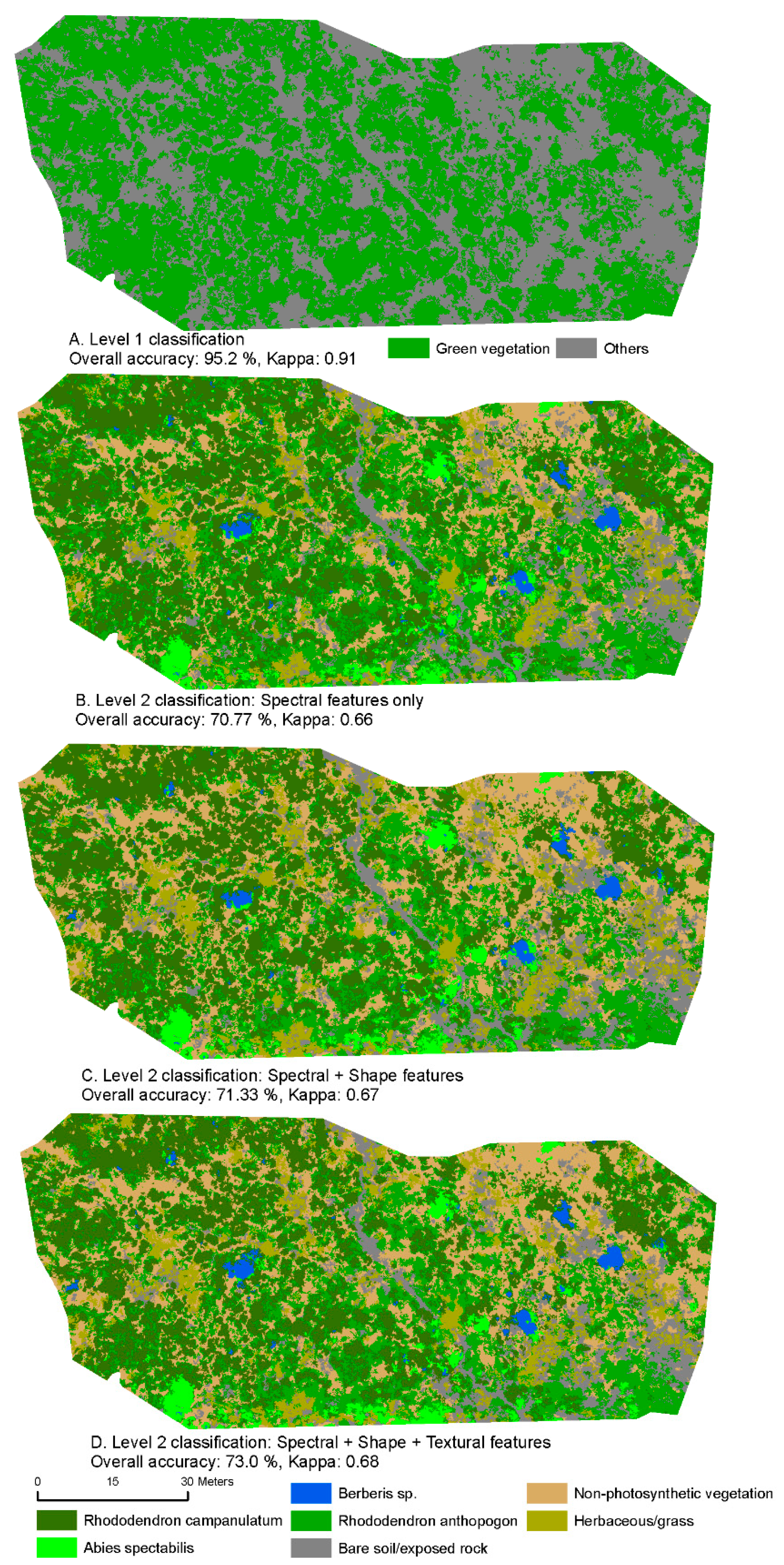
Table 4. Confusion matrix for level 1 classification achieved using NDVI thresholding.
Cover TypeGreen VegetationOthersTotalProducer’s Accuracy
(1-Omission Error)
Green vegetation9539897%
Others4444892%
Total9947146-
User’s accuracy
(1-comission error)
96%94%-95.2%
Table 5. Confusion matrix for level 2 classification achieved using random trees and all features (spectral + shape + texture).
Cover TypeRhodo Camp.Rhodo Antho.Berberis sp.Abies Spec.GrassNPVBare Soil/RockTotalProducer’s Accuracy
Rhodo camp.418100105180%
Rhodo antha.532206525257%
Berberis sp.1050120955%
Abies spec.1006010875%
Grass021015302171%
NPV030012933680%
Bare soil/rock030011182378%
Total484896244223146-
User’s accuracy85%66%55%100%62%69%78%-73%

