1. Introduction
Soil erosion in German vineyard plantations is a major concern to farmers and policymakers, particularly where slopes are steep, and soil erosion investigation started nearly 50 years ago [
1]. However, soil erosion mitigation measures are scarce largely because they are very costly, tedious to implement on the steep slopes, and there is a lack of awareness by some farmers and farm managers. In addition, the high stone contents in German vineyards contribute to a high variability of the hydrological processes, making it very difficult to implement soil erosion control strategies [
2]. Regardless, some strategies of soil erosion protection, such as the use of grass cover [
3], shrub covers [
4] or straw mulches [
5], have been implemented with successful results in numerous Mediterranean areas. These could also be applied in the Ruwer-Mosel valley in Germany, but it seems some farmers are not convinced of the value of such erosion control measures. Thus, there is a need to develop an accurate, visually attractive, and user-friendly survey method to highlight the rate of soil loss through erosion that could help to increase stakeholders´ awareness and encourage their participation in erosion control and mitigation.
Several methods, involving rainfall simulations [
6], modelling techniques [
7] and Gerlach troughs or pins in erosion plots [
8,
9] have been conducted in vineyards to quantify soil erosion rates. However, rainfall simulations are able to quantify initial soil erosion processes but for only a few controlled events and at the pedon scale [
9], which in vineyards may not be representative enough due to the high variability of natural rainfall in some cases. Open or enclosed erosion plots, Gerlach troughs, and pins need several years of monitoring (>3 or 5 years) before soil loss can be estimated accurately because of the high climate and pedological variability [
10,
11]. Moreover, these methods are characterised as being invasive because external objects have to be installed into the soil.
The stock unearthing method (SUM), a non-invasive technique, could be considered as an appropriate method for measuring long-term soil erosion in vineyards [
12]. It uses the elevation difference between the current soil surface level and the graft union (which serves as a passive bioindicator or botanical benchmark) to estimate total soil mobilisation rates [
13,
14]. Recently, improvements (ISUM—improved stock unearthing method) were done by taking measurements at the graft union as well as several locations within the inter-row areas of opposite pair vines. ISUM better detects linear soil erosion features such as rills and ephemeral gullies [
15]. However, a shortcoming of ISUM is that there are gaps in the order of centimetres within the cross-sectional areas that are not captured. Therefore, the highest possible accuracy for soil erosion estimations cannot be reached using only the SUM or ISUM.
In order to fill the missing data gaps, a structure-from-motion (SfM) photogrammetry technique could be employed in combination with SUM to improve erosion measurement accuracy in vineyards. SfM allows calculation of a continuous three-dimensional model of the soil surface by means of photogrammetric approaches [
16,
17]. It is widely used in environmental sciences and, specifically, in soil erosion surveys [
18,
19]. SfM allows computation of three-dimensional models using two-dimensional photos taken from different angles [
20,
21]. If the preparatory work is properly conducted, the derived models are of a striking accuracy due to the use of high-resolution photographs in combination with carefully selected points of view and exposure conditions. Notable examples using SfM to survey transient surface changes can be found in References [
20,
21].
Different devices, such as mobile phones and hand-held cameras [
22], have been applied to conduct SfM measurements but the determination of the initial soil surface level (t
0) using environmental markers, or qualitative observations, introduces errors in the measurements, leading to inaccurate soil erosion estimation. Thus, SfM could be used to enhance the spatial resolution of SUM, and in return, the reference level of SfM could be set to the position of the initial soil surface level at the time of plantation commencement provided by SUM. The main aim of this research was to combine the methodologies of the stock unearthing and SfM to map the current soil surface level to improve the accuracy of the estimate of soil mobilisation rates in vineyards. This methodological research could present an improved, low-tech and low-cost method to assess the long-term soil erosion processes in vineyards, with a higher accuracy compared with ISUM. We consider that conducting more accurate and visually-friendly soil erosion surveys would help us to understand soil erosion processes in sloping vineyards. Moreover, we strongly agree that it would increase stakeholders´ awareness of the need to guard their vineyards against land degradation processes.
2. Materials and Methods
2.1. Study Area
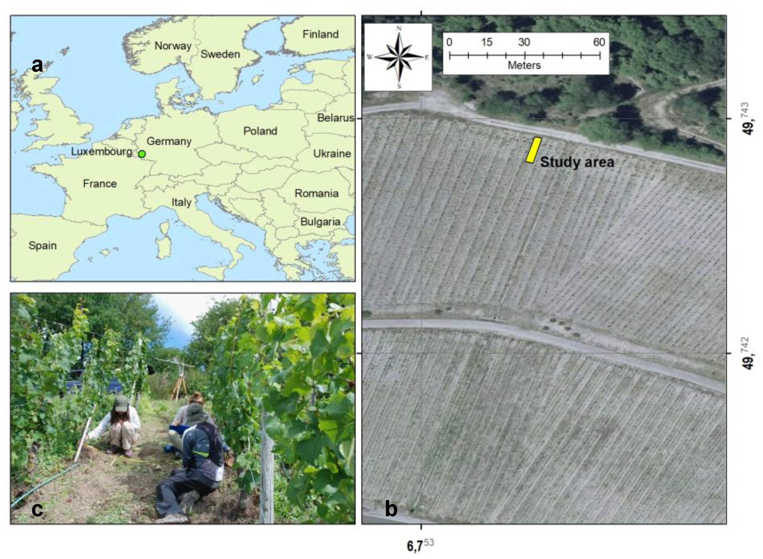
The study area (latitude 49.7418 N; longitude 6.7524 E) shown in
Figure 1 is located on the sloping vineyards of Waldrach, a small village in the Ruwer Valley, Rhineland-Palatinate, Germany. The geology belongs to the Rhenish metamorphic unit, characterised by the Hunsrück Slate, a Lower Devonian lithostratigraphic unit. The lithology is, therefore, characterised by Devonian greywackes, slates, partially quartzites, and Pleistocene silts deposited near the Ruwer River, an affluent of the Mosel River. The Riesling is the grape variety of this vineyard which is a conventionally managed 40-year-old plantation. The vines are regular vertically-trellised in the direction of dip of slope length varying between 60 m and 75 m.
The paired-vine rows are separated by 1.7 m and the inter-vine distance on the same row is 0.9 m. Slope angles vary from 15 to 30° with a general convex morphology and the altitude ranges between 190 and 270 m a.s.l. Grass cover and trees can be observed downslope near the vineyard and the agricultural roads.
The soils are classified as leptic-humic Regosols [
23]. The horizons are characterised by a stone content of 37.9%. Soil particle analysis indicated 64.7% silt, 26% sand and 9.3% clay. On average the field capacity (FC) of the soil is 30% and the wilting point (WP) is 12.3%. Other properties of the soil are: total organic carbon (TOC) is 7.9% along with a soil profile of about 25 cm depth, carbonate content (CaCO
3) < 1%, electrical conductivity (EC) is 0.35 dS m
−1, pH
water is 7.2, and potassium chloride (KCl) is 6.4%. Therefore, no soil acidification trends are noted. More information about the soil properties can be found in Reference [
2].
The average annual rainfall is 765 mm and the maximum amounts occur during the summer months, mostly during thunderstorms. The mean annual temperature is around 9°C, with maximum values in June, July and August (16.2–17.6 °C) and minimum values in January and December (1.5–2.3 °C).
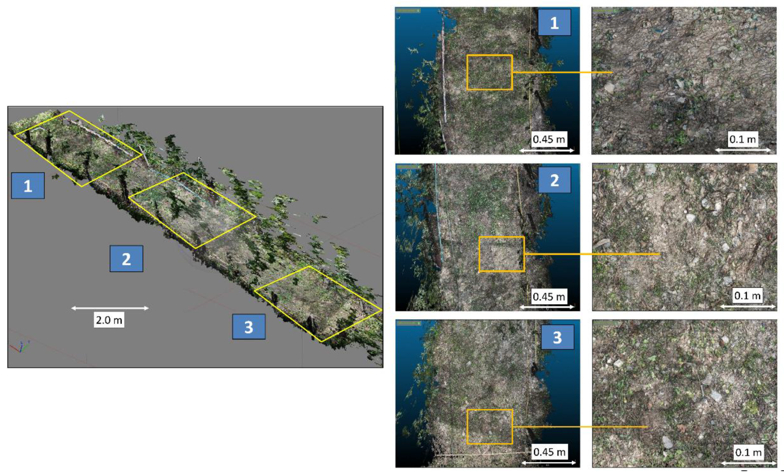
The yearly soil management is as follows: (i) a mechanical soil tillage (20 cm depth); (ii) removal of grass cover in the inter-row (with maximum height of 20 cm) and in the rows (between 10 cm and 35 cm height); (iii) a utilisation of a slate rock fragment cover to keep the soil temperature stable; and (vi) the use of pesticides and herbicides during spring and summer to eliminate weeds. Rills and ephemeral gullies (caused by wheel tracks and footpaths) located in the embankments and inter-row areas can be noted in
Figure 2.
2.2. The Stock Unearthing Method (SUM) and Its Improvement (ISUM, Improved Stock Unearthing Method)
The main aim of these soil erosion surveys in vineyards is to estimate the long-term soil mobilisation by observing the distance between the marks on the graft union and the current soil surface level (SUM), and extra measurements taken in the inter-row areas (ISUM) [
16].
The necessity to graft vine stocks occurred during the period of 1860–1920 because of the
Phylloxera crisis in which a large part of the commercial grapevines around Europe was infected by a pest (
Daktulosphaira vitifoliae), originally native to eastern North America [
24,
25]. The solution was to graft the vines onto an American vine stock, which now shows an unearthing or buried signal [
12,
14]. The vine graft unions are a clear signal of the initial height above the soil surface at the time of planting because the original vine stock does not grow vertically [
26].
SUM (stock unearthing method) and ISUM (improved stock unearthing method) are well-established methods used for case studies such as the differentiation of soil mobilisation in vineyards with different ages and parent materials [
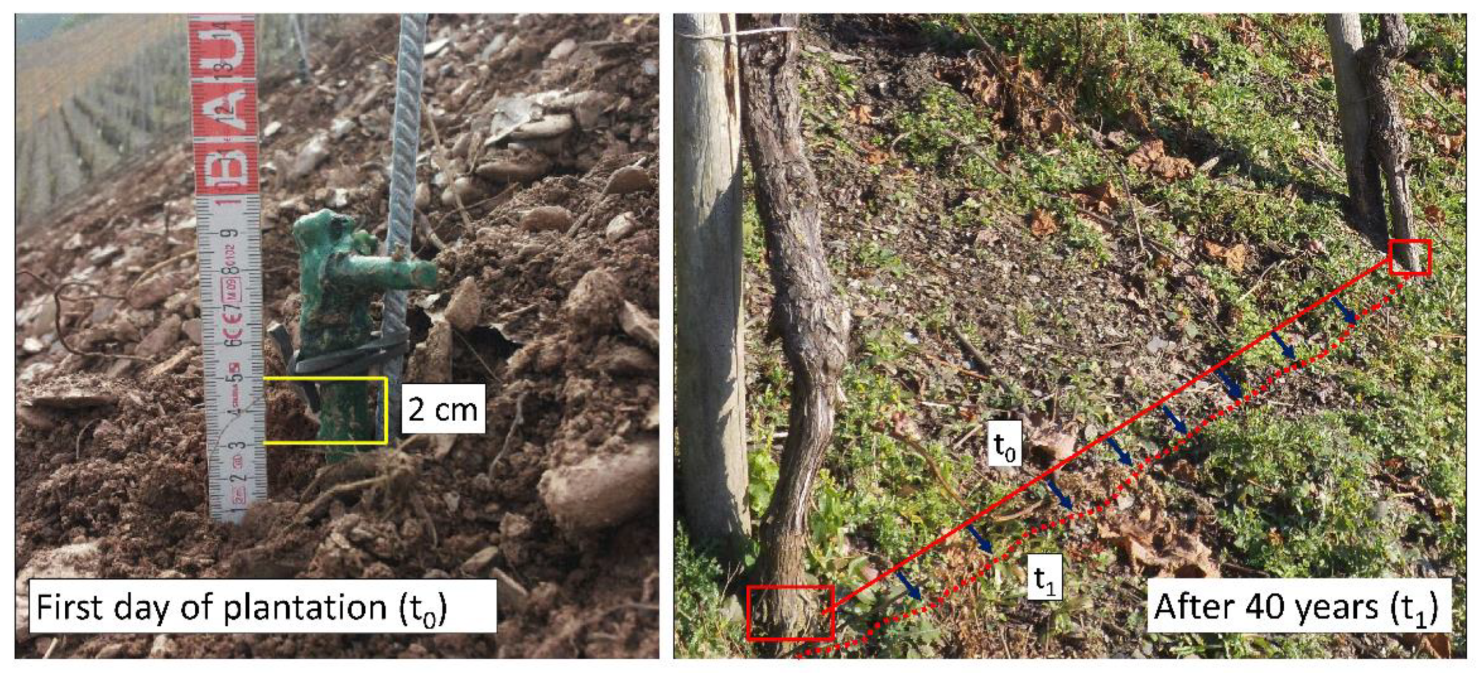
27]. For this study, the first step was to collect information about the plantation systems of our plot. The studied vineyard in Waldrach was manually planted and the graft unions were regularly situated 2 cm above the original soil surface level (
Figure 3). Prior to planting, the surface was mechanically flattened and the vine roots were then planted into the soil. This information was confirmed by the farmers in the field, the governmental advisory board DLR (Dienstleistungszentrum Ländlicher Raum) Mosel, and it was also observed in new plantations in the surroundings of the study area [
2]. Therefore, the possible changes from the theoretical initial soil surface conditions since the time of plantation commencement due to soil movements could be quantified. The separation between the graft union and the surface eliminates problems associated with high soil moisture, freezing, and fungi plagues, to the plants. In each paired-vine, the American graft unions were identified and a measuring tape was stretched horizontally between pair unions. The vertical distance between the horizontally stretched measuring tape and the current soil surface were measured with a meter stick. In cases where the graft union would have been buried, the measuring tape was situated at 30 cm above the graft union. This action was necessary to avoid difficulties in combining measurements between buried (positive values, an indication of accumulation) and unburied (negative values, an indication of depletion) grafts.
To eliminate systematic bias, it was important that the same person carried out all of the distance measurements. A total of 20 graft unions, 10 on each row of two opposite pair-vine rows 1.7 m apart with an inter-plant distance of 0.9 m, were selected for this experimental approach. The total plot area of 20 m2 (10 m long and 2 m wide) includes margins of 0.5 m at the ends and 0.15 m on the sides of the two-opposite paired-vine rows. The addition of the margins was to allow the assessment of the possible influence between vines, which is usually obviated by SUM and ISUM. If a grass cover made the visibility of the graft union impossible, it was carefully cut.
To compare the results obtained by the combination of SUM and SfM, ISUM method involving 19 (2 graft unions and 17 extra inter-row) measuring points per opposite pair graft union cross section was also used to generate the current soil surface map. The measured data were used to develop a soil surface level map using ArcMap 10.5 software (ESRI, USA), after creating a grid of 190 measuring points (“fishnet”). Different methods, such as cokriging, empirical Bayesian kriging, local polynomial interpolation and inverse distance weighting, were tested to identify the micro-topographical changes. Finally, the simple cokriging was selected because it showed the lowest root mean square error (RMSE) and the highest R2 coefficient.
2.3. Structure-from-Motion (SfM) Photogrammetry
SfM provides a perfect opportunity to survey any terrain of interest by taking a sufficient number of photos from specific positions [
28,
29], to develop a continuous point cloud. The point clouds of specific different sampling points in time, when the measurements were made, are subtracted in order to achieve a Digital Elevation Model (DEM) of the difference [
30]. In this paper, it is shown how to obtain a model of soil erosion by comparing the model of the actual soil surface with the hypothetical bulldozer-flattened surface derived from the SUM [
31].
While the SUM-derived ideal flat soil surface can be described easily, the actual surface with its micro-topographical surface irregularities has to be assessed with a sufficient resolution best achieved by means of an SfM. This sufficient overall resolution must be obtained according to the size of the targets. The lowest limit of resolution must, therefore, be closely connected to the range of the target´s sizes which is assumed to lie between soil aggregates to the little stones typical of vineyards on Mosel valley slates [
32]. This leads to dimensions from square millimetres to square centimetres, which indicate the maximum limit of the required potential resolution. In order to get a solid basis to start from, we called this premise “The best pictures, the best 3-D-model”. Corroborating with other researchers, the quality of the 3D-model strongly relies on the quality of the photoset [
33,
34]. To achieve this goal, we designed the TEPHOS (TErrestrial PHOtogrammetric Scanner).
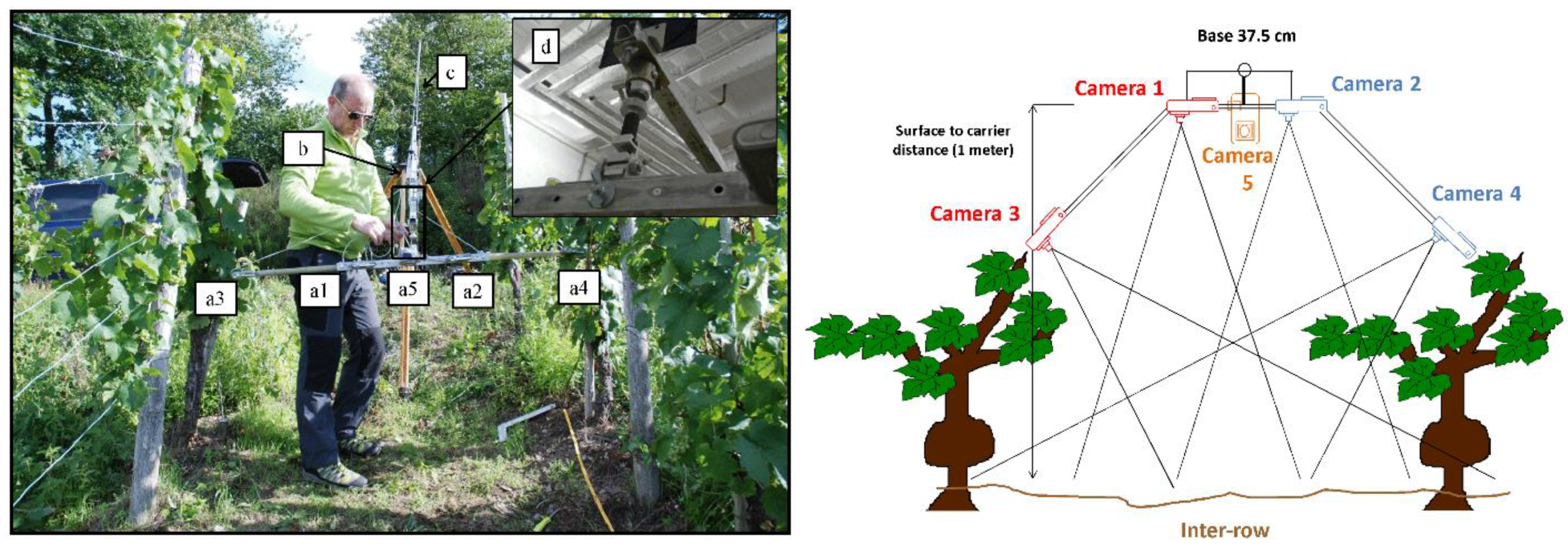
2.3.1. TEPHOS (TErrestrial PHOtogrammetric Scanner)
The TEPHOS can be defined as a static five camera array based on our design. In
Figure 4, it is shown the TEPHOS in action in the study area. In order to keep the device affordable, multiple Nikon L2 cameras (
Figure 4a1–a5) were used to get perpendicular and oblique views of the vine rows and inter-row areas. The cameras are characterised by (i) a 3× Zoom-Nikkor lens with 6.3–19.2 mm format equivalent to approximately 38–116 mm); (ii) an f-stop/3.2–5.3; (iii) lenses grouped into five elements and in five groups; (iv) 6.0 million effective pixels; (v) a sensor format of 1/2.5 inch and a sensor size of ~24.71 mm
2 (5.76 mm × 4.29 mm); and (vi) an approximate pixel pitch of 2.05 microns. All cameras were synchronised by a purpose-built tethered remote-control unit, which also serves as constant power supply and is fed by a 12 V/48 Ah car battery.
The cameras are placed on a horizontal aluminium rail that has several bores in symmetrical configuration to adapt the device to different photogrammetry-related requirements like overlap, depth of field, and others. The rail is mounted to a telescopic arm with a maximum range of approximately 3.5 m (labelled as b in
Figure 4) by a spherical joint to achieve a gimballed system (labelled as c and d in
Figure 4). The connection between the telescopic arm and the survey tripod is by clamping. The structural engineering calculation follows the example of a construction crane. Therefore, the heavy camera array on the long arm is compensated for by the weight of the relatively huge car battery. All parts of the TEPHOS were made of non-magnetic materials such as PE and aluminium in order to avoid a biasing effect on the electronics of the cameras. Other requirements on SfM serviceable photos had to be implemented as well. Ideal crop and suitable scale, which are questions of focal length, correct exposure, high contrast, sufficient sharpness, enclosing depth of field (all questions of shutter-speed and aperture), were ensured prior to taking photographs. In addition, minimum blur and hemispherical exposure positions were dealt with. All these demands were fulfilled by the mounted camera device. To improve the accuracy, a fixed array of five Nikon L2 cameras was used. The spatial interval of taking a series of synchronised photos in longitudinal direction downslope was defined as 10 cm. Herewith we acquired the lowest possible shutter speeds and, by means of systematisation, we reduced the post-processing time. The crisp sharp pictures and the sufficient overlap in both directions avoided data gaps.
In addition to the photo sets acquired with the TEPHOS, a Nikon D80 camera (with AF-S NIKKOR 18–70mm ED DX lens) was used to manually take photos from intricate parts where it was uncertain whether all the surface areas had been entirely recorded. The resolution of the Nikon D80s’ sensor is 3872 × 2592 (pixel size of 6.19 × 6.19 µm) with a focal length of 18 mm. In total, about 800 photos were taken in the field.
In order to get an appropriate DEM, a cloudy day was chosen to avoid casting shadows by direct sunlight, which could aggravate the processing of the photosets. Moreover, the grass cover between the vine stocks was removed by hand to get an undisturbed view of the soil surface.
2.3.2. Image Treatment Using AGISOFT Photoscan and CloudCompare
In order to compare the actual surface (t
1) to the initial one (t
0, representing the time of initial vine plantation), the photosets (t
1) had to be converted into a point cloud. To do this, we used a Lenovo Think Station S30 with double GPU Nvidia Quadro K4000 and 64MB Memory, and an SSD (Solid State Drive). The photosets were processed with AGISOFT Photoscan (AGISOFT, version 1.3.5., Russia) following similar procedures designed by [
35,
36], and CloudCompare (Telecom ParisTech, version 2.1., France). Another advantage is the processing system, especially, while handling big photo sets. For our studied vineyard survey of 10 m length, we had to process around 600 to 800 pictures, which took 3–4 days in total, a time that would have been lost, if the software did not process flawlessly.
First, AGISOFT Photoscan was used in order to compute the 3-D-models. This software is able to perform the photogrammetric processing of digital images and the generation of 3-D-spatial data and the calculation of the corresponding propagation of uncertainty. This procedure can be made performing the extraction and matching of key points, the orientation of the cameras, triangulation and creation of the point clouds. The adjustment of the controlling elements was always aimed to get the highest possible accuracy. This even meant that all six photo sets had to be copied onto the dedicated SSD for higher computing velocity (five photosets come from the TEPHOS‘s fixed array and one from the Nikon D80 DSLR). The procedures of the image treatment were as follows: (i) adjusting preference settings and loading photos from all six cameras; and (ii) aligning all photos, optimisation of camera alignment, and building a dense point cloud.
In order to make the point cloud measurable, we also circumferentially inserted 62 markers (meter tapes) and combined them with 34 scale bars into the soils between the vines. The whole problem area of calibration was handed over to the Photoscan adaptive camera model fitting function because any pre-calibration of our motorised zoom lens cameras would have only lasted until the first focusing. We used the function “placing markers” provided by AGISOFT with markers spread all around the plot. These signals were combined to scale bars. In addition to this, all the pictures from the five Nikon L2 cameras had been treated with the same calibration parameters by AGISOFT Photoscan because of the identical metadata concerning their camera type.
For measuring purposes, we imported the dense point cloud into CloudCompare. The next step was to horizontally align the cloud which enabled the colouring by height. The aligning job was initiated by fitting a plane to the point cloud. In the console window of CloudCompare, the position of the inserted plane (including translations and rotations) was displayed in the form of an editable transformation matrix. This matrix was used to transform the original point cloud to the horizontal plane. After visually checking, the exact adjustment of the inserted plane according to the positions of the graft unions in the point cloud was done. The final step, involving the colourising by height, was enabled by exporting the Z (vertical) coordinates into a scalar field.
2.3.3. Estimation of Volume of Soil Mobilisation and Soil Erosion Rate
To map the volume of the eroded material, we imported the aligned point cloud (*.ply): Polygon File Format or Stanford Triangle Format) into CloudCompare. Then, we inserted another plane which represented the initial surface levels at the date of initial vine planting and adjusted it according to the positions of the graft unions in the point cloud by editing the spatial properties of the plane. The next step, the colourising by height, was carried out by exporting each difference value to the new scalar field and then customising its colour ramp.
This scalar field of vertical coordinates is the basis for the final volume calculation by (i) fitting one plane, if possible, or (ii) fitting several plane segments which will better cover the successive lines of the graft unions. Following the stock unearthing method, we created a polygon crossing each paired-vine graft union. A total of four polygons were added covering the entire area with the help of the polyline function. The operator had to connect the side-lines of the segments to the graft unions. The polylines delineated the tetragons of the model in which a single volume calculation took place. After reckoning the individual volumes for every plane segment, they were summed up to work out the total volume. Finally, the total soil mobilisation of this transect could be estimated in Mg ha
−1 yr
−1 using the measurements from the volume difference between t
0 (polygons) and t
1 (soil surface map). The total soil mobilisation was calculated from the erosion-deposition (ER) equation proposed by [
26]:
where V (m
3) is the volume, S (ha) is the total surface for the considered field unit, A is the age of the vines (40 years-old) and BD is the soil bulk density (1.4 g cm
−3). The soil bulk density was obtained as the mean from 36 soil samples collected along the hillslope in different slope positions.
3. Results and Discussion
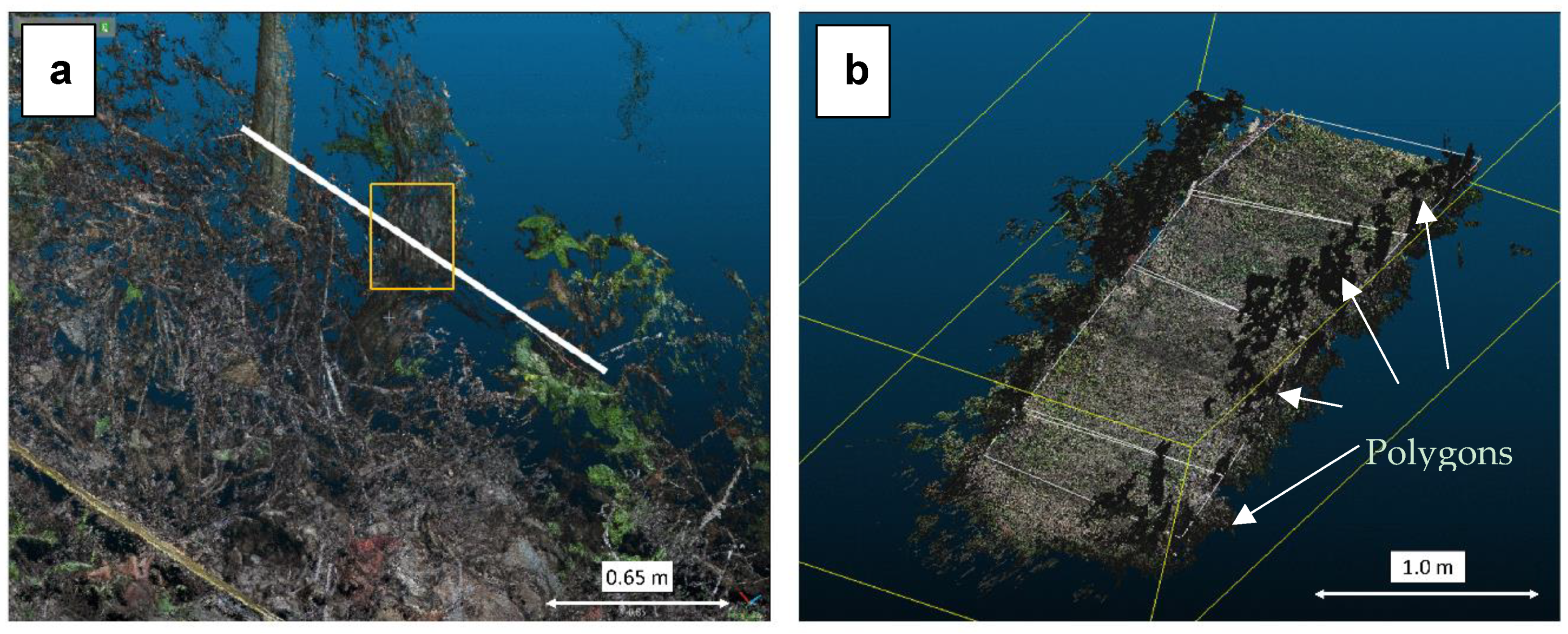
3.1. 3D Model Obtained from TEPHOS and Localisation of the Graft Union
The results of computing the actual soil surface illustrate a continuous DEM of the 10 m plot of a total area of 20 m². The initial visual inspection showed no extensive data gaps. A total of 638 out of 800 photos were processed by AGISOFT Photoscan to create 5,414,868 tie points. Altogether 12,871,537 projections with a reprojection error of 0.307 pixels were obtained (ground surface pixel area 0.625 mm × 0.625 mm). In the end, the dense point cloud consisted of 375,821,848 points. The final 3-D model is presented in
Figure 5. We have presented the 20 m
2 segment of the study plot and three screenshots of different slope positions. Moreover, three extra pictures with even higher zoom were added in order to demonstrate the accuracy of the obtained model, which can be emphasised by a mean point density of 18,791,092 points per m
2.
As other researchers have mentioned, there are a lot of obstacles in generating a model without gaps, including the shadows due to the vegetation cover, leaves and stones [
37]. In some transects close to the plants, this situation sometimes made it difficult to conduct the measurements. However, the combination of the TEPHOS (5 cameras) with the hand-held Nikon DSLR (1 camera) enabled us to manage these problems. We believe, that the systemised usage of the fixed array cameras prevented us from taking either too many or too few photos. Too many pictures would mean extended computation time, whereas too few pictures would result in data gaps.
One disadvantage was observed during the fieldwork, this being the demand for storage and transport space for the TEPHOS, especially if all the equipment had to be carried by the operator in such a difficult terrain. Also, we noted that managing the more than 300-million-points point cloud was another issue that should be looked into in the future. For example, we could take less but more demand-oriented pictures and use a more powerful computer. We recommend the number of points in the point cloud be decreased in order to speed processing time. Thus, a systematic test should be done to assess how many photographs/points are needed to maintain the required accuracy of the soil erosion estimate. This would speed up the next investigation and data processing and would be of interest to those of the SfM community who decide to work with this combined method.
After that, following the indications of the authors that worked on the stock unearthing method, we created a polygon crossing each paired-vine graft union. A total of four polygons were added covering the entire area (
Figure 6).
3.2. Soil Surface Level Assessment and Soil Mobilisation Rates
The computation of the relative height map was done in order to calculate the total volume of mobilised soil in the study area during the 40 years using SfM and SUM. This map also shows key information related to the connectivity processes, which allow us to assess flow paths, accumulation points or pools [
38,
39].
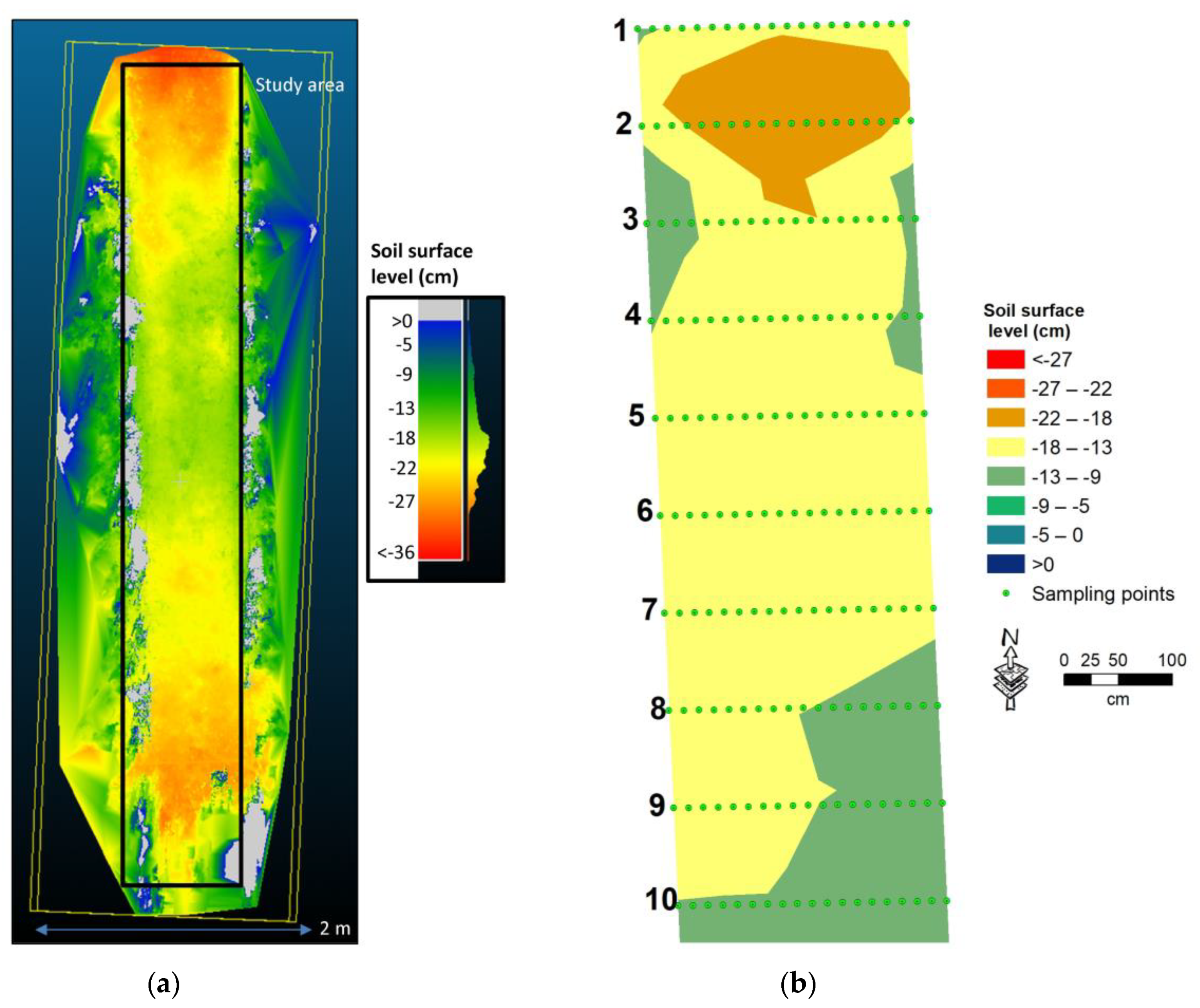
Figure 7a shows the final map of the relative height used to assess the micro-topographical changes, which is more accurate than the map created by ISUM (
Figure 7b). Grey colours in
Figure 7a represent areas with a relative height of zero or higher. Note that with ISUM, the graft union locations and the inter-row measuring points appearing as green dots were used and interpolated over the entire plot in
Figure 7b.
In both maps, we detected that the highest depleted areas are located in the upper part of the transect (orange-red colours) reaching values higher than 20 cm, and in the areas close to the vine rows (orange-yellow colours). Our results corroborate with other researchers who found these parts to be the most eroded areas due to wheel or chain traffic effects [
40,
41] as a result of gravitational processes [
42]. Conversely, the areas with the lowest soil depletion are situated in the middle part of the plot, unaffected by the tractor impacts and also non-compacted [
43].
Using the photogrammetric technique, the total soil volume mobilised from the study area was 0.52 m3, and, using the bulk density value of 1.4 g cm−3 we obtained a soil depletion rate of 9.14 Mg ha yr−1. In contrast, the ISUM method gave a total depletion volume of 1.86 m3 leading to an unreasonable depletion rate of 40 Mg ha yr−1.
It is important to remark that the bulk density estimate is for a specific sampling time and the number of sampling points will determine the representativeness of the actual rates. Regardless, the bulk density values were used only to obtain a comparable result in one of the most common units (Mg ha yr
−1). As is well-known, the bulk density is a soil property that can vary after rainfall events, tillage practices or changes in organic carbon contents among others, although the variation may not be extreme [
44,
45]. However, in order to avoid any over-or under-estimation, the use of volume can also be an acceptable unit as used in other studies [
14,
31].
Considering that our results correspond to a small plot using a photogrammetric technique, the registered soil erosion rates are not significantly different from those reported in other studies in Germany. Using empirical methods such as RUSLE (Revised Universal Soil Loss Equation), References [
46,
47] estimated within the same viticultural region (Ruwer-Mosel Valley) values of 6.47 and 11.28 Mg ha yr
−1 over some years. Also, for several German vineyards, Reference [
48] calculated an average value of 5.2 Mg ha yr
−1.
3.3. Challenges and Future Lines
Combining SfM and SUM for the estimation of long-term erosion rates is the most important achievement of this investigation. In this paper, the combined methodological approach is a proof of concept as it was applied to a small plot. The intention is to apply the method on a much larger scale at a later date to inspire others for uptake in vineyards.
Table 1 compares the main advantages and disadvantages of SUM and ISUM and highlights issues that have been improved or even solved by the combination of SUM and SfM. This paper focused more on SfM, considering that the graft union can be easily identified in the same data with high accuracy because they are visible in images, which may not be easily identified in LiDAR point clouds, as shown by Reference [
38] for example at the larger scales. We consider the easy identification of the graft unions is a major advantage for SfM over the use of LiDAR in vineyards, especially considering the lower prices (drones vs camera-array), higher accuracy (e.g., RIEGL VZ-400i: accuracy of 5 mm) and time required in the field.
The main issue solved was the detection of the soil surface components such as stones, and remains of leaves and grasses. On the whole, we consider our results as very positive and accurate, making the detection of previous micro-topographical changes very easy.
Our novel approach to detect the micro-topographical changes uninterruptedly with the consequence of a huge number of points (more than 375 million) and software limitations may make it difficult to statistically assess the values obtained. For example, calculation of the mean, maximum or minimum values as other authors have done [
47,
49]. Therefore, further research must be done in order to implement these kinds of calculations to make our results directly comparable to those in the literature. Data analysis should be implemented to improve the use of both methods.
4. Conclusions
By using the combination of SUM and SfM, we found that a total of 0.5 m3 of soil was mobilised on a 20 m2 plot over a period of 40 years. For this small transect, ISUM overestimated the total volume of mobilised soil (1.86 m3). With the combined method, we could monitor the soil surface differences in the upper part of the study area from the initial level to the current one in excess of 30 cm.
The combination of stock unearthing method (SUM) with the Structure-from-Motion Photogrammetry (SfM) has been verified as a very efficient non-invasive method for monitoring long-term soil erosion in vineyards. The main shortcoming of ISUM, namely not being able to scan all areas between opposite pair vines, is overcome by the TEPHOS, an SfM method. TEPHOS (TErrestrial PHOtogrammetric Scanner) allowed us for the first time to scan an entire 20 m2 plot located within a steep sloping vineyard of the Ruwer Valley, Trier (Germany). An easy and low-cost method to estimate soil erosion in vineyards with very high spatial resolution has been presented. With this method, we can demonstrate the importance of soil erosion as a severe environmental concern for farmers in a convincing manner. This argumentation aid may hopefully help us to persuade the owners of particularly steep sloping vineyards to undertake erosion control measures.


 ,
, 


