Optimising Citizen-Driven Air Quality Monitoring Networks for Cities


1
Westfälische Wilhelms-Universität, 48149 Münster, Germany
2
NOVA Information Management School (NOVA IMS), Universidade Nova de Lisboa, 1099-085 Lisbon, Portugal
*
Author to whom correspondence should be addressed.
ISPRS Int. J. Geo-Inf. 2018, 7(12), 468; https://0-doi-org.brum.beds.ac.uk/10.3390/ijgi7120468
Submission received: 31 August 2018
/
Revised: 23 November 2018
/
Accepted: 27 November 2018
/
Published: 30 November 2018
(This article belongs to the Special Issue Volunteered Geographic Information: Analysis, Integration, Vision, Engagement (VGI-ALIVE))
Abstract
:Air quality has had a significant impact on public health, the environment and eventually on the economy of countries for decades. Effectively mitigating air pollution in urban areas necessitates accurate air quality exposure information. Recent advancements in sensor technology and the increasing popularity of volunteered geographic information (VGI) open up new possibilities for air quality exposure assessment in cities. However, citizens and their sensors are put in areas deemed to be subjectively of interest (e.g., where citizens live, school of their kids or working spaces), and this leads to missed opportunities when it comes to optimal air quality exposure assessment. In addition, while the current literature on VGI has extensively discussed data quality and citizen engagement issues, few works, if any, offer techniques to fine-tune VGI contributions for an optimal air quality exposure assessment. This article presents and tests an approach to minimise land use regression prediction errors on citizen-contributed data. The approach was evaluated using a dataset (N = 116 sensors) from the city of Stuttgart, Germany. The comparison between the existing network design and the combination of locations selected by the optimisation method has shown a drop in spatial mean prediction error by 52%. The ideas presented in this article are useful for the systematic deployment of VGI air quality sensors, and can aid in the creation of higher resolution, more realistic maps for air quality monitoring in cities.
1. Introduction
Air pollution is currently a global fret, which can be linked to the extensive population growth and urbanisation, together with their aftereffect in traffic, industrialisation and energy consumption [1]. Human health is closely linked to the air we breathe [2], as evidence from recent studies for the adverse health effects has shown [3,4]. A recent report of the World Health Organization (WHO) suggests that 92% of the world’s population lives in places that exceed the recommended annual mean concentrations of Particulate Matter () [5]. Because of the growing health effects of chronic exposure to ambient air pollution, policy makers and scientists are showing an increased interest in monitoring air pollution at a higher spatial resolution. Various recent studies from spatial epidemiology and public health have set out a specific interest in traffic based pollution [6,7,8], particularly in Stuttgart, Germany [9]. Generally, air pollution monitoring is done by environmental or governmental organisations using a network of fixed monitoring stations. Typical regulatory decisions are taken based on long duration temporal trends and statistics [10], considering conditions related to hotspots estimated based on real-time data, if available. Interpreting the pathways from the generation of emission, dispersion and chemical transformation of pollutants in ambient air pollution concentrations is very challenging due to its high spatiotemporal variability [11]. In the recent years, land use regression (LUR) has been widely used in various health and epidemiological studies to estimate air pollution at a finer spatial scale in the urban areas [12,13,14]. However, due to economic reasons, the number of air quality monitoring stations in cities is usually sparse and limited, and this considerably limits an accurate assessment of the intraurban variability of air pollution.
Citizens and environmental agencies are exploring the potential of small, low-cost air quality monitoring sensors to enable detailed real-time information on air quality in the city [15,16,17]. Several low-cost sensor deployments have been conducted in recent years extending from citizens investigating air quality in the houses and surrounding areas, to networks of sensors to measure community-level air quality, to a vast network of sensors covering the cities [15,18]. However, the datasets provided by low-cost sensor networks are arguably of less accurate [19,20,21]. Despite such a limitation, the demand for sensor technology is high, driven by widespread concerns about the air pollution as well as an interest in reducing the personal exposure [22]. While crowdsourcing approaches for air quality data gathering and related technologies are escalating, research to inform the translation of low-cost air quality sensor data into real applications remains limited. The term “low-cost” might be interpreted differently depending on the end users and the specific purpose of the study. For instance, U.S EPA Tier 3 instruments can be low cost (2000–3000 USD) for regulatory authorities but not for general citizens who are willing to participate in the data collection process [23]. Therefore, in our study, we refer to low-cost sensors as devices which cost less than 200 Euros (and can thus be used by individuals or communities for air quality monitoring).
To capture the spatial variability in detail, accuracy of data will profoundly be relating to “where” the data are collected. To better understand exposure in microenvironments, it is crucial to take into account the spatial coverage of air pollution monitoring networks. Inappropriate location selection may lead to over- or underestimation of pollution originated from various emission sources in the city. When considering low-cost sensors to gather air quality data, previous studies suggest that, generally, the datasets generated with the help of citizen or community participation approaches inherit serious data gaps and the measurements collected are from irregularly spread sensors [21]. Since the process of air pollution monitoring to capture spatial variability involves specific cost and time [24], it is desirable to optimise the monitoring locations. Hence, to overcome the data gaps and irregular spatial spread of sensors to make data collection more efficient, there is a need for methods that can help in extending wide-spread and optimal location identification.
Participatory data approaches can be helpful to enable detailed air quality data collection, but exploiting the datasets generated from these low-cost devices requires tools and techniques for data cleaning and processing. The vast amount of dynamic, varied, detailed, and interrelated datasets from citizen participatory approaches could be enhanced by preparing the protocols and infrastructure that enables scientifically sound data collection [25]. The systematic deployment of low-cost sensors for urban air quality monitoring can be useful for air quality data collection. With the potential of low-cost air quality monitoring sensors to increase the spatial coverage [26], along with its application to foster participation [22], it is desirable to systematically identify the optimal placement of monitoring stations to make the best use of advanced sensor technology and citizen engagement efforts.
The present study aimed to develop a method which can help in systematically identifying the optimal locations of citizen sensors for air pollution monitoring. The method was tested using citizen-contributed data from the city of Stuttgart, Germany as a scenario. The primary objective of the optimisation method included the identification of the most advantageous spread and optimal monitoring site locations that minimise mean prediction error for land use regression (LUR) estimations of air quality parameters for the study area. LUR is a method for spatial exposure assessment. It helps to model pollutant concentrations (e.g., particulate matter and nitrogen dioxide) at any location using various environmental characteristics of the surrounding area (e.g., traffic intensity, elevation, and land use type). The spatial simulated annealing (SSA) algorithm was used to run the objective function for finding the optimal monitoring network design.
The main contributions of this study can be summarised as follows:
- We extended the optimisation method proposed by Gupta et al. [27] by incorporating wide-spread distribution aspects (in addition to LUR’s predictor error aspects) into the placement of low-cost citizen sensors for air quality monitoring.
- We demonstrated the applicability of the proposed optimisation method in two practical scenarios: starting a new volunteered geographic information (VGI)-based air quality monitoring campaign; and finding out where to place new sensors to extend the existing VGI-based air quality monitoring network from the city of Stuttgart, Germany.
While existing works on analysing the quality of VGI mostly aim at examining the degree to which a fact contributed by a volunteer is likely to be true (see, e.g., Goodchild and Li [28]), this work approached the question of quality of VGI from a slightly different angle. By trying to find the spatial distribution of volunteers which can minimise the global prediction error of the air pollution monitoring network, this work intended to inform the coordination of VGI efforts for air pollution monitoring at the city level. As such, the method proposed can be classified as belonging to the fourth type of VGI validation process identified in [29], namely “measure of fitness by way of completeness” (not the amount of points, but the promise of detail or spatial extent). There are a couple of methods in the literature to tackle the VGI quality aspects of positional accuracy, thematic accuracy, and topological consistency, but a general lack of methods addressing other aspects such completeness, temporal accuracy, or vagueness, as a recent review by Senaratne et al. [30] reminded. Criteria such as road density or errors of omission/commission are used as surrogates for completeness in some studies [31,32], but completeness in this study was approximated using the combination of two criteria: spatial spread and minimal prediction error of the air pollution monitoring network.
The rest of the paper is organised as follows. In Section 2, we present a brief overview of the previously done work on the topic. Section 3 describes the study area and the data used in the study. A new methodology for optimisation is described in Section 4. In Section 5, we present the results and discuss the objective function used in the proposed optimisation method. Section 6 presents the discussion regarding the developed optimisation method. We draw the conclusion in Section 7.
2. Related Work
The deployment of the network of air quality monitoring stations is of vital importance for various air quality monitoring methods. Various air quality methods and their regulation exist in the literature, and the adoption of crowdsourced air quality data for filling data gaps has also been a topic of discussion in recent years (see, e.g., [33]), especially for the vision of the smart city and citizen engagement. This section briefly discusses previous related work on the topics of crowdsourced data integration approaches and air pollution monitoring.
2.1. Citizen Participation/VGI
The effect of pollution on city residents requires a monitoring network that can provide a representative view of the experiences across the population while considering the wide distributions of pollution levels and local socioeconomic conditions across the monitoring sites. Low-cost sensors can be helpful in advancing air pollution monitoring by gathering a massive amount of spatiotemporal air quality data. Various low-cost air pollution sensors have already been successfully integrated into long-term deployments to access fine-grained air pollution information [17]. In practice, these data sources can help in facilitating ongoing indications of changes in air quality, rather than absolute measurements [34]. The applicability of low-cost sensors for future air pollution monitoring is well recognised in the literature [16,20,22]. Extending the application of these sensors by involving citizens or communities for environmental data collection has increased in the recent past [22,35]. Through volunteered geographic information (VGI) or crowdsourcing data methods, a large number of individuals may be engaged to collect data about phenomena impacting the city life. In general (and as indicated by Lisjak et al. [36]), the involvement of citizens not only provides an opportunity to close data gaps but also brings the policy-making process closer to people. Citizens are willing to get involved in air pollution monitoring studies and get aware of the ambient environment [22,37]. With the help of citizen participation, hundreds of low-cost sensors can be dispersed in an urban environment that can facilitate data collection simultaneously. These gathered data can promote the development of improved models that can explain the pollutant variability within the urban environment.
Education and involvement of communities for air quality monitoring is not only crucial for improving public health but also for building awareness about the sources of air pollution, exposure causes and impact of other pollutants on health. Engaging citizens may also support in deploying the network of low-cost air quality monitoring sensors that can be of significant potential for improving the spatial coverage of pollutant’s variability in urban space and can foster citizen participation [22]. Despite these advantages, while utilising these alternative data sources, attention is needed to undertake valid capturing and representation of the data. The design of the air quality monitoring network is of vital importance for extracting precise and detailed spatial variability information of air pollution in the city. Most of the datasets generated with the help of citizen or community participation approaches suffer from serious data related gaps and the measurements collected are usually from irregularly spread sensors, which may represent the air quality for only a small number of areas [21]. The irregular distribution of air quality data acts as a barrier in utilising such observations for air quality mapping applications for the cities. Another important consideration while monitoring detailed air quality in the city involves the selection of monitoring sites and the number of sensors involved in an air quality monitoring network. The number of sensors involved and their locations can affect the expected outcome of the air quality modelling approaches that utilise the data specific modelling approaches [24,38,39,40].
The selection of monitoring site is challenging because of various parameters such as local land use type, emission source, electricity connections, installation requirements of the equipment and aim of the study. Increasing the number of sensors in the monitoring network also increases the costs and efforts for data process and information generation. Systematic location and size selection for sensor network deployment can be a useful consideration to gather the optimal volume of data with the proper spread as per the fitness of purpose. It is neither practically possible to gather air quality measurements at all locations in a city nor is it required. Few carefully chosen locations that can fit the purpose of the study with the specified number of sensors in the network can be helpful in representing the air quality for the city in detail. The necessity of formulating the requirements for low-cost sensor network deployment for the specific purpose and at a specific location is essential. Clements et al. [22] recommended the identification of the research question as one of the key consideration for planning the deployment of the citizen participation based air quality sensor networks. Their discussion suggests that the research question and pollutant(s) of interest should govern the size and locations of the air quality sensor network. For instance, if the aim of the study were to reliability measure air quality in a city over a large area (which is the primary focus of our study), sensor locations are important, but so are the data redundancy aspect, pollutant variation and sensor density within the network [22]. For the systematic deployment of the low-cost air pollution monitoring sensor network, we could combine the crowdsourced data location selection with scientific models and their variables, to achieve better spatial coverage.
2.2. Air Quality Monitoring Methods
Geospatial tools have become useful for modelling air pollution in recent years. To represent the intraurban variability of pollutants, various exposure assessment methods are proposed [8,10]. Approaches include interpolation of fixed-site monitoring stations, dispersion modelling, remote sensing, land use regression (LUR), proximity and various other deterministic methods [41]. Each method has their inherent limitations that may restrict their application for developing detailed air pollution maps for the cities. For instance, the dispersion models that simulate pollutants dispersion and reaction in the atmosphere are often infeasible at higher spatial resolution for larger areas [42]. The interpolation of pollution data collected by regulatory air quality monitoring stations can help in regional patterns identification, but the networks are very sparsely arranged to collect informed data, hence limiting their application for detailed air pollution modelling [38]. Over the years, LUR modelling has demonstrated better or equivalent performance to other geostatistical and dispersion methods and is therefore being considered for application in various epidemiological exposure studies [38]. However, the scarcity of sensor data may impact the outcome of LUR models. To address the sparsity and scarcity challenges, robust and compact systems that can be wide-spread are desired to capture the spatiotemporal variations of air pollutants [43].
Usually, the measurement of air pollution in urban space is possible with the help of a network of air quality monitoring sites. In practice, EU states are required to comply with the directive, framework and legal requirement for assessment and management of ambient air quality as described in the Air Quality Directive 2008/50/EC [44]. The methods for monitoring air quality currently involve the use of fixed monitoring station networks in the European cities. Monitoring of air pollutants is primarily performed using analytical instrumentation, such as optical and chemical analysers. However, installation of single monitoring stations will neither help effectively in monitoring air pollution [45] nor will the placement of monitoring stations ad-hoc or in few centrally located areas be adequate to infer the pollutants’ detailed spatial variability in a city [46]. The air quality maps observed presently are very scarce as the analysers used in the observation network are complicated, bulky and expensive, together with a significant amount of resources required to maintain and calibrate them [47]. These constraints lead to the low number of air quality monitoring stations that are generally not adequate to capture the small-scale spatial variability of air pollutants in the urban environment. As said previously, recent advancements related to sensor technologies have resulted in relatively low-cost and small devices for measuring air quality [48,49]. The emergence of low-cost devices is also recognised by policymakers and recommended to be embodied in the air quality directives [23,50]. Current air pollution monitoring networks can benefit from the use (and efficient spatial distribution) of these low-cost sensing devices in the context of volunteered geographic information.
Overall, crowdsourced data/VGI has a significant potential to improve current air pollution monitoring networks, notably through the provision of new data points to expand their spatial coverage. The spatial arrangement of sensors usually influence how well the spatial distribution of air pollutants and their impact can be captured [39]. Although various approaches have been proposed to identify the optimal locations for air pollution monitoring sensor placement [51], few studies focus on general location selection aspect for deployment of low-cost sensors [52,53]. To our knowledge, no previous studies have considered the application of an optimisation method to enable systematic location selection for robust LUR estimations during the crowdsourcing of air pollution data for cities.
3. Material
3.1. Study Area
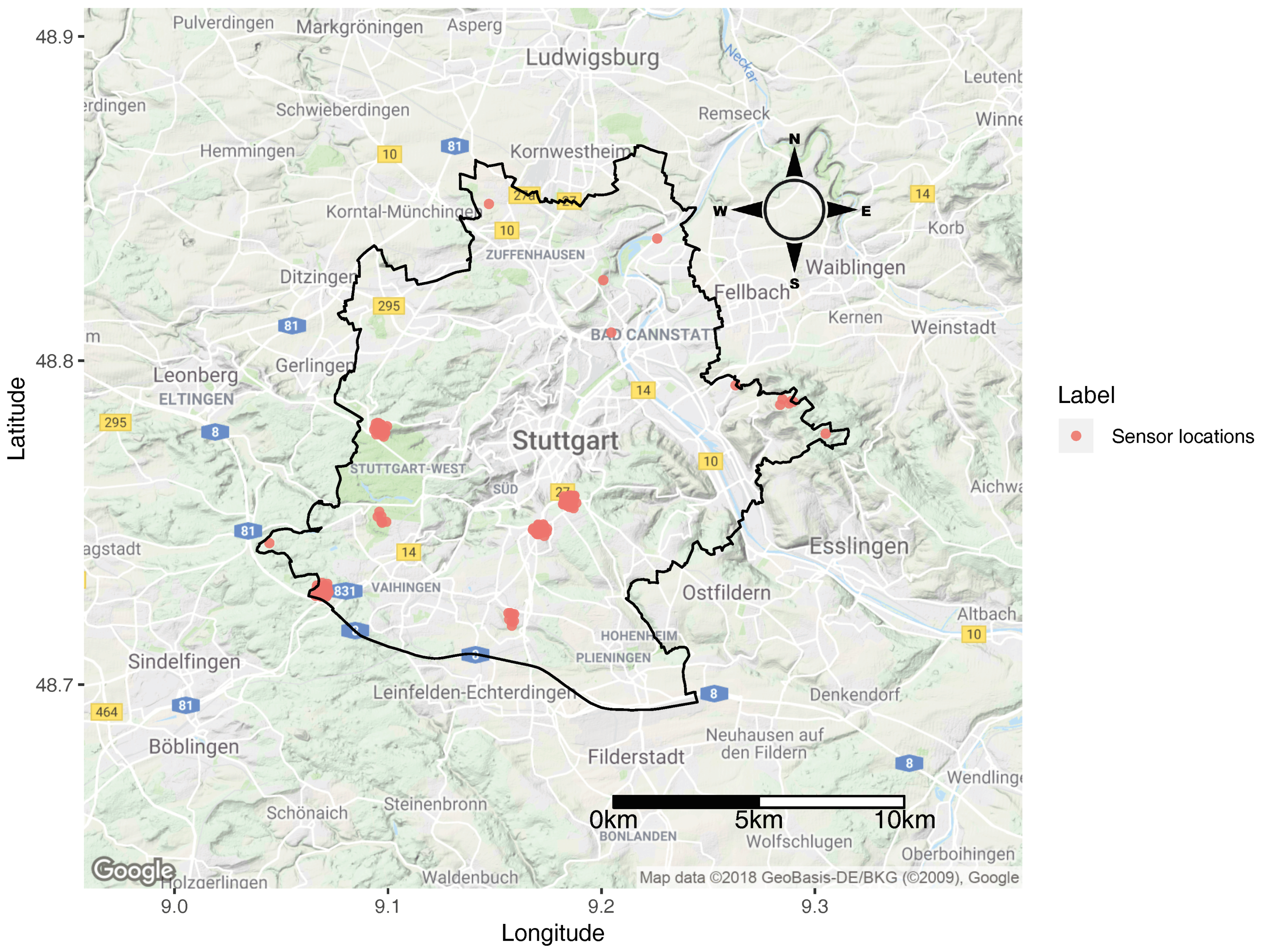
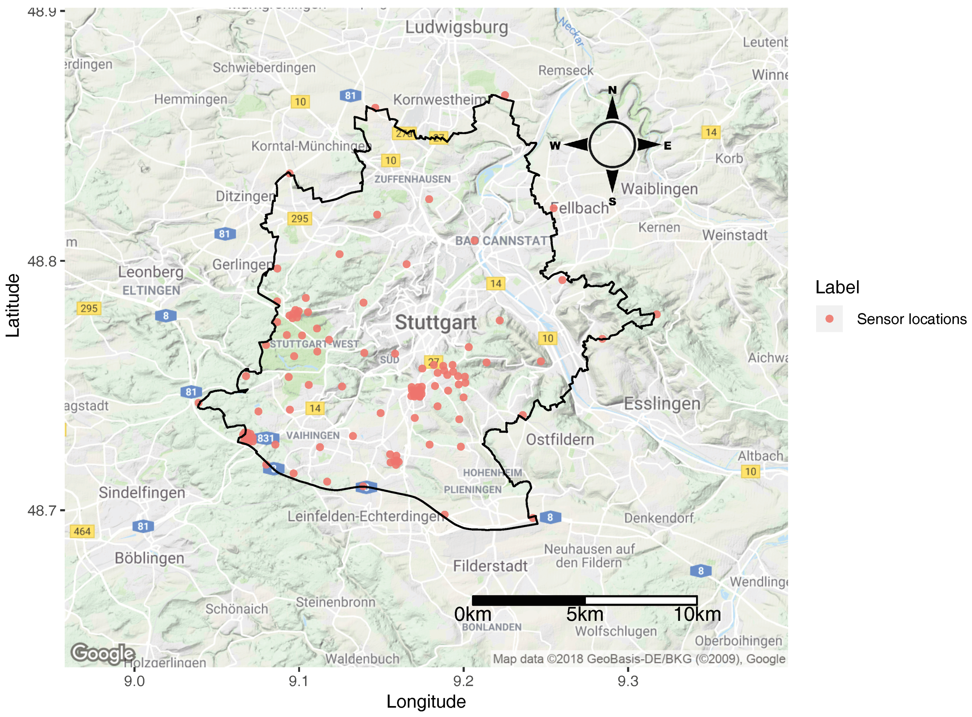
The proposed method was applied for the city of Stuttgart (48.7758° N, 9.1829° E) situated in the the state of Baden-Württemberg, Germany. The city of Stuttgart is also the capital of Baden-Württemberg state (population: 11 million; size: 36,000 square kilometers) and the Administrative Region of Stuttgart (population: 4 million; size: 11,000 km2). It is located at the centre of the very densely populated southwestern Stuttgart Region (population: 2.7 million; size: 3700 km2), close to both the Black Forest and the Swabian Jura. It covers an area of 207.35 km2 and lies in a bowl-shaped valley about 270 m above the sea level on the back of the Neckar River. The city centre is situated in a lush valley, ringed with vineyards and forests, and the river and has a population of 628,032 (as of 31 December 2016) [54]. Air pollution is a severe concern in the city due to its topographic conditions and industrialisation. Few German newspapers also call the city of Stuttgart “the German capital of air pollution” [55]. In 2016, the city authorities issued an alert, the first-ever warning in Germany concerning air pollution [56]. Currently, city environmental protection authorities are utilising four monitoring stations to gather data about air quality in the city [57]. Measurements from three out of four stations are available as open data. Figure 1 shows the locations of stations whose data are openly available on Umwelt Bundesamt portal [58]. Figure 2 presents the study area with the crowdsourcing sensor network.
3.2. Data
The sources of data that are used for this study can be divided into two categories, as detailed in the following section.
3.2.1. Citizen-Generated Air Pollution Data
Four official monitoring stations alone would not be enough to fully assess the amplitude of the air pollution issue in Stuttgart, as well as the effectiveness of measures taken to mitigate it. Fortunately, the city of Stuttgart has a dense network of citizen-driven low-cost air pollution monitoring sensors developed by OK labs [59]. Ground measurements of and from low-cost sensors are available as open data for various locations [60]. Initially, the data of 594 (the dataset does not allow for statements on the actual number of VGI contributors) sensors were downloaded for the first week of 2018 (1–7 January 2018). Further data cleaning for removing sensors with no values in the specified period and the pollutant of interest led to a final total of 116 monitoring sensors, which were used in this study. The measurements are collected using SDS011 sensors, with the measurement unit of μg/m3 [61].
3.2.2. Land Use Regression (LUR) Variables Open Data
A LUR model needs several geographical predictors variables (e.g., land use type, road count, distance to roads, traffic, and terrain variables for specific buffers around the monitoring stations) as input. In the modelling process, the air pollutant measurements were considered as the dependent variable, and geographical predictor variables were considered as the independent variable to establish a regression model that can help in estimating the air pollution at unmeasured locations. A linear regression model has an equation of the form:
where
- y is an n × 1 vector with air pollution observations at low-cost sensor locations for any particular instance (where, in our case, weekly mean concentration was used);
- X is an n × k matrix with observations of k independent variables for the n sensor locations;
- is a k × 1 vector with unknown parameters; and
- is an n × 1 vector of residuals, assumed to be distributed independently and identically.
The values about the predictor variables were extracted from the open data available on the Internet. The buildings and road datasets were downloaded from Open Street Maps (OSM) and Geofabrik services [62,63]; population data were downloaded using European Data Portal [64]; altitude data were downloaded from Bundesamt für Kartographie und Geodäsie open data portal [65]; and the land use data were downloaded from CORINE Land Cover (CLC) [66].
4. Method
As mentioned in Section 1, the present study sought to develop an optimisation method that can take into account fitness-of-purpose as objective for VGI data collection. As Clements et al. [22] suggested, the identification of the research question before planning the deployment of the VGI based air quality sensor network can help in useful data collection. The optimisation method presented below takes the question “what are the set of locations in the city where measurements are required for estimating air pollution with minimal LUR prediction error?” as the research question. It used Spatial Simulated Annealing (SSA) to run the objective function.
SSA is a random search algorithm that explicit deals with spatial vicinity. It is the spatial version of the probabilistic techniques simulated annealing, which was developed by van Groenigen [67] for spatial soil sampling design optimisation. The SSA technique mimics the cooling of metal phenomenon to reach global optima, i.e., simulated annealing. In the starting phase of the annealing process, the locations for sensors can change greatly, with low probability even at not so optimal locations. As the process cools down with time, changes in locations become smaller, and acceptance of worse designs of monitoring network becomes less likely. During the optimisation process, the algorithm takes several hundred or thousands of iterations to identify the optimal configurations. The SSA algorithm is widely used in sampling design for mapping [67,68]. The SSA algorithm requires an objective function, whose output value acts as “energy” in the optimisation process. The optimal design identification is made based on the set of the location which represents the minimal energy of all iterations in SSA. Hence, the objective functions should be formalised as a single objective optimisation function, pointing at discrete-valued variables which calculate the energy value.
4.1. Optimisation Objective Function
The optimisation was performed based on some rules and objectives that are used as a function. The optimisation objective function is usually composed of one or many constraints, which were calculated using the explanatory variables of a given LUR model in our case. The objective function was implemented using SSA, where it estimated the objective function value (also called the energy of annealing) to identify the set of locations which fulfil the given optimisation objectives. The objective function used in our study considered two aspects:
- prediction error; and
- widespread distribution aspect.
4.1.1. Prediction Error Aspect
The first aspect of the objective function was adopted from the previous work done by Gupta et al. [27] to identify the set of locations for crowdsourcing sensors which collectively can help in modelling concentration with the less spatial mean of prediction error for the study area. The prediction error is the measure of the accuracy of the model to predict the value of the variable of interest by using various independent variables. The prediction error aspect of the objective function considered the covariates of the selected LUR model that can help in estimating the concentration in the study area. The evaluation of the prediction error was done considering the matrix approach for the least squares estimate of linear regression:
where and represent the predicted and measured value of the dependent variable; , …, represents the vector of the set of predictor variables values at the prediction site; represents the transpose vector; and X and are the matrix and transpose matrix of the predictor variables for the randomly selected monitoring site.
is the residual variance of the regression, which is constant [69] and independent of sampling locations. Hence, it can be left out of the objective function. The average predicted error of the LUR model is thus proportional to:
and that is what we use as objective function.
For a two-dimensional study area A (represented by the number of its grid cells), the prediction error aspect is computed using n observation sites for a network design D. D is the design of the set of monitoring locations identified at each iteration of the optimisation process. The optimisation process starts using a network configuration fed in as input or by randomly selecting monitoring design , consisting of observation points with corresponding predictor variable vectors , …, . During the optimisation process, the monitoring sites are transformed into a random vector with only one element different from the initial one, yielding a new monitoring design . The optimisation process computes the prediction error for each (x ∈ [0, …, n]) utilising each node of the rasterised study area A, until the minimum value is achieved using , …, , which represents the set of predictor variables values at prediction location in A, with X and being the matrix and transpose matrix of the predictor variables for the randomly selected monitoring network design (x ∈ [0, …, n]) in the optimisation process. For the objective function, the manipulation of the set of locations leads to the modification of X matrix values. For further details about the above-mentioned objective function, we suggest referring to the work done by Gupta et al. [27].
4.1.2. Widespread Distribution Aspect
Along with the requirement of the objective function to decrease the mean prediction error for the study area, the second aspect in the objective function focuses on enforcing the wide-spread distribution of sensor network in the study area. A wide-spread deployment is necessary because it can help in providing higher spatial resolution to air pollution data, which in turn better informs the identification of pollution sources and supports more conclusive studies on the effect of air pollution on the quality of life in cities [70,71]. A widespread deployment also helps in reducing the uncertainties associated with the modelled forecasting results.
Many low-cost sensors involved in the optimisation process along with uncertainties that can be caused by the spatial autocorrelation of the predictor variables used for optimisation may lead to clustered results. Furthermore, the selection of locations with extreme values of predictors in the optimisation process, while only considering the prediction error aspect, can also lead to clustered results. It is essential to have a constraint which can limit the clustering and enforce the selection of disparate locations. Hence, we extended the objective function developed by Gupta et al. [27] to take into account the wide-spread distribution aspects of sensors in VGI-based monitoring network design.
To integrate the wide-spread aspect in the optimisation objective function, we calculated the inverse mean shortest distance (IMSD) for the set of locations selected in each iteration of annealing after calculating the mean prediction error value considering Equation (3) in the optimisation process. The spread aspect of the objective function can be written as:
where N is the number of points in the configuration considered for optimisation and is second minimum distance between the ith point and other points of configuration (as the minimum value will be 0 for each point distance to itself).
The algorithm for computing the IMSD (Equation (4)) to enforce wide-spread distribution of sensor locations (as points) can be summarised as:
- Input of a number of points (N) with a different spatial configuration as selected in each iteration of SSA.
- Compute the distance matrix for all points.
- Identify the second minimum value in each row of the matrix, as the distance matrix will contain the first minimum value as 0.
- Compute the mean of the minimum values from each row and column of the distance matrix.
- Compute the inverse of the mean value.
After the computation both aspect values using Equations (3) and (4), the values are then added to get a single objective function value which is further characterised as energy state in the SSA optimisation process. Furthermore, the optimisation function was made flexible to consider the weight function to prioritise one of the two aspects (prediction error or spread function) when identifying optimal locations during the optimisation process. The weights must be equal to or larger than 0 and sum to 1. The overall equation of the objective function that identifies the set of locations honouring both aspects of the objective function for the study area can be expressed as:
where and are the weights which can be assigned to each aspect the objective function based on the aim and fitness aspect of the VGI based air pollution monitoring initiatives. LUR prediction error and spatial spread are both critical for air pollution monitoring. The main idea behind the discussed objective function with the flexibility to consider weights is to give policymakers (e.g., coordinators of VGI initiatives) some control over prioritising their goal considering two crucial aspects of air pollution monitoring campaigns. Minimising the prediction error of the LUR implies confidence in the estimated values of air pollution at locations that were not observed. On the other side, maximising spatial spread leads, as mentioned above, to an air quality monitoring network potentially more informative as to the identification of various unidentified pollution sources in the city.
The overall steps for the optimisation algorithm can be summarised (also see Figure 3) as follows:
- A LUR model is selected/developed (using the air pollution ground data from low-cost sensors and predictor variables). If ground data are not available for LUR creation, already existing LUR models can be selected (arbitrarily or by considering models containing specific predictor variables which are significant for the study area).
- Initial monitoring station locations are defined as the input, consisting of N observations, which can also be feed in as a whole number.
- The study area A is discretised and the candidate locations are defined based on the resolution expected for the study area.
- Random point selection in each iteration starts and calculates the objective function values using SSA.
- The design of each previously selected configuration during the optimisation is modified until the network design is accepted based on the objective function value.
- A design will be accepted if it reduces the prediction error as well as distribute the sensor in a wide-spread fashion, depending on the weight assigned to each objective as per Equation (5).
- The optimisation continues to iterate and find the set of optimal locations until the new energy value reaches the minimum and is not changing in further iterations based on the energy transition and other annealing parameters.
All geospatial and statistical operations for the study were carried out in the R statistical environment [72], using packages sp [73], sf [74] and SpatialTools [75]. For running SSA, we used the R package spsann [76]. The source code of the optimisation method developed in this study can be accessed from GitHub [77].
4.2. Optimisation Process
The monitoring of air pollution is highly location-dependent. To tackle the challenges of acquiring spatially fine-grained air pollution data for cities using VGI based approach, it is crucial to pay considerable attention to where the air pollution data must be collected by participants. We tested the performance of the proposed optimisation method for the city of Stuttgart where a large number of citizens are collecting air pollution data using low-cost sensors developed by OK labs [59].
In our study, we tested the application of the developed optimisation method for following different practical scenarios:
- Starting a new VGI campaign
- How many sensors should be deployed?
- Which locations are significant for deployment?
- Finding out where to place new VGI sensors to extend the existing network
4.2.1. Optimisation for Starting a New VGI Campaign
Considering the advantages of new low-cost miniature sensor devices that are capable of monitoring air pollution, we first tested the application of the developed optimisation method for the aim of initiating a VGI campaign. Initiating a new campaign would mean that no crowdsourced air pollution data are available, which leads to either relying on the official monitoring station data for LUR development or starting the process from scratch. Since, for the study area of Stuttgart, only three monitoring stations (see Figure 1) are measuring the air pollution data (which are not enough to develop the LUR model), we are of the opinion that it would be wise to start the procedure from scratch, assuming no air pollution data availability in the study area for developing a LUR model for the first test case. To initiate the process of identifying optimal locations for the deployment of new sensor network, we need to follow the steps as discussed in the previous section (Section 4.1). As suggested, the optimisation method requires the input of explanatory variables of a given LUR model for identifying the optimal locations. We selected a LUR model of Austria from the ESCAPE project for [78] as the underlying model for the concentration distribution for the study area. The selected model can be presented as:
The selection of the Austria LUR model was based on two underlying assumptions. First, the model utilises square-root of altitude (SQRALT) as one of the explanatory variables. Stuttgart is characterised by uneven altitudes and has a valley around it. We assumed that the SQRALT could help in explaining the dynamics of air pollution. The second factor is the availability of data. The building and altitude data were easily accessible; hence, we decided to use this model for testing the proposed optimisation method for the city of Stuttgart. It is also important to point out that we have only used the number (N = 116) and location of the existing crowdsourcing network’s configuration as the initial monitoring network for the this particular test case. However, it is not mandatory to provide a configuration; the optimisation method can also select random locations as the initial configuration for a certain number of sensors if given as input.
How Many Sensors Should Be Deployed?
When initiating the air pollution monitoring campaign, one important consideration is the number of sensors desired to start the monitoring campaign. To understand the impact of the size of the monitoring network on the overall performance, we ran the optimisation method to identify the effect of the number of monitoring stations on the optimisation objective function.
Which Locations Are Significant?
Another important factor while starting any air pollution monitoring campaign is to identify locations which are of great significance to the overall process of air pollution monitoring. We also utilised the proposed optimisation method to identify the locations which can be significant for initiating a low-cost sensor deployment in the study area given the selected LUR model.
4.2.2. Optimisation While Placing New VGI Sensors to Extend an Existing Network?
The ideas from the previous sections are useful while planning a new VGI campaign (e.g., a two-day citizen science project to gather some values about pollutant concentrations in the city), and can help VGI coordinators decide where to best channel the available resources. This section considers another scenario, namely that of extending an existing VGI network by adding few new sensors using a systematic approach.
For this new scenario, we used the already existing VGI sensor data (i.e., the 116 sensors). Since the initiation of the optimisation process in this case also requires a LUR model, we developed a new LUR model using data gathered from the existing VGI sensor network (in contrast to what we did in the previous scenario, where we selected a LUR model arbitrarily). The advantage of developing a new LUR model is that it provides a more realistic explanation of the air pollution in the city than any arbitrarily selected model (as we did in the previous test).
In our study, we created a LUR model using the low-cost sensor data by following the steps suggested in the ESCAPE study [78]. The model uses concentration as the dependent variable and the following explanatory variables: square root of altitude (SQRALT), buildings in 500 m buffer (BUILDINGS_500), industries in 300 m buffer (INDUSTRY_300), major roads length in 1000 m buffer (MAJORROADLENGTH_1000) and low density residential land in 1000 m buffer (LDRES_1000). The final model can be represented as:
Optimisation using the objective function from Equation (5) can change the overall design of the sensor network compared to the already existing network’s design. However, it is not practically feasible to move existing monitoring sensors from their current location. Thus, we also investigated the applicability of the proposed optimisation method to identify a set of new locations relevant to the objectives of a VGI campaign (e.g., if the VGI campaign decides to extend the existing monitoring network with 20, 40, 60, 80 and 100 more sensors).
5. Results
In this section, we present the results of the tests we performed to understand the significance of the proposed optimisation method in above mentioned test scenarios.
5.1. Starting a New VGI Campaign
Figure 4 represents the optimal locations identified by the optimisation method, when only considering the prediction error aspect of the objective function keeping the spread function to 0 (i.e., W2 = 0 in Equation (5)). As can be inferred from the figure, the resulting configuration is clustered, which can be attributed to the explanatory variables under consideration from the selected LUR model. After getting the first overview of the significant locations with only prediction error aspect, we further used the optimisation method with the equal weight (W1 = W2 = 0.5) to also consider the wide-spread location selection aspect.
Figure 5 and Figure 6 presents the result of the optimisation process and energy states during the optimisation process utilising the equal weights on both the aspect of objective function discussed in this study. The outcome of this optimisation process, as can be seen in the figure, acknowledges the wide-spread aspect. Numerous changes in sensor locations of the monitoring network design can be noticed with few locations being clustered due to an equal weight of prediction error aspect. The outcome of the similar weight optimisation process decreased the prediction error aspect from 0.018700 to 0.0089, as a percentage decrease of 52.41% in prediction error aspect along with wide-spread configuration. As one can see, the location distributions of Figure 4 and Figure 5 differ considerably within themselves, and from the original distribution in Figure 2. This visual inspection suggests two things: First, the method works as expected, since incorporating spread as a criterion in Figure 5 has had the desired impact on the distribution of the network. Second, given that the difference between the distribution of locations with and without the use of the method turns out to be substantial, Figure 4 and Figure 5 remind that randomly placing stations are not enough to get the most out of VGI air quality monitoring endeavours. Appendix A shows the influence of different weight values on the resulting configurations for the chosen LUR model.
5.1.1. How Many Sensors Should Be Deployed?
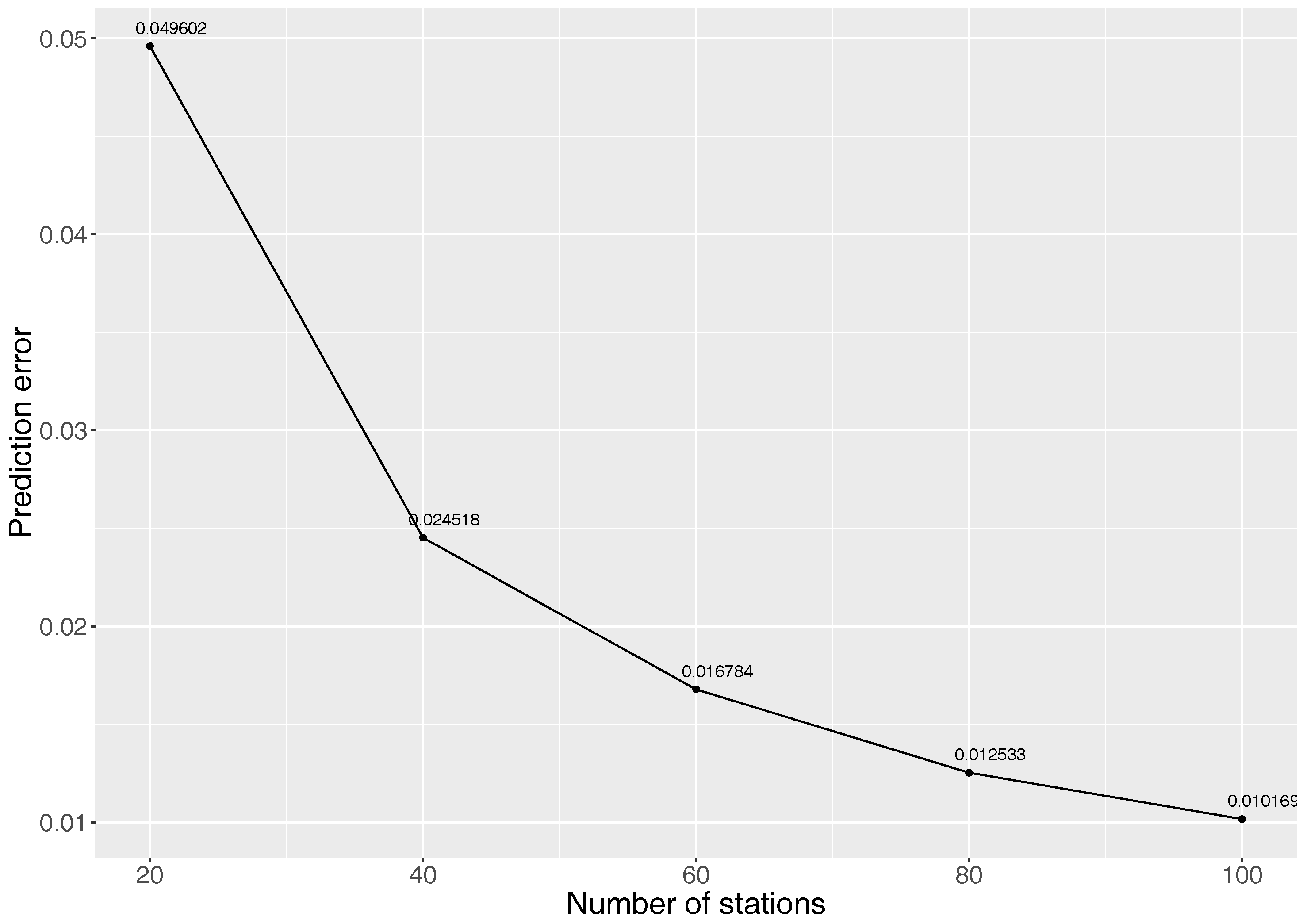
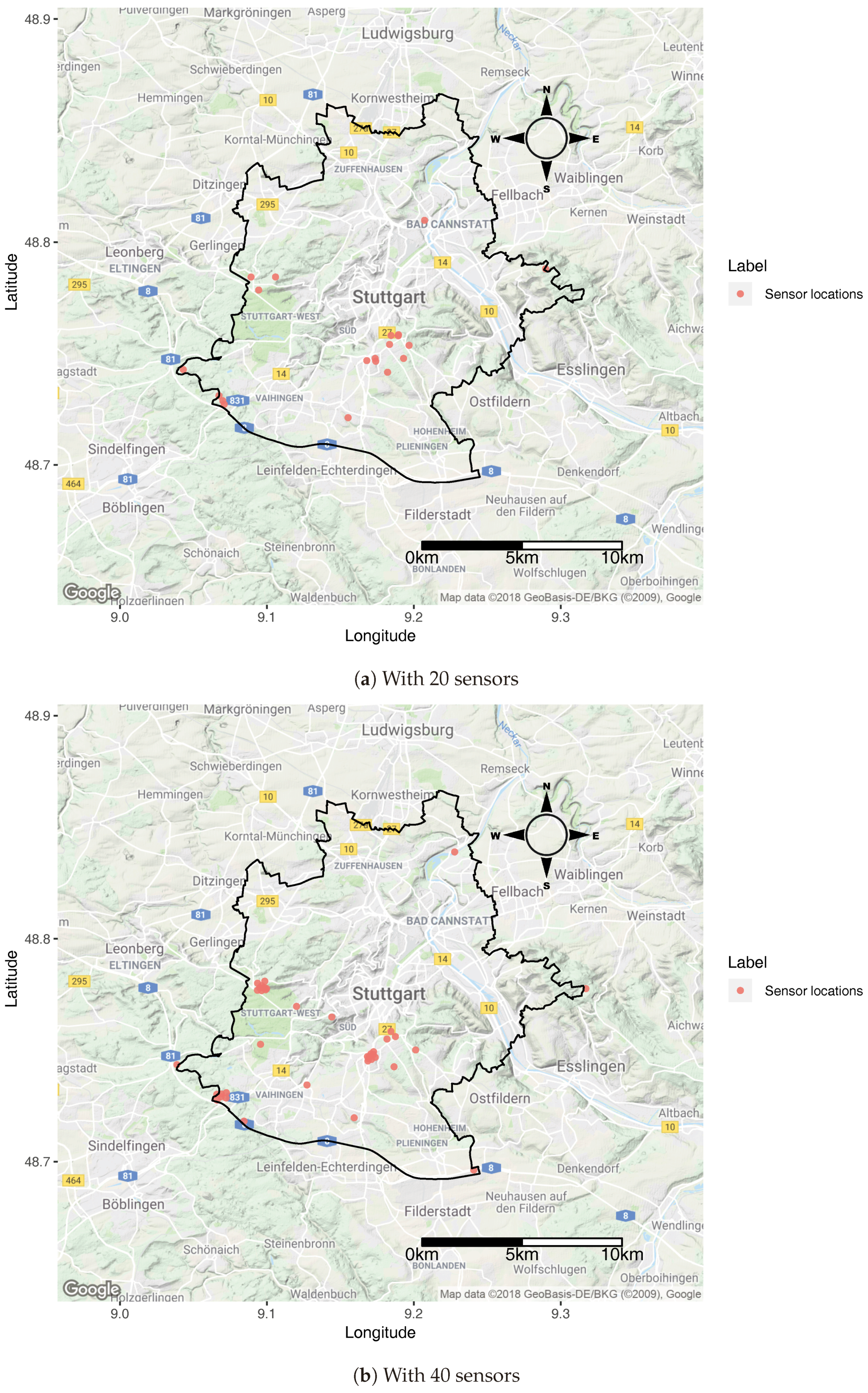
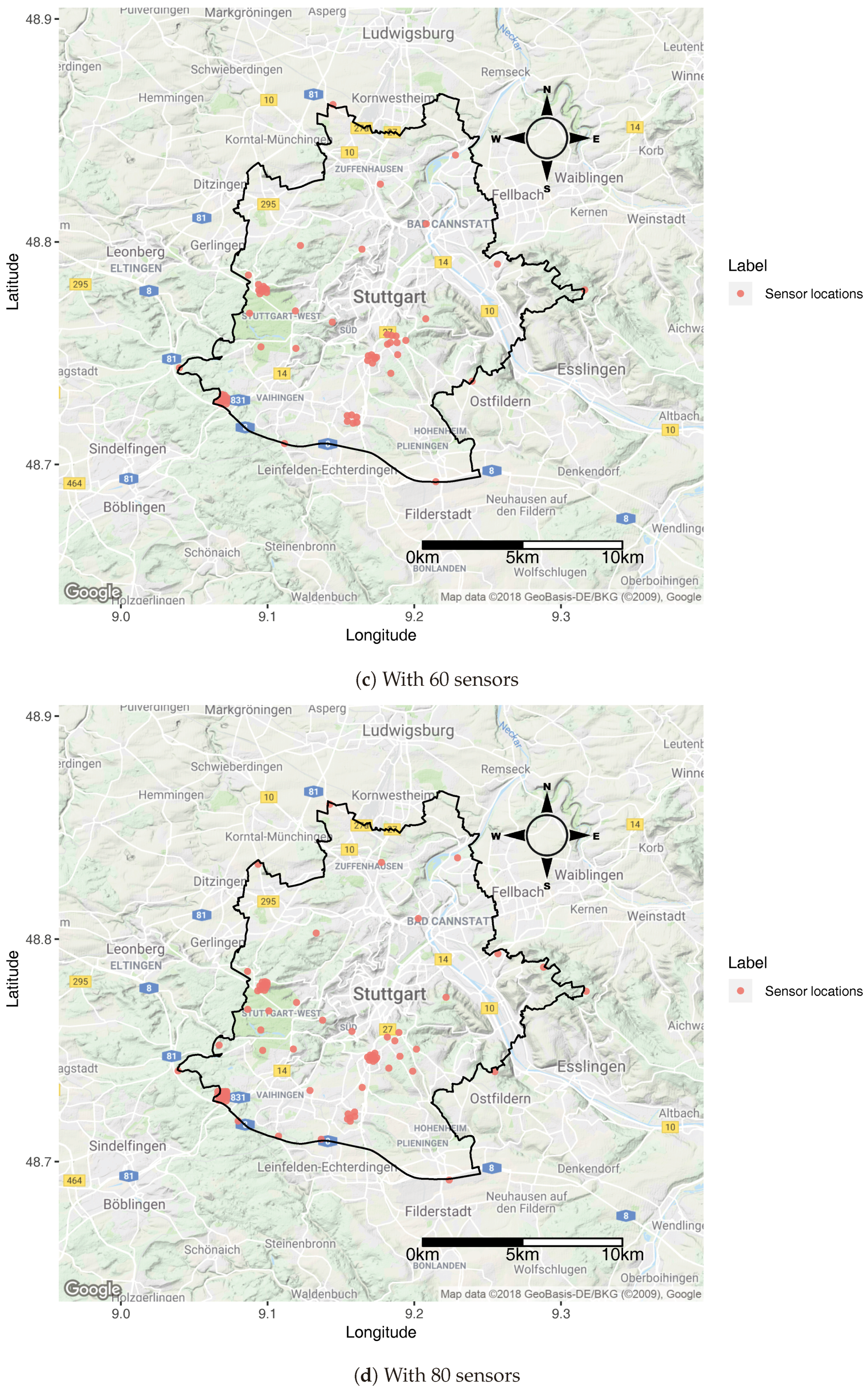
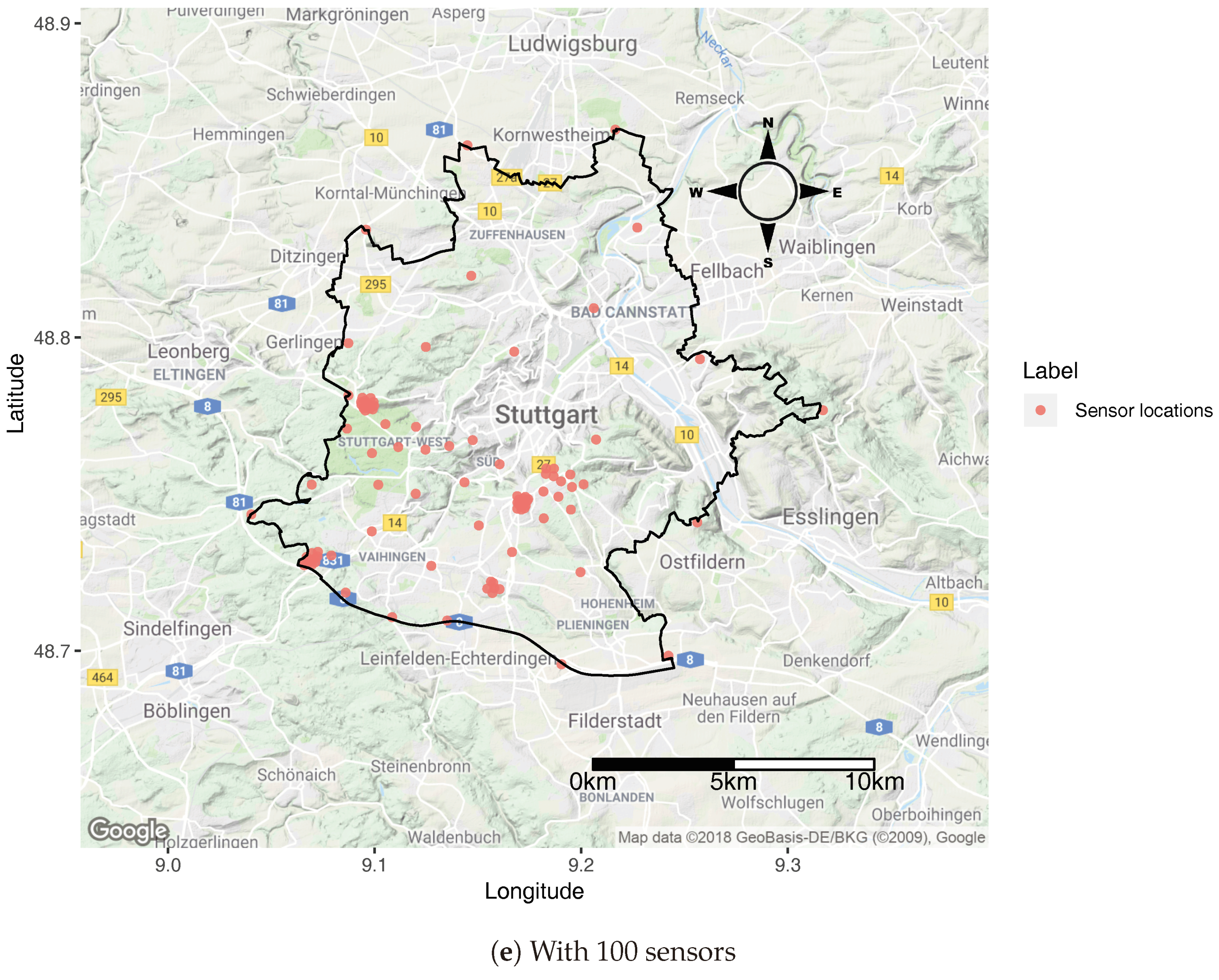
To investigate further the number of sensors required in the monitoring network for deployment in the city, we ran the optimisation process with 20, 40, 60, 80 and 100 sensors. Figure 7 shows the influence of the change in monitoring network size on the prediction error aspect value from the developed optimisation objective function with equal weight on both wide-spread as well as prediction error aspect (i.e., W1 = W2 = 0.5). In the graph, we can note that the deployment of 60 sensors in the study area can already help in monitoring air pollution while decreasing the prediction error aspect substantially. As the figure suggests, different sensor numbers lead to different values for the overall prediction error aspect. The answer to the question “how many sensors should be deployed” is therefore dependent on the wishes of the VGI-campaign organisers as to the final overall prediction error of the collected data. Figure 8 presents various optimal configuration of monitoring network obtained while running the optimisation method with the different number of monitoring station for initiating a VGI campaign.
5.1.2. Location Significance
After understanding the influence of the number of sensors for deployment, another aspect of importance is to know the locations which are significantly important for the overall monitoring network design. Figure 9 presents a collective plot of all the configurations we realised with different number of sensors for optimisation, which can help in inferring the locations of significance in the study area for deploying sensors considering a given LUR model. The optimal locations obtained from various runs of the optimisation method with different numbers of monitoring stations suggests that few of the locations (encircled by red in Figure 9) are key to the minimisation of the LUR model prediction error. The results thus demonstrate the potential of the optimisation method to identify locations which require significant attention and must not be neglected while initiating a new VGI campaign for air pollution data collection.
5.2. Finding Out Where to Place New VGI Sensors
We utilised the LUR model developed from the existing sensor data to test the optimisation method’s ability to find optimal locations using the newly developed LUR (Equation (7)). The quality of the LUR model developed was low ( of 0.1442). Nevertheless, we believe that even with low explanatory power, the developed model was more reliable to represent the air pollution in the study area than an arbitrarily selected model (Section 4.2.1). The explanatory variables of the developed LUR model were then used in the optimisation method for determining optimal locations.
Same as for the previous case, the optimisation method was then run to identify optimal locations. The existing network configuration in Figure 2 was used as the initial configuration for the optimisation process. The resulting configuration (see Appendix B) acknowledged the spread aspect for identifying locations that were widely spread as well as decreased the prediction error aspect from 0.01870 to 0.008903, as a percentage decrease of 52.39%.
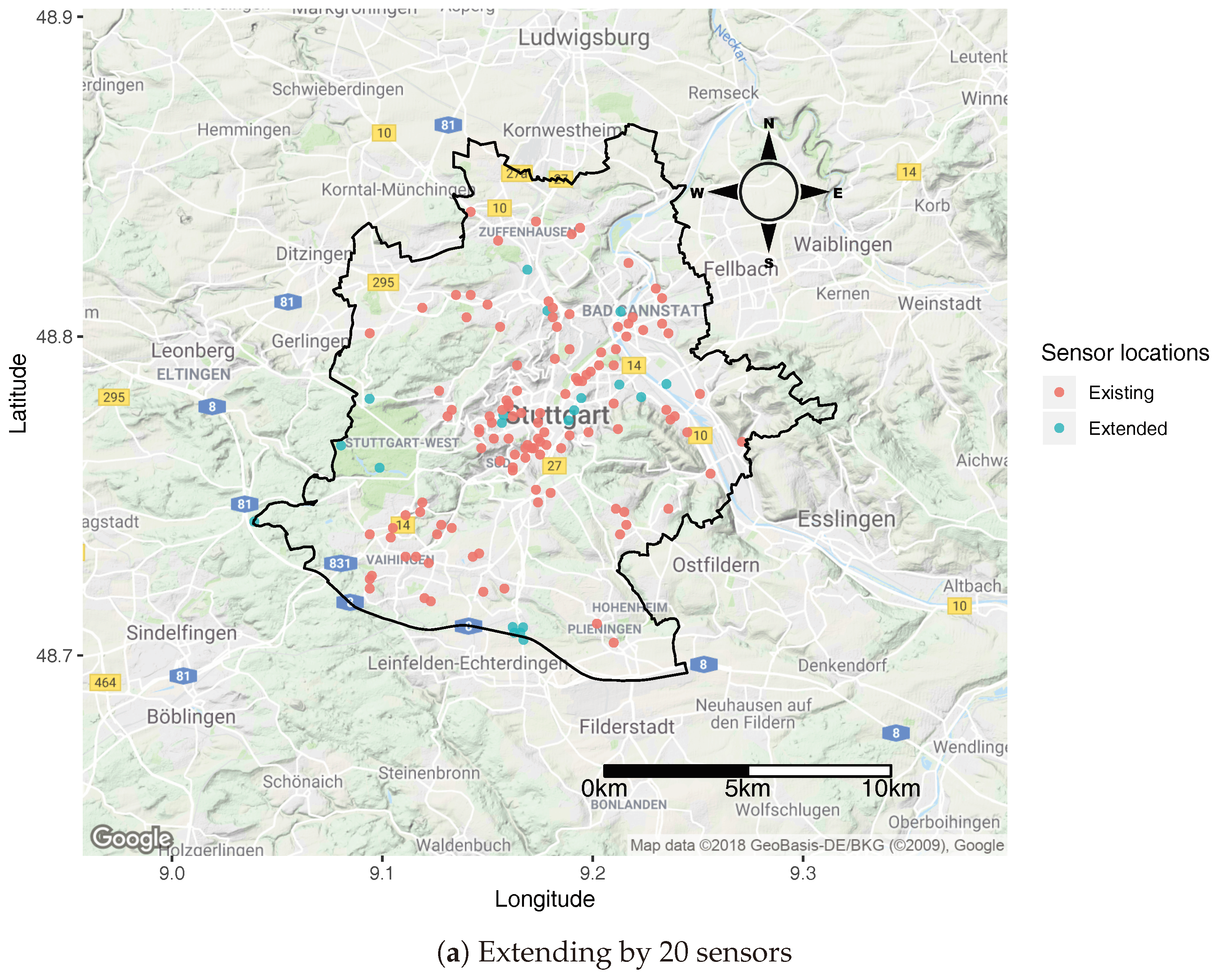
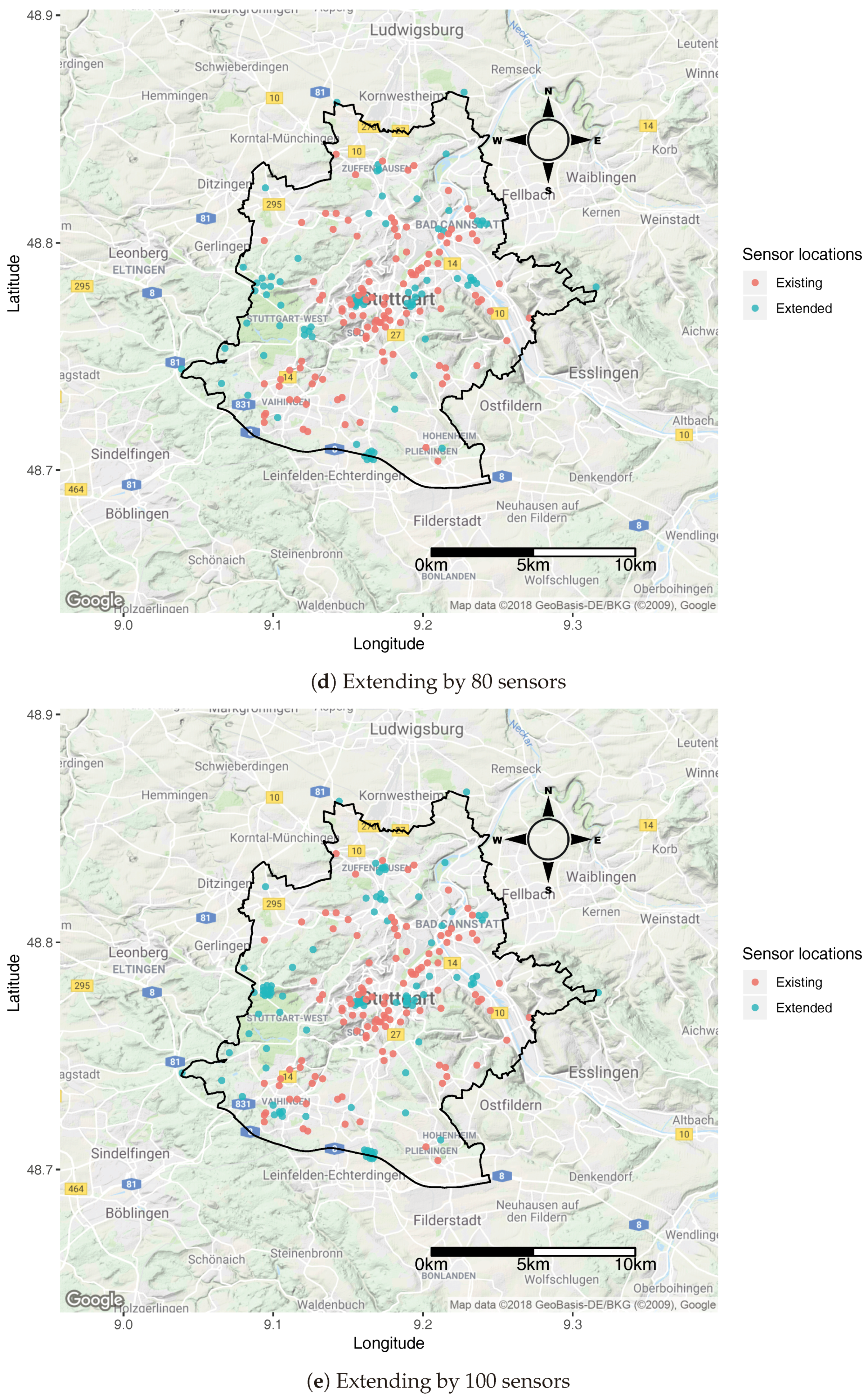
Figure 10 shows the influence on the prediction error when the existing monitoring network in the study area was extended by 20, 40, 60, 80 and 100 sensors. It is apparent in the figure that, with the addition of more monitoring stations systematically, the prediction error decreased. Figure 11 presents various monitoring network configurations realised during the expansion of the existing monitoring network by adding the few certain number of sensors. The optimal locations identified in the optimisation process can be used for further extending the existing VGI sensor network.
6. Discussion
This section reflects on the significance of the study as well as its limitations, and points at future work.
6.1. Significance
The study demonstrates the application of the optimisation method which can aid in the systematic deployment of low-cost sensors for detailed air quality monitoring while considering the scientific models such as LUR. Low-cost sensors can provide data with very high spatial and temporal resolution, which is not feasible with conventional measurement approaches. The study provided means to combine low-sensor datasets to a scientifically recognised air pollution modelling approach to facilitate a better air pollution data collection in the city. The developed optimisation method builds upon ideas suggested by Gupta et al. [27], to optimise air quality monitoring networks for VGI campaigns. The significant performance of the proposed optimisation method to decrease the mean prediction error by 52% along with wide-spread sensor network, demonstrate its applicability to enable systematic planning for (purposeful) VGI campaigns for air pollution monitoring.
The wide-spread VGI campaign sources can be useful for overcoming the issues connected to data quality, such as field duplication, data duplication and irregular spread of sensors, as pointed out by Clements et al. [22] and Budde et al. [37]. The optimisation method also helps answer the research question that need to be considered for planning deployment of sensor network (LUR in our case) to drive the data collection process. By defining the objectives before data collection, the method can be useful for reducing the cost of deployment by limiting the number of sensor nodes required. The method can also be beneficial to identify locations which are easily accessible for sensor maintenance and calibration, for example by using population-weighted optimisation [27]. Such extensions can assist in decreasing sensor failure and replacement costs for successful long-term deployment. If the population weights are considered, the optimisation method can foster construction of LUR models with network design incorporating area close to population and roads, which can better characterise the full range of pollutant concentrations close to population [79].
Since the currently available sophisticated monitoring stations are not capable of expressing the air pollution variability at a detailed spatial scale, the wide-spread and lower prediction error based low-cost monitoring network can be an alternative for gathering measurements, which can be detailed and informative. Using alternative data sources also helps in overcoming the sparsity and scarcity challenges existing in the literature. The resilience of the developed optimisation objective function to prioritise the wide-spread and prediction-error aspect could be advantageous for developing a systematic crowdsourcing sensor network whose measurements can be used in versatile air quality modelling approaches. The spatial spread aspect of the proposed optimisation method helps in shrinking the effects caused by spatial correlation in LUR residuals (which usually exist, see Beelen et al. [80]). However, using weighted least squares (WLS) instead of ordinary least square (OLS) for Equation (3) or considering the kriging prediction error based optimisation as suggested by van Groenigen [67] would have presented an analogous effect on the spatial spread of optimal configuration as the spread aspect of the proposed optimisation objective function achieved for declustering points. The method also inherits the flexibility offered by LUR and SSA, making it more implementable even in cases where availability of data is limited. The outcome of the optimisation objective function considering the wide-spread distribution aspect can also help in distributing the points in different land use type, which can be constructive for developing robust LUR models as suggested by Wu et al. [79].
The current state of sensor technologies with relatively large measurement uncertainties lead to concerns regarding engaging the citizens in the data collection process. Observing spikes while collecting data using VGI approaches may promote behavioural change which can help in preventing exposure to bad air quality. On the other side, this may also lead to panic situations, possibly negating any health benefit. Nevertheless, relating the spikes to the geographical variables such as road counts, traffic, and other emission sources by using LUR models may help to better inform citizens about their actions and local area contributions. Furthermore, the low-cost sensors data might not be monetised for proper air quality applications, but the LUR approach used in the study can act as a tool to process and visualise the data; the resulting analysis and the corresponding information generated can be easily monetised.
Overall, the optimisation method can help in defining the locations for systematic VGI campaign planning, which anticipates the wise use of the participation efforts along with reducing the error for air pollution modelling. The use of open and easily accessible data for VGI campaign systematic deployment, make this approach more implementable. Another major benefit of deploying VGI sensors is their ability to measure real-time data and provide immediate feedback that helps in improving the air pollution monitoring strategy systematically with the help of the proposed optimisation method. This also gives the opportunity to serve as a tool to help in building the capacity of participants to understand air pollution and the influence of geographical variables in the proximity, which can also explain air pollutant’s variability. The wide-spread distribution aspect in the proposed optimisation method could also help to identify potential sources of air pollution otherwise unknown to regulatory authorities.
6.2. Limitation and Outlook
Along with the advantages, the proposed optimisation method also brings some challenges and limitations. One of the critical limitations for the application of the low-cost sensor data for air pollution monitoring is the reliability of the measured data. Further challenges include short working time and calibration challenge [22]. In the study, the quality of the LUR model developed was low ( = 0.1442) which may be due to the quality of data produced by the low-cost devices, and the locations from where they were collected [79]. Developing new LUR models using inputs from improved VGI sensors could help better estimate the impact of sensor type on LUR model estimations.
In addition to these limitations related to the use of low-cost sensor data, there are limitations concerning the proposed optimisation method. To begin with, the selection of LUR model is the first step to find the optimal location, which means that, if we do not have a LUR model for the study area, we have to select one from the previous studies by specifying some assumption based rules for model selection. The selection of a LUR model based on some assumptions may not involve variables that are convincing enough to explain air pollution in the study area. Another limitation of the approach concerns the use of a LUR model and the underlying assumptions of multiple linear regression (e.g., linearity between dependent and independent variables, independent and normal distribution of error terms may create biases in interpreting the outcomes, which are the typical limitations for any simplistic regression-based studies). Limitations also exist for the SSA approach; as it is a stochastic method, every different run of optimisation method may yield different monitoring network designs. The process of optimisation is also very time-consuming, depending on the input parameters of annealing, variables used for computing the objective function and the study area size. While running the optimisation for the study, the process took 6–8 h for one optimisation outcome.
As can be seen from the results, the output of the optimisation ended up being clustered. This clustering can sometimes be caused by the spatial auto-correlation of the predictor variables, which lead to all points being close to each other. The reliability of the LUR used for the optimisation may also contribute to the clustered results. Devising the methods that address these limitations by taking into account robust LUR, and information on the spatial correlation and interpolation based constraints can be helpful in improving the design objectives of the study. We have not considered such factors in our study but future work could consider integrating it. It would also be interesting to investigate a combination of our method and active learning (see [81]) for the purpose of optimal air quality network monitoring (e.g., our method helps to identify key locations during the monitoring process, and these could inform the labelling phase of an active learning approach). Extending the developed optimisation method to consider the population distribution weights proposed by Gupta et al. [27] can also be useful in identifying the locations close to living spaces. A population-based weight can be useful in two ways. Firstly, identifying locations where the citizens live can make the initiation of VGI campaign easier. Secondly, it promotes the gathering of air pollution data that represent the real exposure of the population in the living spaces of the city. For the practical implementation of the proposed optimisation method for VGI approaches, future work can focus on integrating the optimal location identification method with citizen observatory based projects (e.g., FLAMENCO Project [82]). Integration with citizen observatory based projects can be fruitful because the optimisation method can identify the locations and citizen observatory can identify the participants at the optimal location, making the overall flow of VGI-campaign initiation easy.
As discussed in previous studies related to low-cost sensors deployment [22,37], the field of low-cost sensors for environmental monitoring is in transition, and more work is needed to continue exploring the potential of low-cost sensors for air pollution monitoring. With the help of low-cost sensor systematic deployment initiatives by using citizen participation approaches, it is possible to bring forward a whole new system which anticipates the development of open data platforms (e.g., OK Labs [60]). These initiatives also help in connecting other systems that utilise air quality data such as health informatics, housing companies, and sustainable urban planning, thereby helping in enabling the development of tools and techniques that can improve Quality of Life (QoL) in cities.
7. Conclusions
In this paper, we propose an optimisation method that can help in the systematic deployment of air pollution monitoring sensors for VGI approaches. A systematic deployment of monitoring stations in the city is desirable to enable air pollution monitoring with higher accuracy. The optimisation method suggested takes into account two important aspects, namely, the decreasing of a given LUR model’s prediction error and the wide-spread distribution of locations in the study area. The decreased prediction error aspect can help in developing more robust LUR models, and the wide-spread distribution aspect supports in making the data collection approach more versatile and informative. The applicability of the optimisation method was demonstrated using two practical test cases: (1.) initiating a new VGI campaign, and (2.) placing new VGI sensors. In the first test case, the optimisation method identifies the set of locations using explanatory variables of an already existing LUR model. This approach is used to initiate a VGI campaign for the cities where no air pollution data is available to develop the LUR model. In the second test case, a LUR model was developed using the VGI based air pollution data source. The results of the optimisation method revealed a significant decrease in prediction error (by 52%) while taking into account the wide-spread distribution. The method can thus be potentially useful to policymakers for the systematic planning of the size and location of VGI campaigns. The availability of more accurate and open data, improved low-cost sensor for reliability and systematic deployment of sensors in VGI campaign may help in refining the performance of the proposed optimisation method for more robust results. Future work can also involve integrating the optimisation method with citizen science observatories to identify participants at the optimal locations identified by the objective function.
Author Contributions
The contributions of the respective authors are as follows: S.G. and A.D. conceived and designed the study; S.G. performed the analysis; E.P. supervised the research; and S.G. wrote a draft of the manuscript, which was iteratively improved by all other authors of the manuscript.
Funding
The authors gratefully acknowledge funding from the European Union through the GEO-C project (H2020-MSCA-ITN-2014, Grant Agreement Number 642332, http://www.geo-c.eu/).
Conflicts of Interest
The authors declare no conflict of interest.
Abbreviations
The following abbreviations are used in this manuscript:
| ESCAPE | European study of cohorts for air pollution effects |
| IMSD | Inverse mean shortest distance |
| LUR | Land Use Regression |
| OLS | Ordinary Least Squares |
| Particulate matter (PM) that have a diameter of less than 2.5 micrometers | |
| QoL | Quality of Life |
| SQRALT | Square root of altitude |
| SSA | Spatial Simulated Annealing |
| USEPA | United States Environmental Protection Agency |
| VGI | Volunteered Geographic Information |
| WHO | World Health Organisation |
| WLS | Weighted Least square |
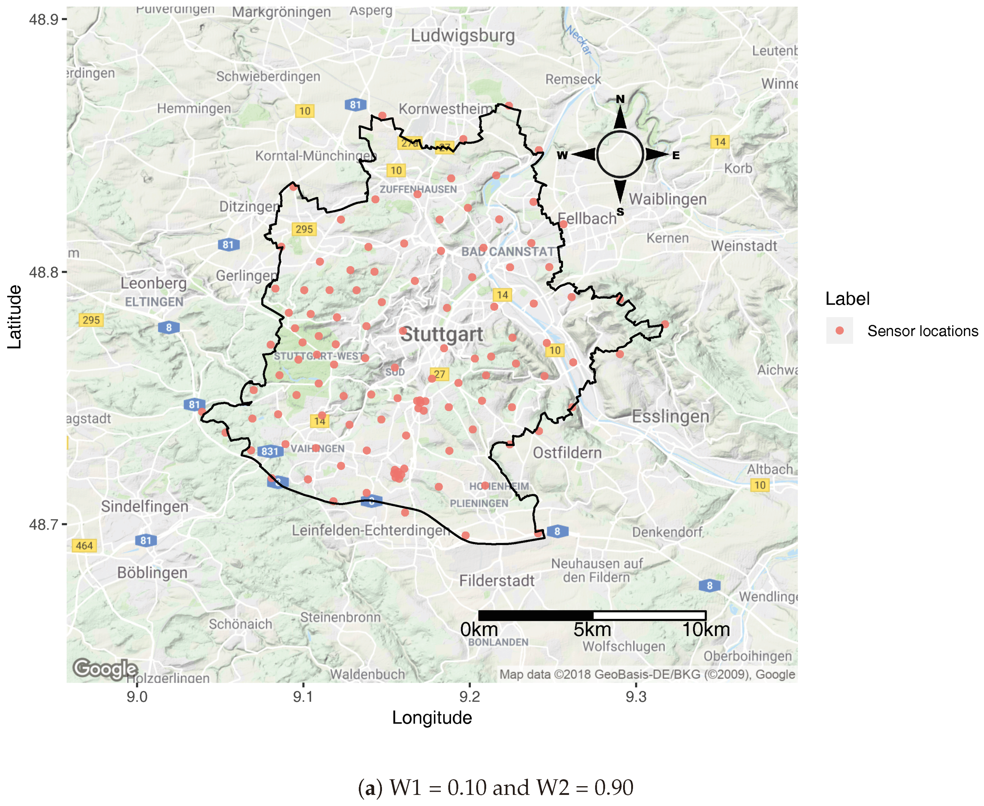
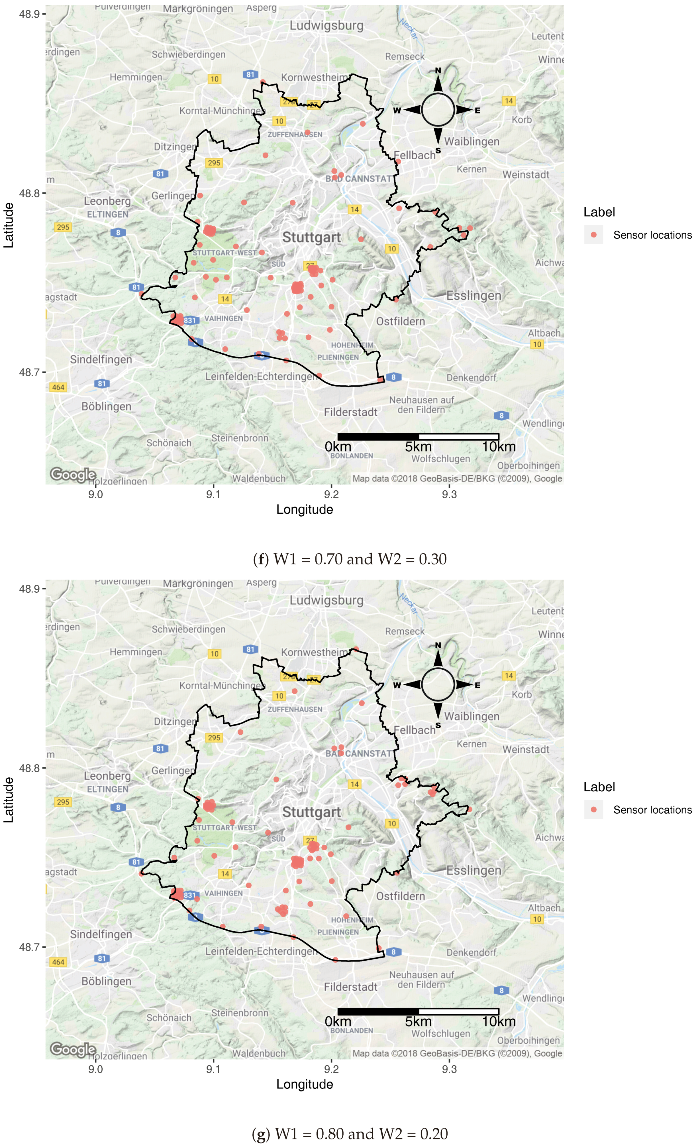
Appendix A
Figure A1.
Configuration with various weights on prediction error (W1) and wide-spread (W2) aspect of developed objective function.
Figure A1.
Configuration with various weights on prediction error (W1) and wide-spread (W2) aspect of developed objective function.


Appendix B
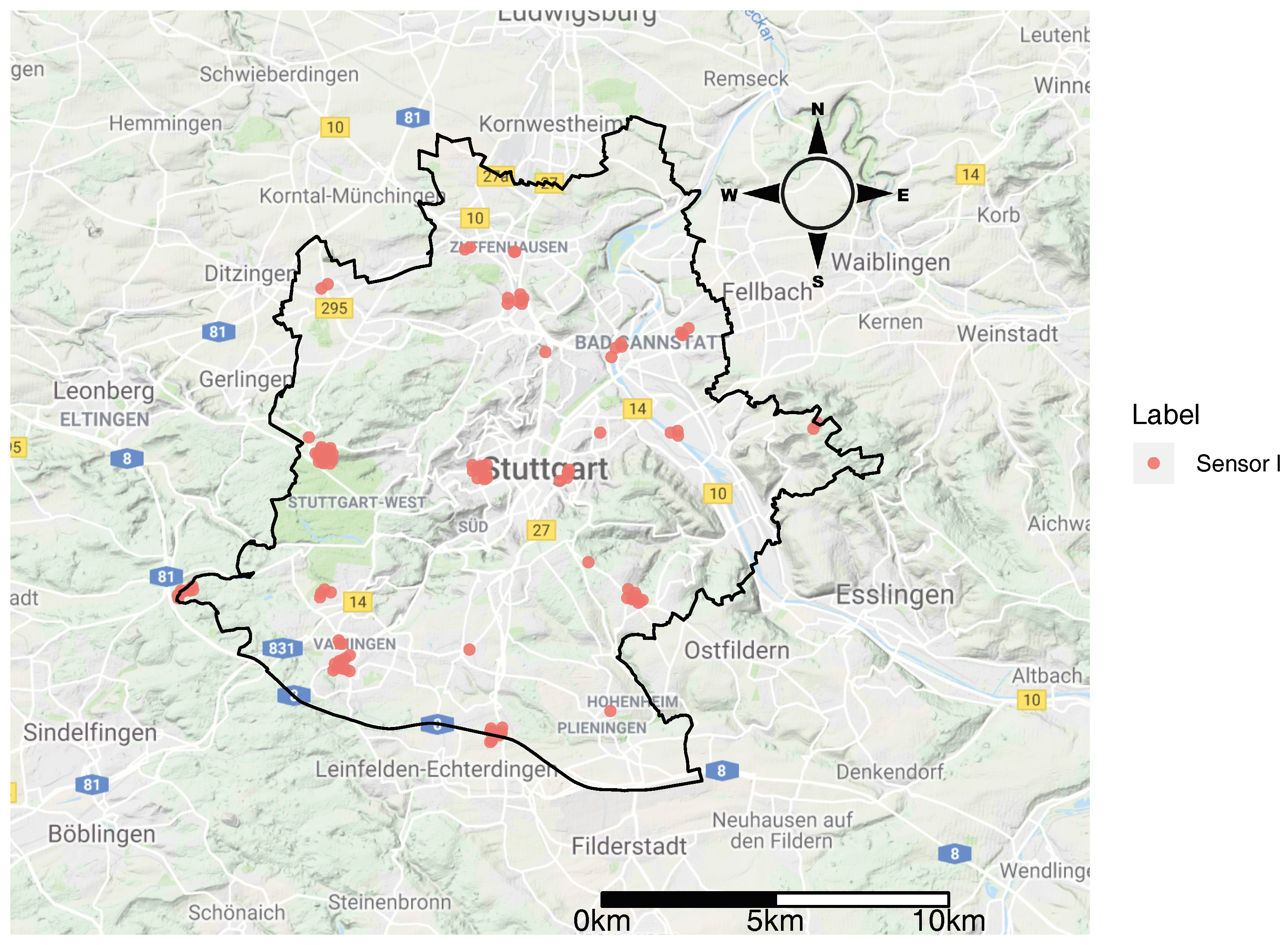
Figure A2.
Optimal locations considering prediction error constraint for Stuttgart LUR model developed using low-cost sensor network data.
Figure A2.
Optimal locations considering prediction error constraint for Stuttgart LUR model developed using low-cost sensor network data.

Figure A3.
Optimal locations considering prediction error and wide-spread aspect in the objective function for Stuttgart LUR model developed using low-cost sensor network data.
Figure A3.
Optimal locations considering prediction error and wide-spread aspect in the objective function for Stuttgart LUR model developed using low-cost sensor network data.

References
- Molina, L.T.; Molina, M.J.; Slott, R.S.; Kolb, C.E.; Gbor, P.K.; Meng, F.; Singh, R.B.; Galvez, O.; Sloan, J.J.; Anderson, W.P.; et al. Air quality in selected megacities. J. Air Waste Manag. Assoc. 2004, 54, 1–73. [Google Scholar] [CrossRef]
- Barer, M. Why Are Some People Healthy and Others Not? Routledge: Abingdon, UK, 2017. [Google Scholar]
- Brown, J.; Bowman, C. Integrated Science Assessment for Ozone and Related Photochemical Oxidants; US Environmental Protection Agency: Washington, DC, USA, 2013.
- Bauernschuster, S.; Hener, T.; Rainer, H. When labor disputes bring cities to a standstill: The impact of public transit strikes on traffic, accidents, air pollution, and health. Am. Econ. J. Econ. Policy 2017, 9, 1–37. [Google Scholar] [CrossRef]
- WHO. WHO Releases Country Estimates on Air Pollution Exposure and Health Impact; WHO: Geneva, Switzerland, 2016. [Google Scholar]
- Jerrett, M.; Arain, M.A.; Kanaroglou, P.; Beckerman, B.; Crouse, D.; Gilbert, N.L.; Brook, J.R.; Finkelstein, N.; Finkelstein, M.M. Modeling the intraurban variability of ambient traffic pollution in Toronto, Canada. J. Toxicol. Environ. Health Part A 2007, 70, 200–212. [Google Scholar] [CrossRef] [PubMed]
- Hamra, G.B.; Laden, F.; Cohen, A.J.; Raaschou-Nielsen, O.; Brauer, M.; Loomis, D. Lung cancer and exposure to nitrogen dioxide and traffic: A systematic review and meta-analysis. Environ. Health Perspect. 2015, 123, 1107. [Google Scholar] [CrossRef] [PubMed]
- Khreis, H.; Kelly, C.; Tate, J.; Parslow, R.; Lucas, K.; Nieuwenhuijsen, M. Exposure to traffic-related air pollution and risk of development of childhood asthma: A systematic review and meta-analysis. Environ. Int. 2017, 100, 1–31. [Google Scholar] [CrossRef] [PubMed]
- Bauer, K.; Bosker, T.; Dirks, K.N.; Behrens, P. The impact of seating location on black carbon exposure in public transit buses: Implications for vulnerable groups. Transp. Rese. Part D Transp. Environ. 2018, 62, 577–583. [Google Scholar] [CrossRef]
- Conti, G.O.; Heibati, B.; Kloog, I.; Fiore, M.; Ferrante, M. A review of AirQ Models and their applications for forecasting the air pollution health outcomes. Environ. Sci. Pollut. Res. 2017, 24, 6426–6445. [Google Scholar] [CrossRef] [PubMed]
- Mayer, H. Air pollution in cities. Atmos. Environ. 1999, 33, 4029–4037. [Google Scholar] [CrossRef]
- Van Nunen, E.; Vermeulen, R.; Tsai, M.Y.; Probst-Hensch, N.; Ineichen, A.; Davey, M.; Imboden, M.; Ducret-Stich, R.; Naccarati, A.; Raffaele, D.; et al. Land use regression models for ultrafine particles in six European areas. Environ. Sci. Technol. 2017, 51, 3336–3345. [Google Scholar] [CrossRef] [PubMed]
- Wolf, K.; Cyrys, J.; Harciníková, T.; Gu, J.; Kusch, T.; Hampel, R.; Schneider, A.; Peters, A. Land use regression modeling of ultrafine particles, ozone, nitrogen oxides and markers of particulate matter pollution in Augsburg, Germany. Sci. Total Environ. 2017, 579, 1531–1540. [Google Scholar] [CrossRef] [PubMed]
- Weichenthal, S.; Van Ryswyk, K.; Goldstein, A.; Bagg, S.; Shekkarizfard, M.; Hatzopoulou, M. A land use regression model for ambient ultrafine particles in Montreal, Canada: A comparison of linear regression and a machine learning approach. Environ. Res. 2016, 146, 65–72. [Google Scholar] [CrossRef] [PubMed] [Green Version]
- Jiao, W.; Hagler, G.; Williams, R.; Sharpe, R.; Brown, R.; Garver, D.; Judge, R.; Caudill, M.; Rickard, J.; Davis, M.; et al. Community Air Sensor Network (CAIRSENSE) project: Evaluation of low-cost sensor performance in a suburban environment in the southeastern United States. Atmos. Meas. Tech. 2016, 9, 5281–5292. [Google Scholar] [CrossRef]
- Snyder, E.G.; Watkins, T.H.; Solomon, P.A.; Thoma, E.D.; Williams, R.W.; Hagler, G.S.; Shelow, D.; Hindin, D.A.; Kilaru, V.J.; Preuss, P.W. The Changing Paradigm of Air Pollution Monitoring; ACS Publications: Washington, DC, USA, 2013. [Google Scholar]
- Yi, W.Y.; Lo, K.M.; Mak, T.; Leung, K.S.; Leung, Y.; Meng, M.L. A survey of wireless sensor network based air pollution monitoring systems. Sensors 2015, 15, 31392–31427. [Google Scholar] [CrossRef] [PubMed]
- Shusterman, A.A.; Teige, V.E.; Turner, A.J.; Newman, C.; Kim, J.; Cohen, R.C. The BErkeley Atmospheric CO2 Observation Network: Initial evaluation. Atmos. Chem. Phys. 2016, 16, 13449–13463. [Google Scholar] [CrossRef]
- Fang, X.; Bate, I. Issues of using wireless sensor network to monitor urban air quality. In Proceedings of the First ACM International Workshop on the Engineering of Reliable, Robust, and Secure Embedded Wireless Sensing Systems, Delft, The Netherlands, 6–8 November 2017; pp. 32–39. [Google Scholar]
- Castell, N.; Dauge, F.R.; Schneider, P.; Vogt, M.; Lerner, U.; Fishbain, B.; Broday, D.; Bartonova, A. Can commercial low-cost sensor platforms contribute to air quality monitoring and exposure estimates? Environ. Int. 2017, 99, 293–302. [Google Scholar] [CrossRef] [PubMed]
- Schneider, P.; Castell, N.; Vogt, M.; Dauge, F.R.; Lahoz, W.A.; Bartonova, A. Mapping urban air quality in near real-time using observations from low-cost sensors and model information. Environ. Int. 2017, 106, 234–247. [Google Scholar] [CrossRef] [PubMed]
- Clements, A.L.; Griswold, W.G.; Rs, A.; Johnston, J.E.; Herting, M.M.; Thorson, J.; Collier-Oxandale, A.; Hannigan, M. Low-cost air quality monitoring tools: from research to practice (a workshop summary). Sensors 2017, 17, 2478. [Google Scholar] [CrossRef] [PubMed]
- Watkins, T. DRAFT Roadmap for Next Generation Air Monitoring; Environmental Protection Agency: Washington, DC, USA, 2013.
- Kanaroglou, P.S.; Jerrett, M.; Morrison, J.; Beckerman, B.; Arain, M.A.; Gilbert, N.L.; Brook, J.R. Establishing an air pollution monitoring network for intra-urban population exposure assessment: A location-allocation approach. Atmos. Environ. 2005, 39, 2399–2409. [Google Scholar] [CrossRef]
- Bonney, R.; Shirk, J.L.; Phillips, T.B.; Wiggins, A.; Ballard, H.L.; Miller-Rushing, A.J.; Parrish, J.K. Next steps for citizen science. Science 2014, 343, 1436–1437. [Google Scholar] [CrossRef] [PubMed]
- Elwood, S.; Goodchild, M.F.; Sui, D.Z. Researching volunteered geographic information: Spatial data, geographic research, and new social practice. Ann. Assoc. Am. Geogr. 2012, 102, 571–590. [Google Scholar] [CrossRef]
- Gupta, S.; Pebesma, E.; Mateu, J.; Degbelo, A. Air Quality Monitoring Network Design Optimisation for Robust Land Use Regression Models. Sustainability 2018, 10, 1442. [Google Scholar] [CrossRef]
- Goodchild, M.F.; Li, L. Assuring the quality of volunteered geographic information. Spat. Stat. 2012, 1, 110–120. [Google Scholar] [CrossRef]
- Sieber, R.E.; Haklay, M. The epistemology(s) of volunteered geographic information: A critique. Geo Geogr. Environ. 2015, 2, 122–136. [Google Scholar] [CrossRef]
- Senaratne, H.; Mobasheri, A.; Ali, A.L.; Capineri, C.; Haklay, M.M. A review of volunteered geographic information quality assessment methods. Int. J. Geogr. Inf. Sci. 2017, 31, 139–167. [Google Scholar] [CrossRef]
- Haklay, M. How good is volunteered geographical information? A comparative study of OpenStreetMap and Ordnance Survey datasets. Environ. Plan. B Plan. Des. 2010, 37, 682–703. [Google Scholar] [CrossRef]
- Jackson, S.; Mullen, W.; Agouris, P.; Crooks, A.; Croitoru, A.; Stefanidis, A. Assessing completeness and spatial error of features in volunteered geographic information. ISPRS Int. J. Geo-Inf. 2013, 2, 507–530. [Google Scholar] [CrossRef]
- Gupta, S.; Pebesma, E.; Mateu, J.; Degbelo, A. Connecting Citizens and Housing Companies for Fine-grained Air Quality Sensing. GI_Forum J. Geogr. Inf. Sci. 2018, in press. [Google Scholar]
- Gabrys, J.; Pritchard, H. Just Good Enough Data and Environmental Sensing: Moving Beyond Regulatory Benchmarks toward Citizen Action. Int. J. Spat. Data Infrastruct. Res. 2018, 13, 4–14. [Google Scholar]
- Jovašević-Stojanović, M.; Bartonova, A.; Topalović, D.; Lazović, I.; Pokrić, B.; Ristovski, Z. On the use of small and cheaper sensors and devices for indicative citizen-based monitoring of respirable particulate matter. Environ. Pollut. 2015, 206, 696–704. [Google Scholar] [CrossRef] [PubMed]
- Lisjak, J.; Schade, S.; Kotsev, A. Closing data gaps with citizen science? Findings from the Danube region. ISPRS Int. J. Geo-Inf. 2017, 6, 277. [Google Scholar] [CrossRef]
- Budde, M.; Schankin, A.; Hoffmann, J.; Danz, M.; Riedel, T.; Beigl, M. Participatory Sensing or Participatory Nonsense?: Mitigating the Effect of Human Error on Data Quality in Citizen Science. IMWUT 2017, 1, 39. [Google Scholar] [CrossRef]
- Hoek, G.; Beelen, R.; De Hoogh, K.; Vienneau, D.; Gulliver, J.; Fischer, P.; Briggs, D. A review of land-use regression models to assess spatial variation of outdoor air pollution. Atmos. Environ. 2008, 42, 7561–7578. [Google Scholar] [CrossRef]
- Wang, M.; Beelen, R.; Eeftens, M.; Meliefste, K.; Hoek, G.; Brunekreef, B. Systematic evaluation of land use regression models for NO2. Environ. Sci. Technol. 2012, 46, 4481–4489. [Google Scholar] [CrossRef] [PubMed]
- Basagaña, X.; Rivera, M.; Aguilera, I.; Agis, D.; Bouso, L.; Elosua, R.; Foraster, M.; de Nazelle, A.; Nieuwenhuijsen, M.; Vila, J.; et al. Effect of the number of measurement sites on land use regression models in estimating local air pollution. Atmos. Environ. 2012, 54, 634–642. [Google Scholar] [CrossRef]
- Hystad, P.; Setton, E.; Cervantes, A.; Poplawski, K.; Deschenes, S.; Brauer, M.; van Donkelaar, A.; Lamsal, L.; Martin, R.; Jerrett, M.; et al. Creating national air pollution models for population exposure assessment in Canada. Environ. Health Perspect. 2011, 119, 1123. [Google Scholar] [CrossRef] [PubMed]
- Jerrett, M.; Arain, A.; Kanaroglou, P.; Beckerman, B.; Potoglou, D.; Sahsuvaroglu, T.; Morrison, J.; Giovis, C. A review and evaluation of intraurban air pollution exposure models. J. Expo. Sci. Environ. Epidemiol. 2005, 15, 185. [Google Scholar] [CrossRef] [PubMed]
- Peng, J.; Hu, M.; Wang, Z.; Huang, X.; Kumar, P.; Wu, Z.; Guo, S.; Yue, D.; Shang, D.; Zheng, Z.; et al. Submicron aerosols at thirteen diversified sites in China: size distribution, new particle formation and corresponding contribution to cloud condensation nuclei production. Atmos. Chem. Phys. 2014, 14, 10249–10265. [Google Scholar] [CrossRef] [Green Version]
- Official Journal of the European Union. Directive 2008/50/EC of the European Parliament and of the Council of 21 May 2008 on Ambient Air Quality and Cleaner Air for Europe; Official Journal of the European Union: Brussels, Belgium, 2008. [Google Scholar]
- Goldstein, I.F.; Landovitz, L. Analysis of air pollution patterns in New York City—I. Can one station represent the large metropolitan area? Atmos. Environ. 1977, 11, 47–52. [Google Scholar] [CrossRef]
- Ott, D.K.; Kumar, N.; Peters, T.M. Passive sampling to capture spatial variability in PM10–2.5. Atmos. Environ. 2008, 42, 746–756. [Google Scholar] [CrossRef]
- Chong, C.Y.; Kumar, S.P. Sensor networks: Evolution, opportunities, and challenges. Proc. IEEE 2003, 91, 1247–1256. [Google Scholar] [CrossRef] [Green Version]
- Borrego, C.; Costa, A.; Ginja, J.; Amorim, M.; Coutinho, M.; Karatzas, K.; Sioumis, T.; Katsifarakis, N.; Konstantinidis, K.; De Vito, S.; et al. Assessment of air quality microsensors versus reference methods: The EuNetAir joint exercise. Atmos. Environ. 2016, 147, 246–263. [Google Scholar] [CrossRef]
- Spinelle, L.; Gerboles, M.; Villani, M.G.; Aleixandre, M.; Bonavitacola, F. Field calibration of a cluster of low-cost commercially available sensors for air quality monitoring. Part B: NO, CO and CO2. Sens. Actuators B Chem. 2017, 238, 706–715. [Google Scholar] [CrossRef]
- Borrego, C.; Coutinho, M.; Costa, A.M.; Ginja, J.; Ribeiro, C.; Monteiro, A.; Ribeiro, I.; Valente, J.; Amorim, J.; Martins, H.; et al. Challenges for a new air quality directive: The role of monitoring and modelling techniques. Urban Clim. 2015, 14, 328–341. [Google Scholar] [CrossRef]
- Benis, K.Z.; Fatehifar, E.; Shafiei, S.; Nahr, F.K.; Purfarhadi, Y. Design of a sensitive air quality monitoring network using an integrated optimization approach. Stoch. Environ. Res. Risk Assess. 2016, 30, 779–793. [Google Scholar] [CrossRef]
- Weissert, L.; Salmond, J.; Miskell, G.; Alavi-Shoshtari, M.; Grange, S.; Henshaw, G.; Williams, D. Use of a dense monitoring network of low-cost instruments to observe local changes in the diurnal ozone cycles as marine air passes over a geographically isolated urban centre. Sci. Total Environ. 2017, 575, 67–78. [Google Scholar] [CrossRef] [PubMed]
- Kim, J.; Shusterman, A.A.; Lieschke, K.J.; Newman, C.; Cohen, R.C. The berkeley atmospheric CO2 observation network: Field calibration and evaluation of low-cost air quality sensors. Atmos. Meas. Tech. Discuss. 2017. [Google Scholar] [CrossRef]
- Baden-Württemberg, S.L. Bevölkerung und Erwerbstätigkeit. Available online: https://www.statistik-bw.de/Service/Veroeff/Statistische_Berichte/312616001.pdf (accessed on 15 August 2018).
- Deutsche Welle. Stuttgart: Germany’s ‘Beijing’ for Air Pollution? Available online: https://www.dw.com/en/stuttgart-germanys-beijing-for-air-pollution/a-18991064 (accessed on 19 August 2018).
- Deutsche Welle. Germany’s Stuttgart Asks Residents to Leave Car at Home Amid High Air Pollution. Available online: https://www.dw.com/en/germanys-stuttgart-asks-residents-to-leave-car-at-home-amid-high-air-pollution/a-18986437 (accessed on 19 August 2018).
- City of Stuttgart. Measuring Points. Available online: https://www.stadtklima-stuttgart.de/index.php?air_clean_air_plan_measuring_points (accessed on 17 August 2018).
- Umbelt Bundesamt. Current Concentrations of Air Pollutants in Germany. Available online: https://www.umweltbundesamt.de/en/data/current-concentrations-of-air-pollutants-in-germany#/ (accessed on 5 August 2018).
- OK Labs. Measure Air Quality Yourself Nearly Finished With Your Help. Available online: https://luftdaten.info/en/home-en/ (accessed on 12 August 2018).
- OK Labs. Data Archive. Available online: https://archive.luftdaten.info (accessed on 10 August 2018).
- OK Labs. Measurement Accuracy. Available online: https://luftdaten.info/messgenauigkeit/ (accessed on 11 August 2018).
- Geofabrik GmbH Karlsruhe. Downloads. Available online: https://www.geofabrik.de/data/download.html (accessed on 19 August 2018).
- OpenStreetMap Contributors. Planet Dump Retrieved from https://planet.osm.org. Available online: https://www.openstreetmap.org (accessed on 19 August 2018).
- Open.NRW. NRW: Zensusatlas 2011—Bundesweite. Available online: https://www.europeandataportal.eu/data/en/dataset/https-ckan-govdata-de-dataset-fe865d7e-90ff-508b-92b5-92819a8f6d2b (accessed on 19 August 2018).
- Bundesamt für Kartographie und Geodäsie. Open Data—Freie Daten und Dienste des BKG. Available online: http://www.geodatenzentrum.de/geodaten/gdz_rahmen.gdz_div?gdz_spr=deu&gdz_akt_zeile=5&gdz_anz_zeile=1&gdz_unt_zeile=0&gdz_user_id=0 (accessed on 9 August 2018).
- Copernicus. CORINE Land Cover. Available online: https://land.copernicus.eu/pan-european/corine-land-cover (accessed on 17 August 2018).
- Van Groenigen, J.W. Constrained Optimisation of Spatial Sampling: A Geostatistical Approach; ITC Publication: Enschede, The Netherlands, 1999. [Google Scholar]
- Heuvelink, G.B.M.; Jiang, Z.; De Bruin, S.; Twenhöfel, C.J.W. Optimization of mobile radioactivity monitoring networks. Int. J. Geogr. Inf. Sci. 2010, 24, 365–382. [Google Scholar] [CrossRef] [Green Version]
- Draper, N.R.; Smith, H. Applied Regression Analysis; John Wiley & Sons: Hoboken, NJ, USA, 2014; Volume 326. [Google Scholar]
- Mitchell, G.; Dorling, D. An environmental justice analysis of British air quality. Environ. Plan. A 2003, 35, 909–929. [Google Scholar] [CrossRef]
- Kumar, P.; Morawska, L.; Martani, C.; Biskos, G.; Neophytou, M.; Di Sabatino, S.; Bell, M.; Norford, L.; Britter, R. The rise of low-cost sensing for managing air pollution in cities. Environ. Int. 2015, 75, 199–205. [Google Scholar] [CrossRef] [PubMed] [Green Version]
- Team, R.C. R: A Language and Environment for Statistical Computing; R Foundation for Statistical Computing: Vienna, Austria, 2017. [Google Scholar]
- Pebesma, E.; Bivand, R.S. Classes and Methods for Spatial Data in R: The sp Package. R News 2005, 5, 9–13. [Google Scholar]
- Pebesma, E. sf: Simple Features for R. R Package Version 0.5-5. 2018. Available online: https://CRAN.R-project.org/package=sf (accessed on 10 June 2018).
- French, J. SpatialTools: Tools for Spatial Data Analysis, R Package Version 1.0.2; 2015. Available online: https://CRAN.R-project.org/package=SpatialTools (accessed on 10 June 2018).
- Samuel-Rosa, A.; dos Anjos, L.H.C.; de Mattos Vasques, G.; Heuvelink, G.B.M.; Pebesma, E.; Skoien, J.; French, J.; Roudier, P.; Brus, D.; Lark, M. Package ‘Spsann’. 2017. Available online: https://cran.r-project.org/web/packages/spsann/spsann.pdf (accessed on 12 June 2018).
- Gupta, S. VGI-AQM-Optimisation. Available online: https://github.com/geohealthshivam/VGI-AQM-Optimisation (accessed on 30 August 2018).
- Eeftens, M.; Tsai, M.Y.; Ampe, C.; Anwander, B.; Beelen, R.; Bellander, T.; Cesaroni, G.; Cirach, M.; Cyrys, J.; de Hoogh, K.; et al. Spatial variation of PM2. 5, PM10, PM2. 5 absorbance and PMcoarse concentrations between and within 20 European study areas and the relationship with NO2–Results of the ESCAPE project. Atmos. Environ. 2012, 62, 303–317. [Google Scholar] [CrossRef]
- Wu, H.; Reis, S.; Lin, C.; Heal, M.R. Effect of monitoring network design on land use regression models for estimating residential NO2 concentration. Atmos. Environ. 2017, 149, 24–33. [Google Scholar] [CrossRef]
- Beelen, R.; Hoek, G.; Pebesma, E.; Vienneau, D.; de Hoogh, K.; Briggs, D.J. Mapping of background air pollution at a fine spatial scale across the European Union. Sci. Total Environ. 2009, 407, 1852–1867. [Google Scholar] [CrossRef] [PubMed]
- Tuia, D.; Pozdnoukhov, A.; Foresti, L.; Kanevski, M. Active learning for monitoring network optimization. In Spatio-Temporal Design: Advances in Efficient Data Acquisition; Wiley Online Library: Hoboken, NJ, USA, 2012; pp. 285–318. [Google Scholar]
- FLAMENCO Project. Citizen Observatory—Home of the Flamenco Project. Available online: http://citizen-observatory.be (accessed on 25 August 2018).
Figure 1.
Three official monitoring stations in the city of Stuttgart (Source: Umwelt Bundesamt).

Figure 2.
Study area: City of Stuttgart and the existing citizen-driven air quality network (Base map: Google).
Figure 2.
Study area: City of Stuttgart and the existing citizen-driven air quality network (Base map: Google).

Figure 3.
Overall flow of the optimisation process.

Figure 4.
Optimisation outcome without using the spread aspect of the objective function (N = 116).

Figure 5.
Optimisation outcome considering the equal weight on both wide-spread as well as prediction error aspect of the objective function (N = 116).
Figure 5.
Optimisation outcome considering the equal weight on both wide-spread as well as prediction error aspect of the objective function (N = 116).

Figure 6.
Annealing energy transition during the optimisation with objective function laying equal weight to prediction error aspect and wide-spread aspect (N = 116).
Figure 6.
Annealing energy transition during the optimisation with objective function laying equal weight to prediction error aspect and wide-spread aspect (N = 116).

Figure 7.
Influence of number of monitoring sensors on the decreased prediction error aspect of objective function with equal weights on both the aspects.
Figure 7.
Influence of number of monitoring sensors on the decreased prediction error aspect of objective function with equal weights on both the aspects.

Figure 8.
Optimal location identified for specific number of sensors to initiate VGI campaign.


Figure 9.
Plot collectively representing all the configurations obtained by running objective function using different numbers of monitoring sensors which can be deployed while initiating a VGI campaign. The red circled areas represent the set of locations that are key to minimise the LUR model prediction error.

Figure 10.
Diagnostic study to capture the impact of extending the number of monitoring sensors into the existing VGI based monitoring network.
Figure 10.
Diagnostic study to capture the impact of extending the number of monitoring sensors into the existing VGI based monitoring network.

Figure 11.
Optimal locations identified for extending the existing crowd sourcing monitoring network using proposed objective function.
Figure 11.
Optimal locations identified for extending the existing crowd sourcing monitoring network using proposed objective function.


© 2018 by the authors. Licensee MDPI, Basel, Switzerland. This article is an open access article distributed under the terms and conditions of the Creative Commons Attribution (CC BY) license (http://creativecommons.org/licenses/by/4.0/).
Share and Cite
MDPI and ACS Style
Gupta, S.; Pebesma, E.; Degbelo, A.; Costa, A.C. Optimising Citizen-Driven Air Quality Monitoring Networks for Cities. ISPRS Int. J. Geo-Inf. 2018, 7, 468. https://0-doi-org.brum.beds.ac.uk/10.3390/ijgi7120468
AMA Style
Gupta S, Pebesma E, Degbelo A, Costa AC. Optimising Citizen-Driven Air Quality Monitoring Networks for Cities. ISPRS International Journal of Geo-Information. 2018; 7(12):468. https://0-doi-org.brum.beds.ac.uk/10.3390/ijgi7120468
Chicago/Turabian StyleGupta, Shivam, Edzer Pebesma, Auriol Degbelo, and Ana Cristina Costa. 2018. "Optimising Citizen-Driven Air Quality Monitoring Networks for Cities" ISPRS International Journal of Geo-Information 7, no. 12: 468. https://0-doi-org.brum.beds.ac.uk/10.3390/ijgi7120468
Note that from the first issue of 2016, this journal uses article numbers instead of page numbers. See further details here.