A Parallel-Computing Approach for Vector Road-Network Matching Using GPU Architecture


Abstract
:1. Introduction
1.1. Road-Network Matching
- (1)
- Similarity quantifies the similar degree of two features, providing the basis for determining the matching relationship of homonymous objects [1]. The similarity-evaluation function varies with the matching unit. In earlier studies, the matching unit is usually the limited local context around nodes or road segments. Such similarities as the Hausdorff distance or the Fréchet distance of homonymous nodes or road segments and the topological structure of intersections are mainly considered in these approaches [4,5,6,7,8]. Some researchers also integrated multi-factors (e.g., length, orientation, and number of topological connections) for road-segment matching [2,9]. However, matching a unit at the node/road segment scale may bring about local optimization problems, limiting matching accuracy. Some studies pay more attention to the structural information of the road network and shift the matching unit to a larger scale, such as junction/segment clusters, for global optimization [3,10]. It makes the similarity measures more comprehensive but more complicated.
- (2)
- When the similarity of matching units is evaluated, the matching relationship of the nodes/road segments can be determined. Most earlier methods rely on a sequential greedy strategy [1]. This strategy intends to achieve the local optimum by comparing similarity with an experiential threshold [4,11,12]. To overcome the limitation of the local optimum, several optimization strategies have been proposed to find a global optimal solution from all possible matching choices [8,13]. In these strategies, the objective function maximizes total similarity among all matched feature pairs. Global optimal solutions have greatly promoted matching accuracy. However, increased computational complexity also degrades the performance of the matching method.
- (1)
- The scale of road-network data. Dealing with a larger scale of road-network data requires a higher time cost, because the number of objects that need to be computed increases.
- (2)
- The complexity of the matching unit and the similarity function. Compared with a simple matching unit (e.g., road segment or node), the similarity function of complex matching units (e.g., node/segment cluster) is always more complex in order to take more factors into careful consideration. Thus, complex matching units often need more computing time.
- (3)
- The number of iterations and convergence rate. Optimal solutions are usually determined iteratively in the previous literature. For instance, the probabilistic relaxation method iterates to find the stable matching probability matrix, and its computing time is closely related to convergence rate and the number of iterations [14].
1.2. Research Object
2. PSO-Based Road-Network Matching Algorithm (PSOM)
2.1. Matching Unit
2.2. Model Construction of PSOM
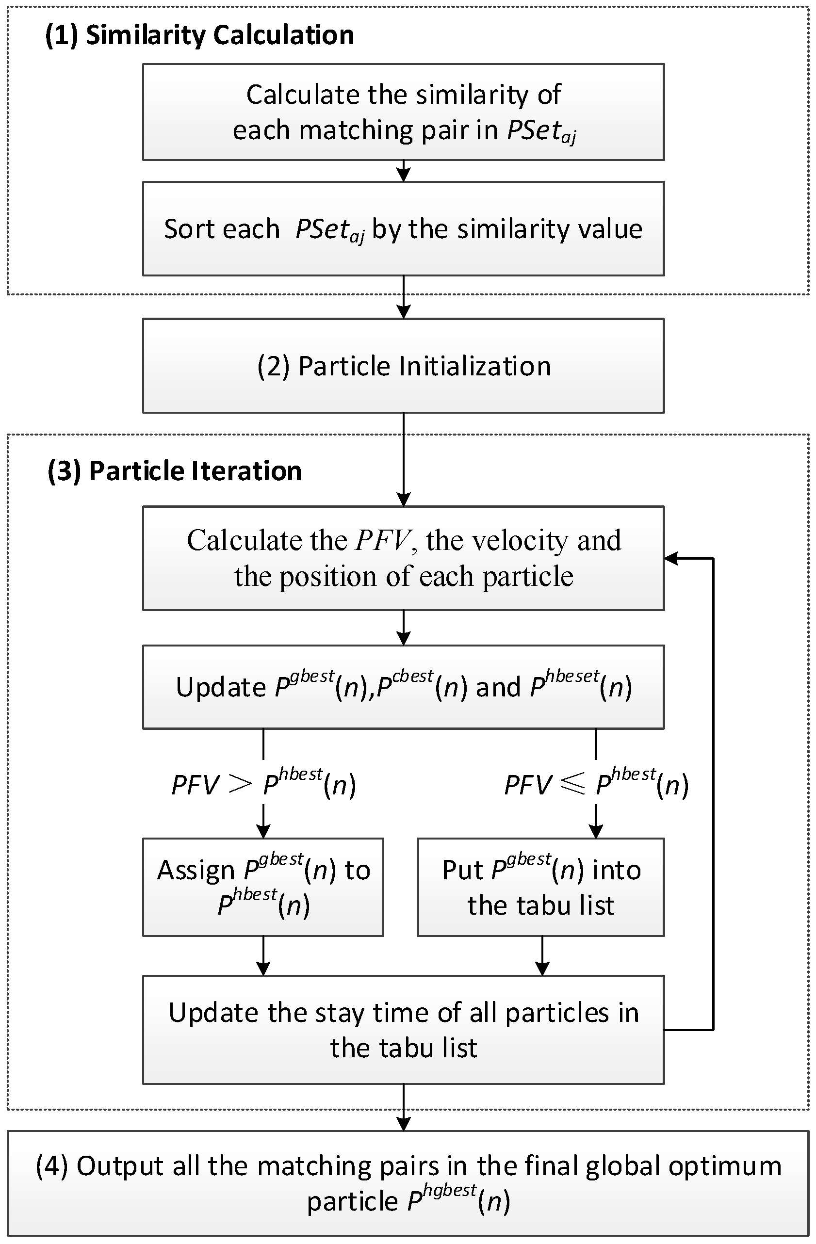
2.3. PSOM Workflow
- (1)
- Similarity calculation. For all nodes in Ra, calculate the similarity value of each matching pair in PSetaj using Equation (2), and sort PSetaj by the similarity value.
- (2)
- Particle Initialization. Initialize particles in a random manner, and select Pgbest(n), putting into the tabu list.
- (3)
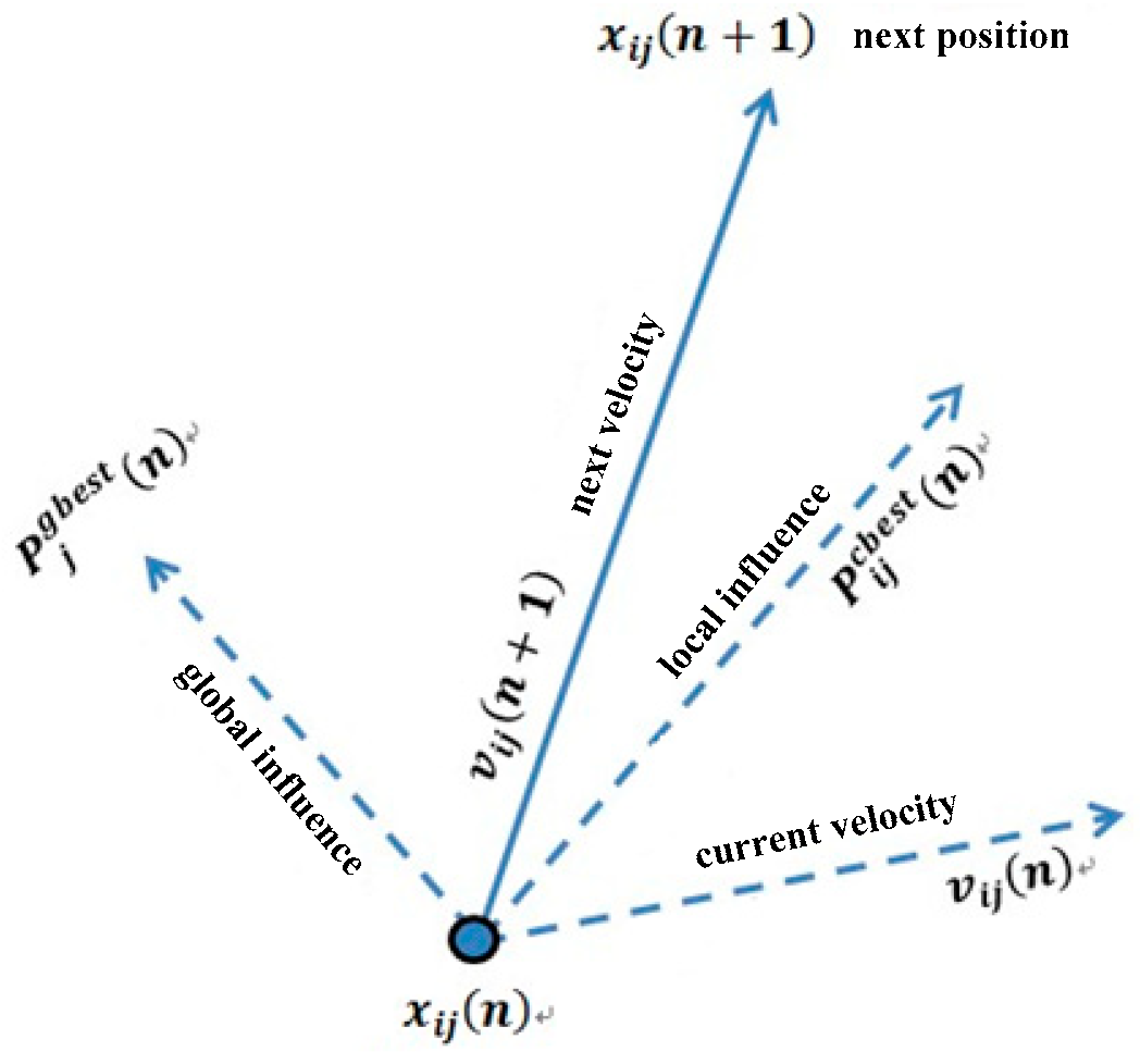
- Particle Iteration. Calculate and update the velocity and position of each particle using Equations (5) and (6). Calculate the PFV for all particles at iteration n using Equation (1), and the maximum particle is selected to be Pgbest(n). If the PFV is greater than Phgbest(n), the maximum particle is assigned to Phgbest(n); otherwise, Pgbest(n) is put into the tabu list if it is not contained. The global optimal model Pgbest(n) and the personal best model (n) are updated and recorded in each iteration. Continue with this step until the maximum iteration number is reached.
- (4)
- Output all the matching pairs in the final global optimum particle Phgbest(n).
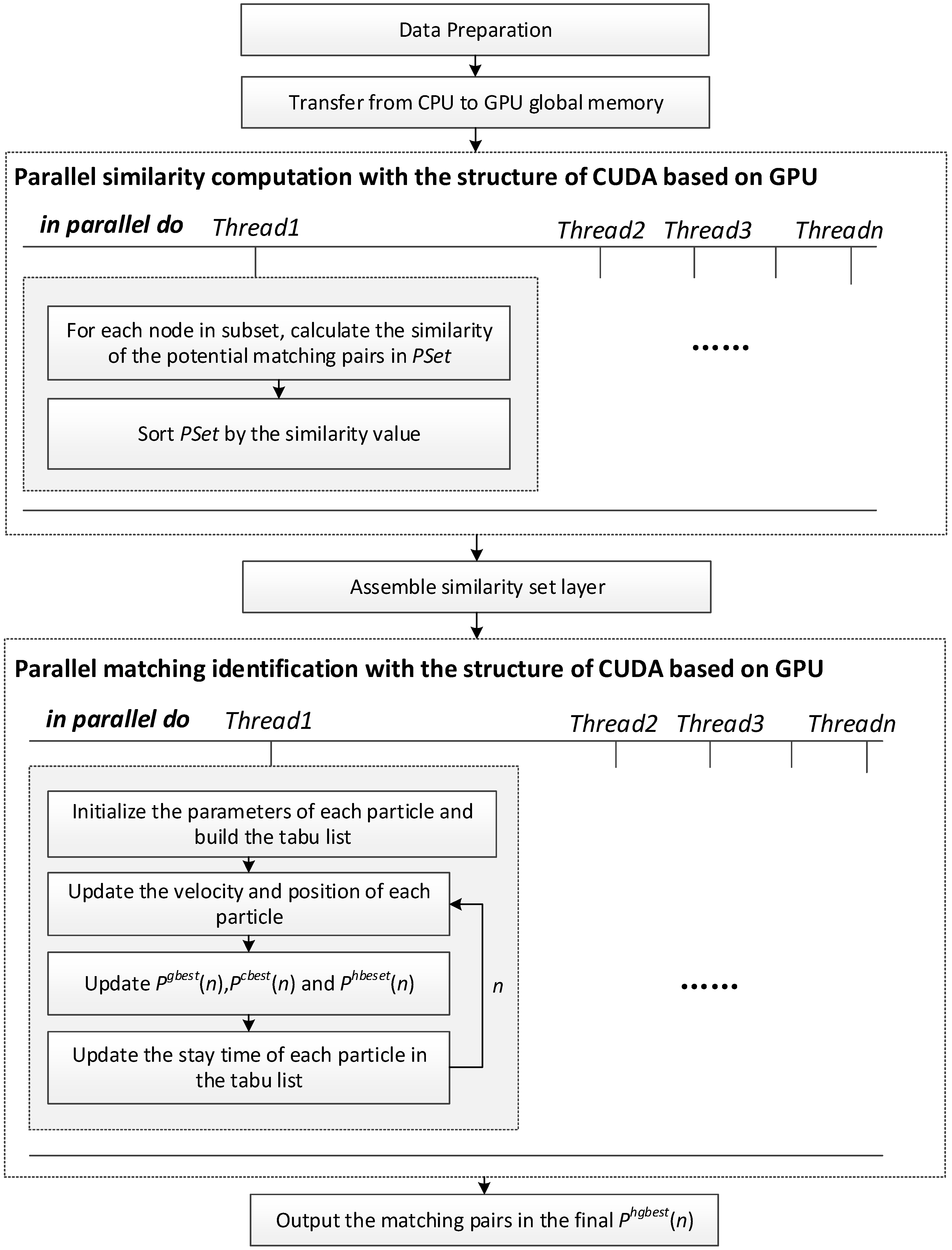
3. PSOM Parallelization Strategy
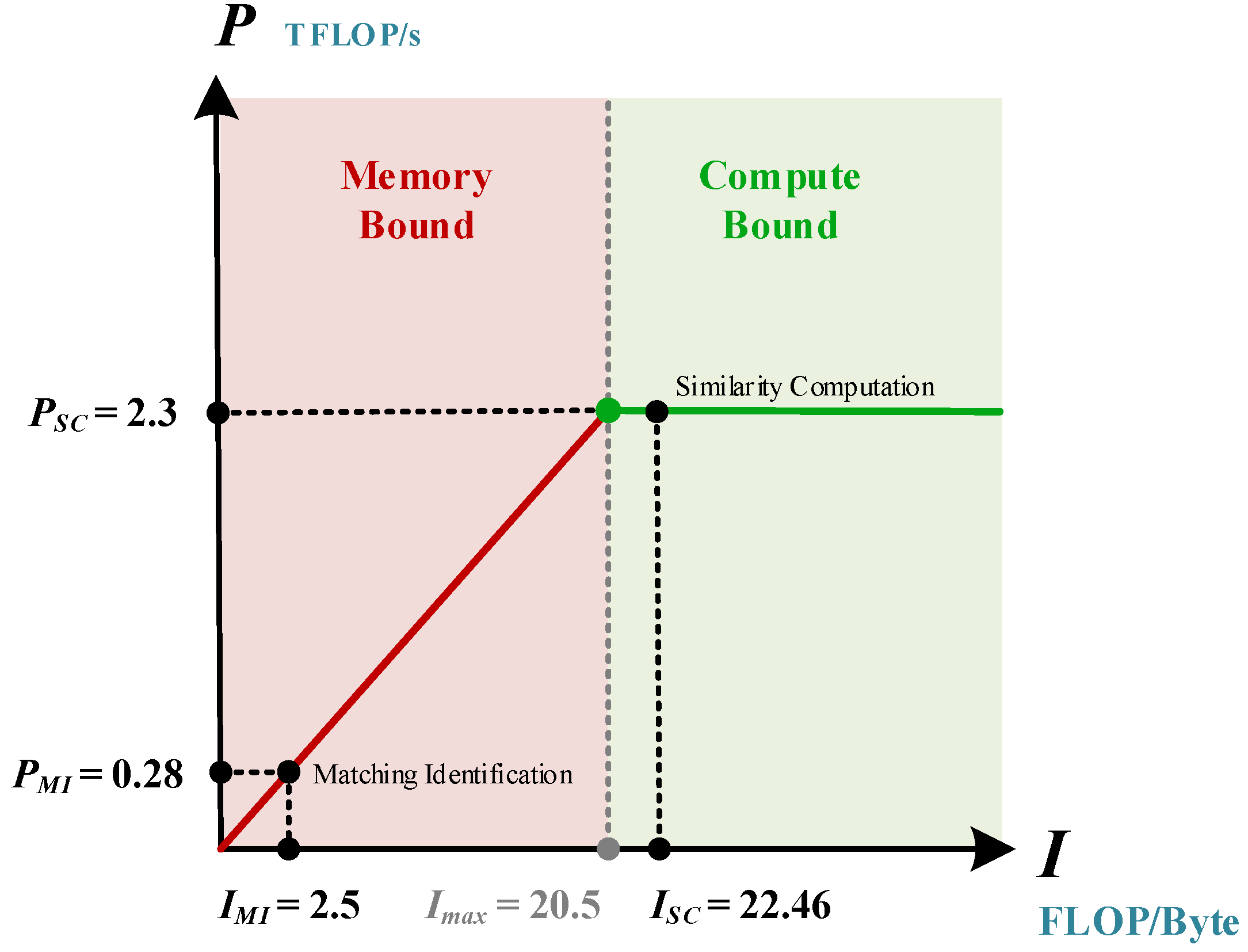
3.1. Parallel-Similarity Computation
3.2. Parallel-Matching Identification
| Algorithm 1: Parallel-Matching Relationship Identification |
| Input: |
| Road-network data in a defined GPU data structure; similarity set layer. |
| Output: |
| Matching relationship between road-network Ra and Rb. |
| Steps: |
| 1: Execute kernel function k-particle-initial. |
| 1.1: Number of threads is determined according to number of particles. |
| 1.2: The curand function is used to randomly set the initial position of each particle. |
| 1.3: Global optimal value and local optimal value are found in the first thread. |
| 2: While iteration condition not reached do |
| kernel function k-particle-fly. |
| 2.1: The velocity of each particle is calculated according to Equation (5) |
| 2.2: The position of each particle is updated according to Equation (6) |
| 2.3: The PFV of each particle is calculated. |
| 2.4: When all particles are done, the Pcbest(n) and Phbest(n) of each particle and Pgbest(n) of the whole particle swarm are updated. |
| 2.5: If PFV of the current particle is greater than Phbest(n), then the Pgbest(n) is assigned to Phbest(n). Otherwise, Pgbest(n) is put into the tabu list. |
| 2.6: The stay time of all particles in the tabu list is updated. |
| 3. If the iteration condition is reached then |
| the best particle found in the global memory is transferred from the GPU to the CPU. |
| 4. Return the matching pairs in the final global optimum particle Phgbest(n), the algorithm ends. |
4. Model Evaluation Indices
5. Results and Discussion
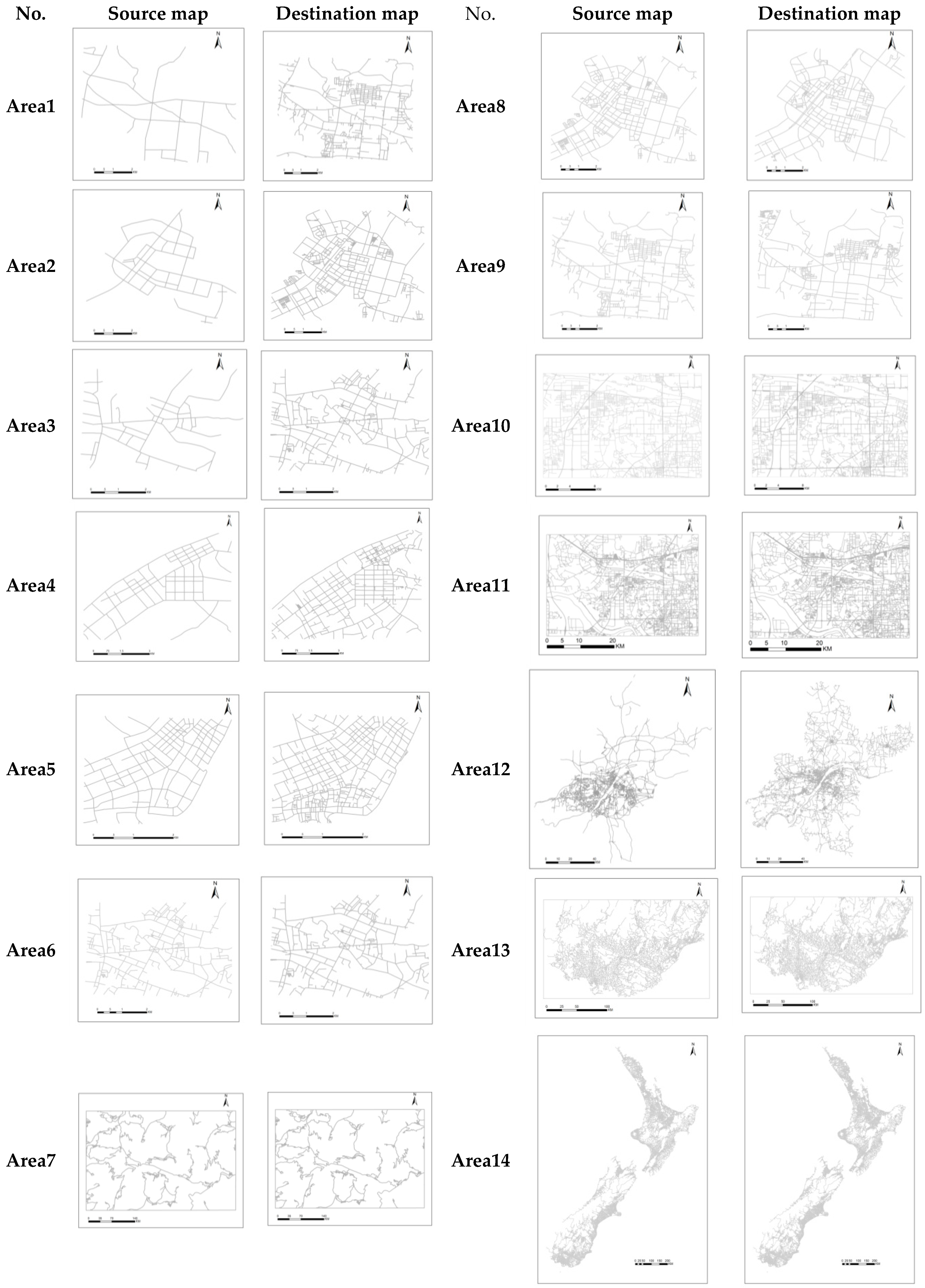
5.1. Experimental Environment and Data
5.2. Parameter Setting
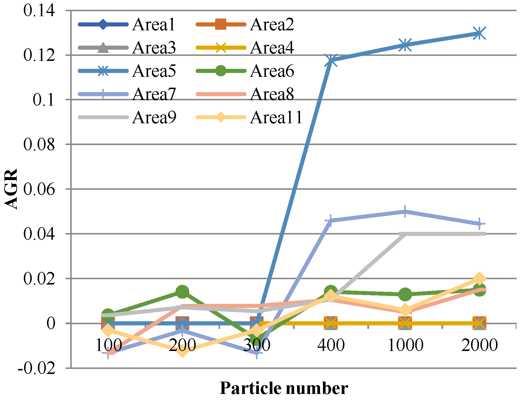
5.3. Algorithm Accuracy
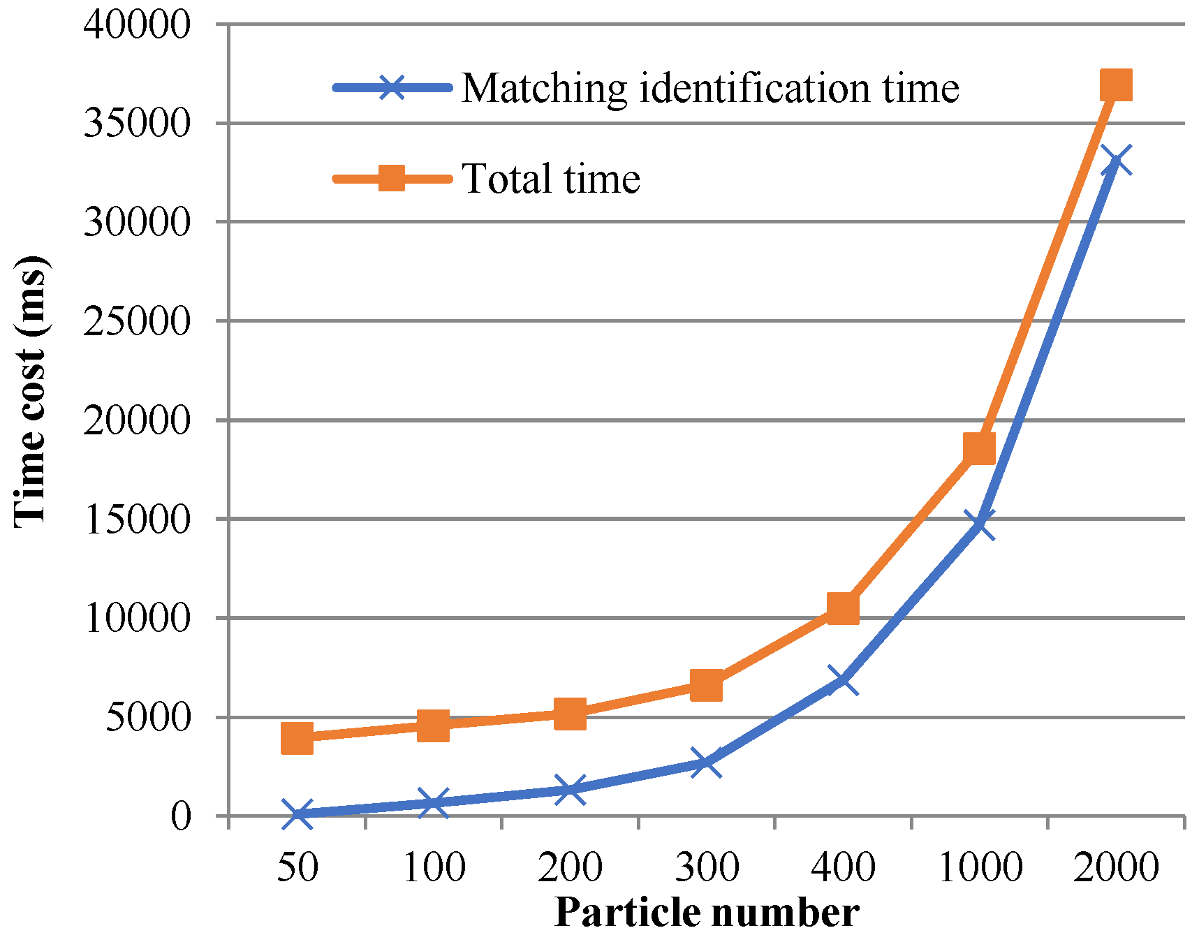
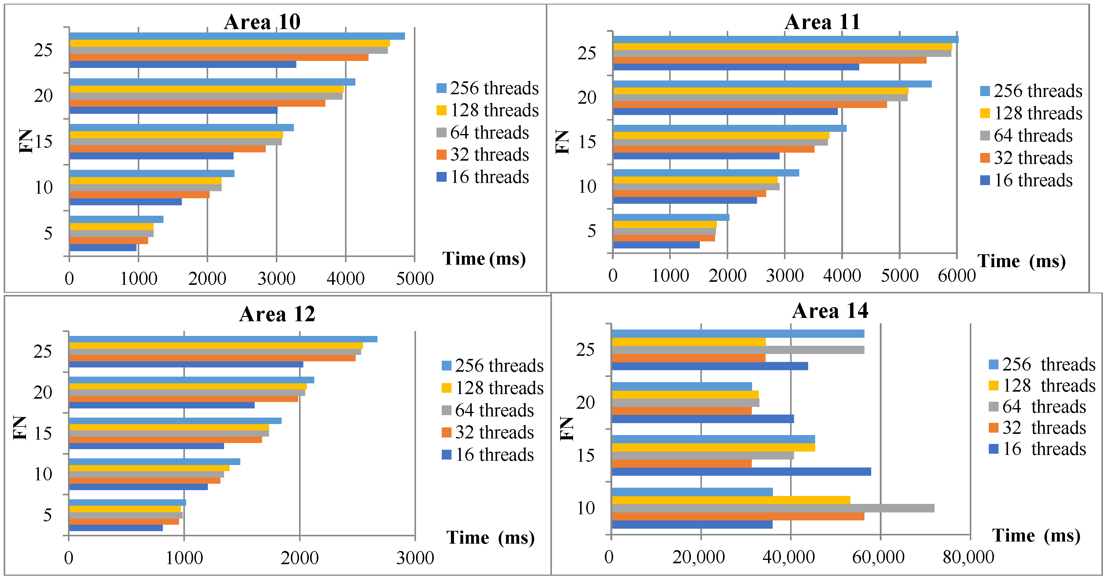
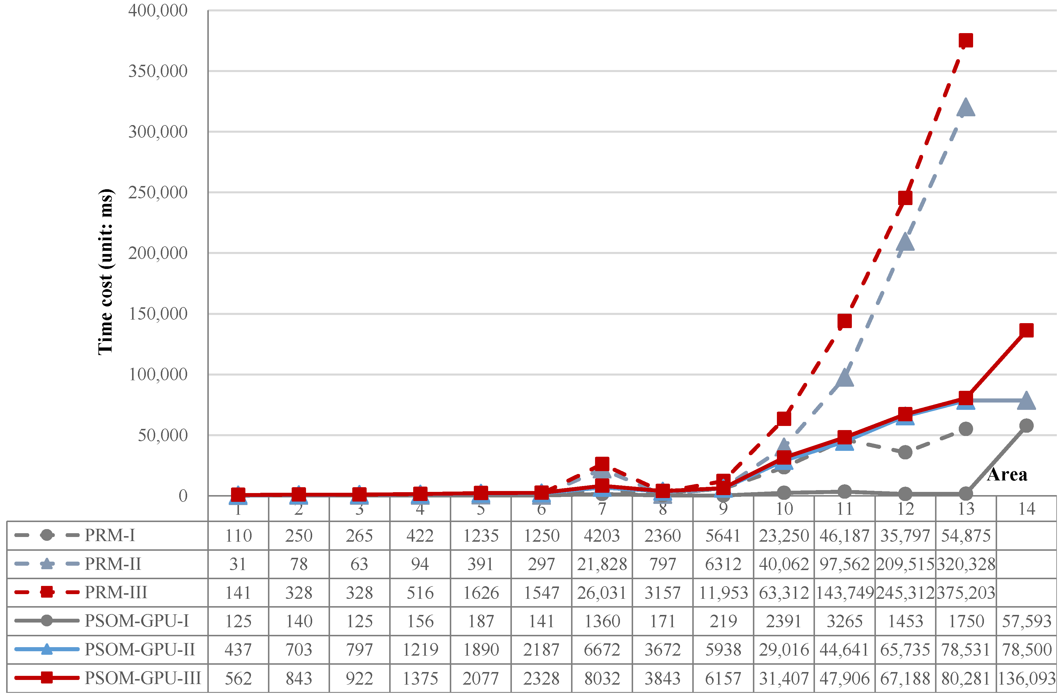
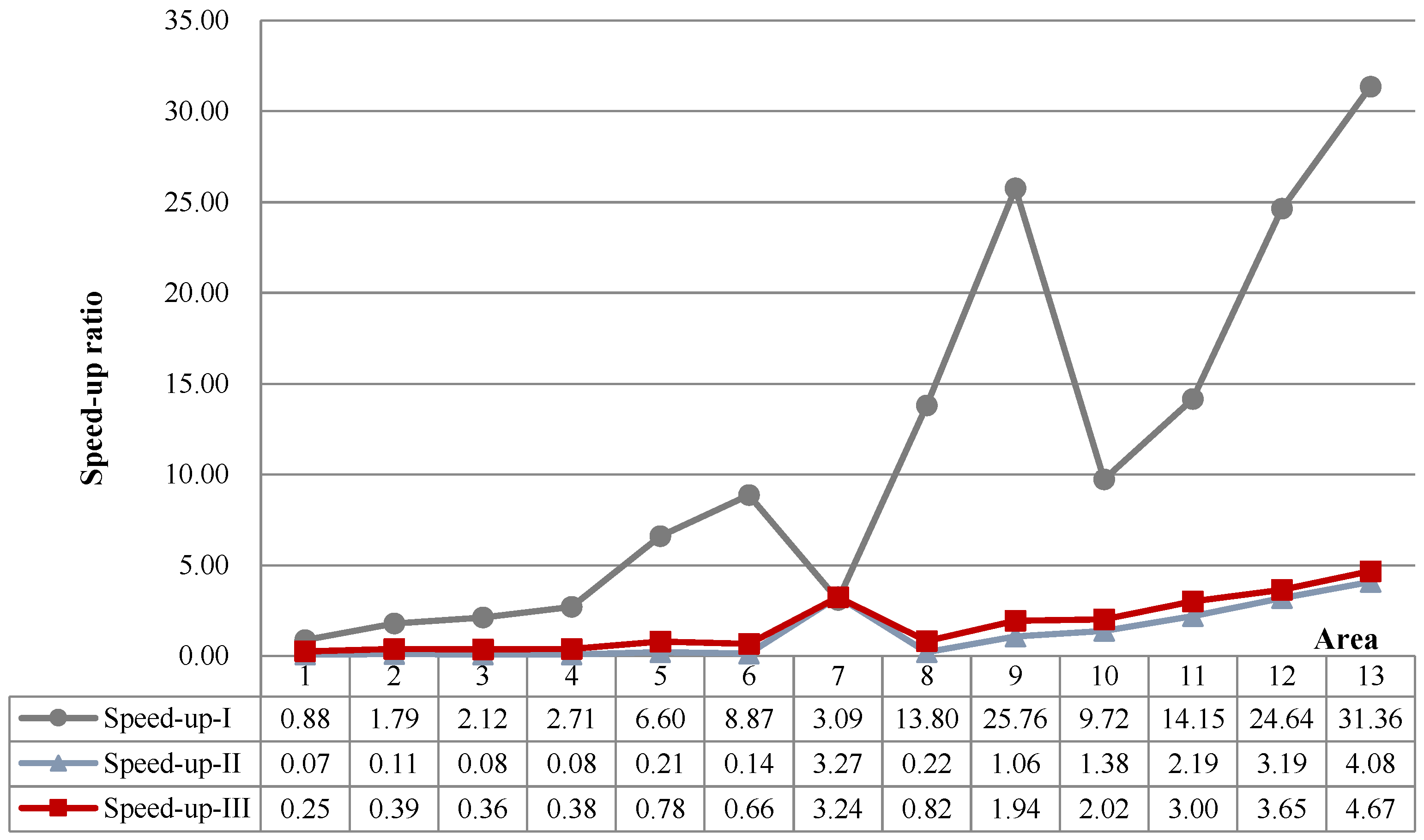
5.4. Algorithm Performance
6. Conclusions
Author Contributions
Funding
Acknowledgments
Conflicts of Interest
Appendix A
Appendix B

References
- Li, L.; Goodchild, M.F. An optimisation model for linear feature matching in geographical data conflation. Int. J. Image Data Fusion 2011, 2, 309–328. [Google Scholar] [CrossRef]
- Walter, V.; Fritsch, D. Matching spatial data sets: A statistical approach. Int. J. Geogr. Inf. Sci. 1999, 13, 445–473. [Google Scholar] [CrossRef]
- Yang, B.; Luan, X.; Zhang, Y. A pattern—Based approach for matching nodes in heterogeneous urban road networks. Trans. GIS 2014, 18, 718–739. [Google Scholar] [CrossRef]
- Beeri, C.; Kanza, Y.; Safra, E.; Sagiv, Y. Object fusion in geographic information systems. In Proceedings of the Thirtieth International Conference on Very Large Data Bases-Volume 30, Toronto, ON, Canada, 31 August–3 September 2004; Morgan Kaufmann: Toronto, ON, Canada, 2004; pp. 816–827. [Google Scholar]
- Song, W.; Keller, J.M.; Haithcoat, T.L.; Davis, C.H. Relaxation—Based point feature matching for vector map conflation. Trans. GIS 2011, 15, 43–60. [Google Scholar] [CrossRef]
- Safra, E.; Kanza, Y.; Sagiv, Y.; Doytsher, Y. Ad hoc matching of vectorial road networks. Int. J. Geogr. Inf. Sci. 2013, 27, 114–153. [Google Scholar] [CrossRef]
- Min, D.; Zhilin, L.; Xiaoyong, C. Extended hausdorff distance for spatial objects in gis. Int. J. Geogr. Inf. Sci. 2007, 21, 459–475. [Google Scholar] [CrossRef]
- Tong, X.; Liang, D.; Jin, Y. A linear road object matching method for conflation based on optimization and logistic regression. Int. J. Geogr. Inf. Sci. 2014, 28, 824–846. [Google Scholar] [CrossRef]
- Zhang, M.; Meng, L. Delimited stroke oriented algorithm-working principle and implementation for the matching of road networks. Geogr. Inf. Sci. 2008, 14, 44–53. [Google Scholar] [CrossRef]
- Xiong, D.; Sperling, J. Semiautomated matching for network database integration. ISPRS J. Photogramm. Remote Sens. 2004, 59, 35–46. [Google Scholar] [CrossRef]
- Gabay, Y.; Doytsher, Y. Automatic adjustment of line maps. In Proceedings of the GIS/LIS ‘94, Phoenix, AZ, USA, 25–27 October 1994; pp. 191–199. [Google Scholar]
- Cueto, K. A feature-based approach to conflation of geospatial sources. Int. J. Geogr. Inf. Sci. 2004, 18, 459–489. [Google Scholar]
- Yang, L.; Wan, B.; Wang, R.; Zuo, Z.; An, X. Matching road network based on the structural relationship constraint of hierarchical strokes. Geomat. Inf. Sci. Wuhan Univ. 2015, 40, 1661–1668. [Google Scholar]
- Zhao, D.; Sheng, Y. Research on automatic matching of vector road networks based on global optimization. Acta Geod. Cartogr. Sin. 2010, 39, 416–421. [Google Scholar]
- Zhang, Y.; Yang, B.; Luan, X. Automated matching crowdsourcing road networks using probabilistic relaxation. Acta Geod. Cartogr. Sin. 2012, 41, 933–939. [Google Scholar] [CrossRef]
- Luan, X. A structure-based approach for matching road junctions with different coordinate systems. In Proceedings of the Twenty-Second ISPRS Congress, Melbourne, Australia, 25 August–1 September 2012; pp. 41–46. [Google Scholar]
- Liu, C.; Qian, H.; Xiao, W.; Haiwei, H.E.; Chen, J. A linkage matching method for road networks considering the similarity of upper and lower spatial relation. Acta Geod. Cartogr. Sin. 2016, 45, 281–286. [Google Scholar]
- Fan, H.; Yang, B.; Zipf, A.; Rousell, A. A polygon-based approach for matching openstreetmap road networks with regional transit authority data. Int. J. Geogr. Inf. Sci. 2016, 30, 748–764. [Google Scholar] [CrossRef]
- Zhang, J.; Wang, Y.; Zhao, W. An improved probabilistic relaxation method for matching multi-scale road networks. Int. J. Dig. Earth 2018, 11, 1–21. [Google Scholar] [CrossRef]
- Luu, K.; Noble, M.; Gesret, A.; Belayouni, N.; Roux, P.F. A parallel competitive particle swarm optimization for non-linear first arrival traveltime tomography and uncertainty quantification. Comput. Geosci. 2018, 113, 81–93. [Google Scholar] [CrossRef]
- Yang, B.; Zhang, Y.; Luan, X. A probabilistic relaxation approach for matching road networks. Int. J. Geogr. Inf. Sci. 2013, 27, 319–338. [Google Scholar] [CrossRef]
- Tong, X.; Shi, W.; Deng, S. A probability-based multi-measure feature matching method in map conflation. Int. J. Remote Sens. 2009, 30, 5453–5472. [Google Scholar] [CrossRef]
- Finch, A.M.; Wilson, R.C.; Hancock, E.R. Matching Delaunay Triangulations by Probabilistic Relaxation; Springer: Berlin/Heidelberg, Germany, 1995; pp. 350–358. [Google Scholar]
- Hasan, S.; Bilash, A.; Shamsuddin, S.M.; Hassanien, A.E. Gpu-based capso with n-dimension particles. In Proceedings of the International Conference on Advanced Machine Learning Technologies and Applications, Cairo, Egypt, 22–24 February 2018; pp. 459–467. [Google Scholar]
- Dali, N.; Bouamama, S. Gpu-pso: Parallel particle swarm optimization approaches on graphical processing unit for constraint reasoning: Case of max-csps. Procedia Comput. Sci. 2015, 60, 1070–1080. [Google Scholar] [CrossRef]
- Dali, N.; Bouamama, S. Different parallelism levels using gpu for solving max-csps with pso. In Proceedings of the 2017 IEEE Congress on Evolutionary Computation, San Sebastian, Spain, 5–8 June 2017; pp. 2070–2077. [Google Scholar]
- Williams, S.; Waterman, A.; Patterson, D. Roofline: An insightful visual performance model for multicore architectures. Commun. ACM 2009, 52, 65–76. [Google Scholar] [CrossRef]


| Author (Year) | Data Scale | Time Cost | Accuracy Ratio | Recall Ratio | Environment | |
|---|---|---|---|---|---|---|
| Node Number | Segment Number | |||||
| Li (2010) [1] | / | 434/423 | 31 min 39 s | 98% | - | - |
| - | 308/264 | 23 min 16 s | 97.58% | |||
| - | 377/374 | 1 min 37 s | 97.85% | |||
| - | 344/322 | 2 h 6 min 14 s | 95.03% | |||
| Tong (2014) [8] | - | 99/84 | 1.8 s | 91.8% | 100% | MATLAB 6.0, Intel Core 5 Duo processor, and 4 GB memory. |
| - | 116/112 | 3.83 s | 96.1% | 96.1% | ||
| - | 137/108 | 4.71 s | 87.2% | 91.2% | ||
| Zhang (2012) [15] | 249/387 (Wuhan) | 358/577 (Wuhan) | 4 s per iteration | 97.2% | 91.2% | Microsoft Visual Studio 2008 (C# Programming Language) and ArcGIS Engine 9.3. |
| 1059/1299 (Beijing) | 1567/2019 (Beijing) | 5 s per iteration | 96.5% | 94.6% | ||
| 2732/1666 (Zurich) | 3995/2489(Zurich) | 30 s per iteration | 96.5% | 94.7% | ||
| Luan (2012) [16] | 700 | - | 13.5 min | 86.11% | 90.30% | CPU 3.06 GHz and 1 GB of RAM. |
| Yang (2014) [3] | 756/361 | - | - | 95.45% | 98.91% | - |
| Liu (2016) [17] | - | arcs: 577/585; strokes: 136/140 (Ring and radial area) | 25.44 s | 80.67% | - | - |
| - | arcs: 522/513; strokes: 113/114 (Grid area) | 10.43 s | 76.83% | |||
| - | arcs: 1092/1101; strokes: 220/230 (Hybrid area) | 43.56 s | 83.33% | |||
| Zhao (2010) [14] | 121/261 | 142/325 | 71 s | - | - | C# Programming Language and ArcGIS Engine 9.2 |
| Fan (2016) [18] | - | 12208/5945 (Heidelberg) | 22 min | 98.3% | 95.3% | - |
| - | 107438/61559 (Shanghai) | 142 min | 96.9% | 85.6% | ||
| Zhang (2018) [19] | 474/671 (Beijing) | 784/962 (Beijing) | 44 s | 95.3% | 95.0% | C #, ArcEngine10.1, CPU Intel Core 2 Duo E7200, 3.53 GHz. |
| 1556/2229 (Shanghai) | 3250/4480 (Shanghai) | 247 s | 95.1% | 95.9% | ||
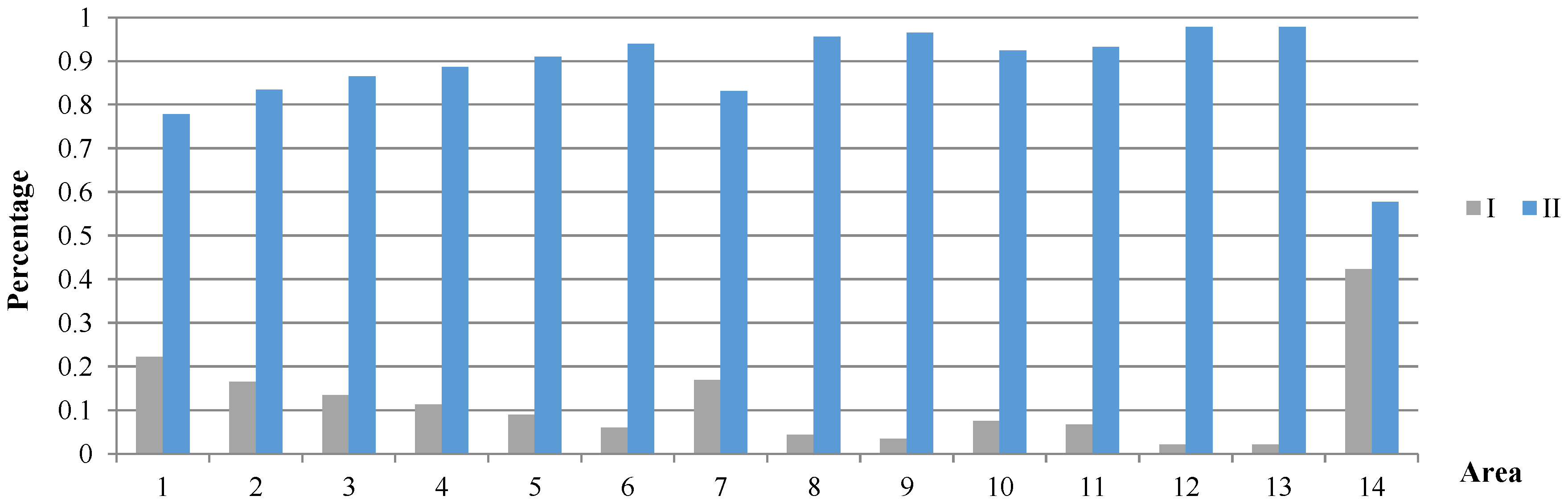
| No. | NS | ND | No. | NS | ND |
|---|---|---|---|---|---|
| Area 1 | 44 | 582 | Area 8 | 519 | 673 |
| Area 2 | 68 | 673 | Area 9 | 582 | 825 |
| Area 3 | 82 | 396 | Area 10 | 4938 | 5530 |
| Area 4 | 110 | 494 | Area 11 | 7738 | 9049 |
| Area 5 | 176 | 540 | Area 12 | 10,820 | 13,961 |
| Area 6 | 382 | 396 | Area 13 | 13,815 | 16,771 |
| Area 7 | 478 | 493 | Area 14 | 72,130 | 127,205 |
© 2018 by the authors. Licensee MDPI, Basel, Switzerland. This article is an open access article distributed under the terms and conditions of the Creative Commons Attribution (CC BY) license (http://creativecommons.org/licenses/by/4.0/).
Share and Cite
Wan, B.; Yang, L.; Zhou, S.; Wang, R.; Wang, D.; Zhen, W. A Parallel-Computing Approach for Vector Road-Network Matching Using GPU Architecture. ISPRS Int. J. Geo-Inf. 2018, 7, 472. https://0-doi-org.brum.beds.ac.uk/10.3390/ijgi7120472
Wan B, Yang L, Zhou S, Wang R, Wang D, Zhen W. A Parallel-Computing Approach for Vector Road-Network Matching Using GPU Architecture. ISPRS International Journal of Geo-Information. 2018; 7(12):472. https://0-doi-org.brum.beds.ac.uk/10.3390/ijgi7120472
Chicago/Turabian StyleWan, Bo, Lin Yang, Shunping Zhou, Run Wang, Dezhi Wang, and Wenjie Zhen. 2018. "A Parallel-Computing Approach for Vector Road-Network Matching Using GPU Architecture" ISPRS International Journal of Geo-Information 7, no. 12: 472. https://0-doi-org.brum.beds.ac.uk/10.3390/ijgi7120472