Assessment of Displacements of Linestrings Based on Homologous Vertexes


Department of Cartographic, Geodetic Engineering and Photogrammetry, University of Jaén, Campus Las Lagunillas, Edificio A3, 23071 Jaén, Spain
*
Author to whom correspondence should be addressed.
ISPRS Int. J. Geo-Inf. 2018, 7(12), 473; https://0-doi-org.brum.beds.ac.uk/10.3390/ijgi7120473
Submission received: 6 November 2018
/
Revised: 29 November 2018
/
Accepted: 6 December 2018
/
Published: 9 December 2018
Abstract
:This study describes a new method that was developed in order to assess the displacements between two linestrings that represent the same element in two datasets based on their shape. Until now, all existing line-based methods have been focused on the calculation of distances or buffer inclusions between the two linestrings. However, these approaches assess a spatial difference between two linestrings, but they can hide the displacements that were suffered because of the geometry of the linestrings themselves. In our approach, the shapes of the linestrings are taken into account in order to identify homologous vertexes and estimate real displacements. Between two lines a pair of homologous vertices are defined as those that represent in reality the same characteristic feature of the line. Homologous vertexes can be detected by means of any appropriate algorithm. In order to test this method, we developed a design of experiment that was based on its application to a large dataset of lines classified into five sinuosity classes. These datasets were obtained from an external source that contains perturbed linestrings with several known random and systematic disturbances. 496 linestrings and 59 configurations were used in this experiment. The results have demonstrated the viability of the proposed method in estimating the real displacement of the lines, and consequently assessing their positional accuracy.
1. Introduction
One of the most important types of data of the vector geographical databases is linestrings. Linestrings (also called lines in this paper) are used to represent those real phenomena that present a linear spatial behavior, while taking into account the scale of the data. For example, lines are usually used to represent rivers, roads, railways, etc. In addition the use of mobile devices is also generating a great amount of georeferenced data, which are usually considered as lines, such as the Global Navigation Satellite System (GNSS) tracks of routes. These lines can also be shared on the Internet as Volunteered Geographical Information (VGI) [1] while using several applications (e.g., Wikiloc: https://www.wikiloc.com) or they can even be used for the generation of cooperative maps (e.g., OpenStreetMap: https://www.openstreetmap.org). We can definitely highlight the extensive use of lines for representing the linear features of GI, including that of non-expert users, and the increasing interest both of producers and users in the quality, and more specifically in the positional accuracy of data and specifically of linestring data. In this case, positional accuracy means displacement between two linestrings, an instance (assessed line) and a reference (assessor line). One of the main characteristics of lines is their shape. Consequently, we can take advantage of this aspect to analyze the displacements between two lines. Shape describes the geometric form of individual spatial objects [2]. In this context, shape analysis is the process of building fundamental units for identifying and describing patterns [3]. One of the main algorithms that was developed until now to analyze the shape of geometries is the Turning Function described by Arkin et al. [4]. Initially developed to analyze polygons, it considers the angle of the counter clockwise tangent as a function of the arc length. The length of the polygon’s perimeter line is scaled from 0 to 1. The comparison between two polygons is derived from a distance function between the turning functions of both elements.
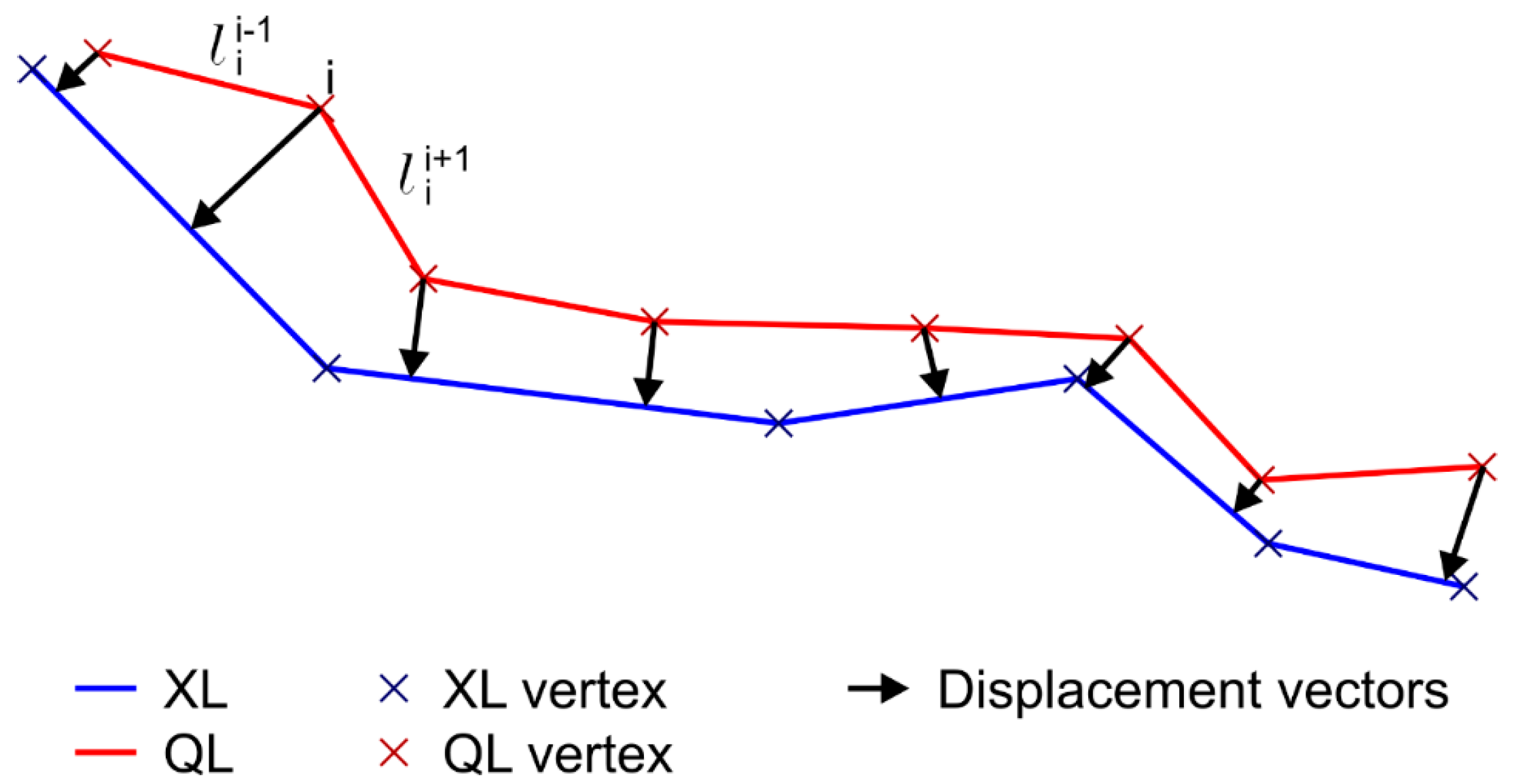
The positional accuracy of lines is estimated using methods and metrics that were developed by several authors based on the concept of distance between lines. The Epsilon Band model [5] establishes a band around the most probable position of the line. This band was initially described through two parallel lines tangent to the standard error circles at the extremes of the line. Since then, some extended models of bands have been described [6,7,8]. Alternatively, Shi and Liu [9] propose a band that is based on the stochastic process theory, and Heuvelink et al. [10] and Wu and Liu [11] described bands that are based on probability distribution functions. A complete review of these models of uncertainty referring both to segments and lines was described by Gil-de la Vega et al. [12]. Based on these and other models, some methods and metrics have been described in order to assess differences between two lines. In general, they can be divided into three types: (i) firstly, those based on the comparison of characteristic parameters (scalar values) obtained in both lines, e.g., metrics such as length, density, angularity, and curvilinearity, which were proposed by McMaster [13] for comparing original and simplified lines and extended by Jasinski [14] and Lawford [15]; (ii) secondly, those methods that are based on the calculation of distance and area between both lines, e.g., Areal Index and the Vector Displacement [13], the Hausdorff Distance Method (HDM) extended by Abbas et al. [16], the Average Distance Method (ADM), the Epsilon Band Method (EBM) extended by Mozas-Calvache and Ariza-López [17], and the Vertex Influence Method (VIM) [18]. Some of these methods were extended to three-dimensional (3D) assessments by Mozas-Calvache and Ariza-López [19]; (iii) thirdly, the methods based on buffers generation, such as the Single Buffer Overlay Method (SBOM) [20] and the Double Buffer Overlay Method (DBOM) [21], where the percentage of inclusion (SBOM) or the mean displacement (DBOM) are derived from several buffers’ widths. Some studies [12,19] undertook a broader analysis of these methods. All of these methods presented advantages and disadvantages. We consider that the methods of classes 2 and 3 are the most suitable, since class 1 does not take into account the position of the elements. On the other hand class 3 methods, which are based on buffers, are more complex to program and they are also problematic when the lines are long and complex. Therefore, we prefer distance-based methods (class 2). However, we highlight the one that was used in this study, which is the VIM [18]. This method is easy to implement and it has the possibility of assessment of lines in 3D [19]. When considering one line to be assessed (XL) and using as reference element (QL), the same line that was obtained from another source (a more accurate source for a quality control), the VIM method consists of the determination of the displacement vectors from all the vertexes of QL to the closest points of XL (vertex or interpolated points on segments), and the obtaining of a mean displacement vector, and consequently a mean value of displacement, by weighting all of the vectors that were obtained by the length of the adjacent segments to each implicated vertex i (Figure 1). Obviously, we must consider homologous lines (XL and QL) to apply this assessment. Therefore, a previous stage to determine pairs of homologous lines must be developed using matching techniques. The matching of homologous elements (roads and road’s networks, rivers and river’s networks, buildings, etc.), is a key matter in geosciences, because the conflation of different datasets is an actual need with different aims, for instance, Asakura et al. [22] propose a matching algorithm for sharing information among refugees in disaster areas. Xi et al. [23] offer a general view of map matching algorithms and its application. The matching of road’s networks has been treated by numerous authors, Quddus et al. [24] offer an overview of algorithms and numerous references. Matching of river’s networks has a different treatment from that of roads because of the difference in the nature of the network itself. Kieler et al. [25] offer an interesting approach to this problem in order to conflate datasets of different scales. Reinoso [26] has analyzed the matching of elevation contours with an interesting analytical approach that can be extended to other cases (e.g., buildings footprints). Xavier et al. [27] described a detailed overview of matching techniques to determine homologous lines. In this study, we consider that matching was performed previously.
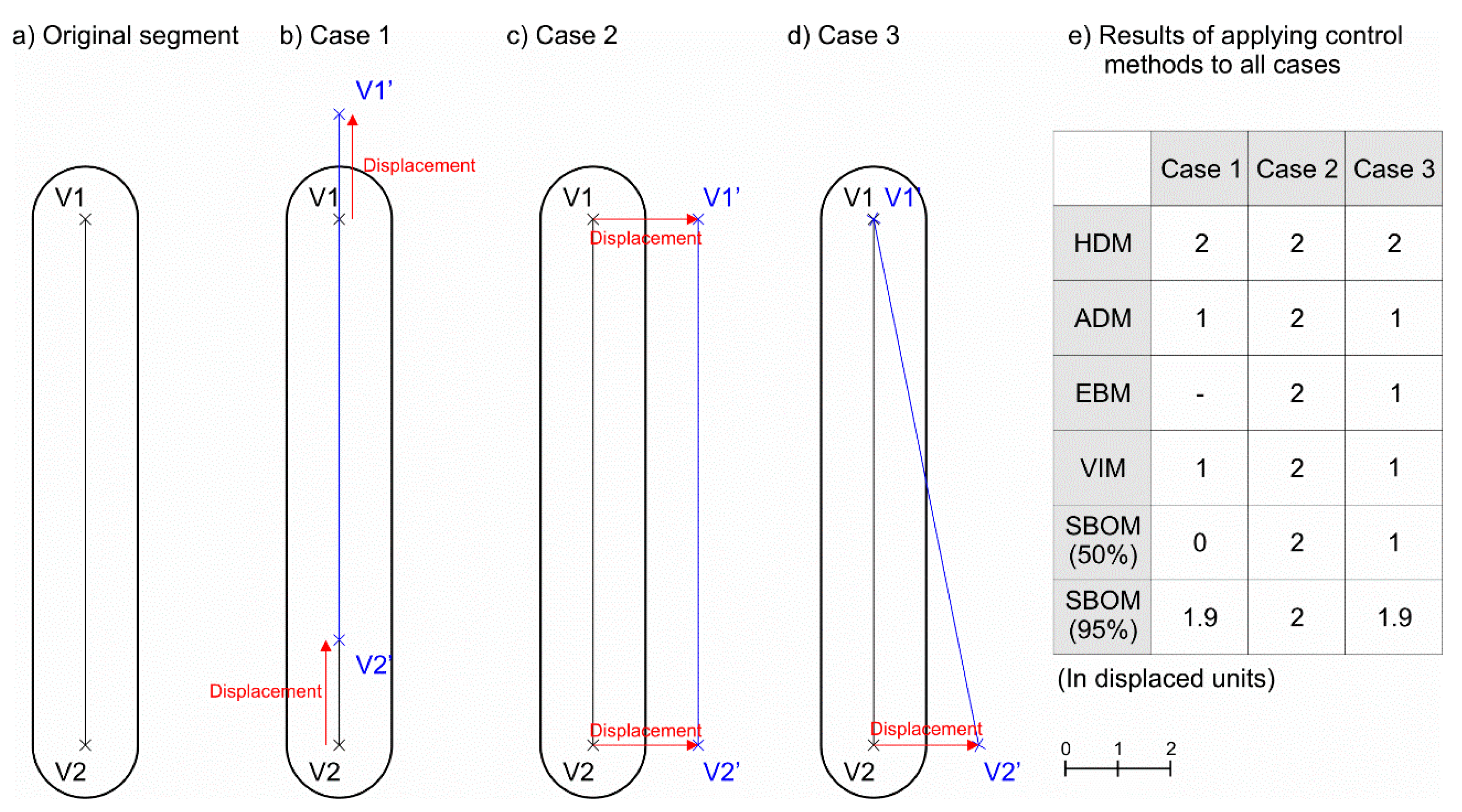
For methods of second and third classes described above, when a displacement is applied to a line it can be partially hidden by the line itself, minimizing the value of the estimated displacement. A simplified example of this issue is shown in Figure 2, which displays a segment (V1-V2) with a length of 10 units that presents a one-sigma uncertainty of one unit (Figure 2a). If a supposed displacement of two units (simulating a bias error) is applied to the segment, we obtain two extreme cases V1’-V2’ (Figure 2b,c), depending on the direction of the displacement. Case 1 (Figure 2b) shows that the segment is displaced in the same direction as the original segment, while in Case 2 (Figure 2c), the displacement is applied perpendicular to the direction of the original segment. Case 1 (Figure 2b) shows that 80% of the segment is coincident to the original segment, but this does not occur in Case 2 (Figure 2c), despite the fact that the displacement applied is the same. The results of inclusion in the uncertainty band of the displaced segment V1’-V2’ for both cases are completely different. In Case 1, 90% of the segment is inside the uncertainty band of V1-V2, while in Case 2, all the length of the segment is outside this uncertainty band. However, the value of displacement applied has been equal in both cases. The distance-based methods (ADM, EBM, and VIM) previously described detecting the displacement in Case 2 but not in Case 1 (results shown in Figure 2e), except in the case of the HDM, which detects the maximum displacement (two units in this case). In addition, the SBOM shows that 50% and 95% of inclusion in the buffers are achieved using 0 and 1.9 units in Case 1 and 2 units in Case 2. Therefore, the values using 95% are quite similar to the displacement that was applied in both cases. Another case is shown in Figure 2d, where the displacement of two units is only applied to one vertex (V2’). In this case, all methods detect the mean displacement of 1 unit except the HDM, which is very sensitive to maximum displacements (detects two units), and the SBOM (≈95%), which also overestimates the applied displacement (1.9 units), while the SBOM (≈50%) achieves the mean value of the displacement applied (one unit). Definitely, the results that were obtained using this simplified example demonstrate that these methods do not always estimate real displacements applied to the segment and in consequence to lines. This does not mean that these methods are not valid. These methods are efficient in a general situation for displacement assessment between lines, but they can minimize the results of real displacements between two lines (a maximum reduction occurs when both directions of the segment and the applied displacement coincide). They are not completely useful for estimating real displacements, as explained by Mozas-Calvache and Ariza-López [28], when they tried to detect systematic errors simulated to a set of lines.
When considering the issue previously described, the main goal of this study is the development of a new method for estimating real displacements that are suffered by lines. Our hypothesis is that the actual displacement between two lines can be measured using the displacement between homologous vertexes determined in both lines (to be assessed (XL) and to assess (QL)). We consider as homologous vertexes those that represent the same point in both lines and for which it is possible to establish a one-to-one relation. For example, both pairs of endpoints of a pair of lines are considered homologous vertexes. In this sense, we propose an adaptation of the VIM method where the displacement vectors that were obtained are not determined to the closest point of the XL line, but are referred to a homologous vertex previously determined on the XL line.
2. Materials and Methods
In this study, we develop a new method for assessing the displacements of lines in order to avoid the issues previously described. The method is based on the VIM method [18] and it is called the Vertex Influence Method by Vertexes (VIM-V). Testing the proposed VIM-V method requires a design of experiment where several known displacements are applied to a large set of lines in order to contrast its efficiency in multiple cases. More specifically, this approach has been checked using a large number of lines perturbed with random and systematic displacements (translations, rotations and scale transformations) obtained from an external source. This external source is the material used. The content of this data source means a statistical design of experiment. In this section, we first describe the material and then the method.
2.1. Material
As data input we have used a set of lines that was obtained from an external independent source. This source dataset is called MatchingLand [29]. The MatchingLand dataset is a testbed composed of geographic features (points, lines and areas) whose content is intended as an experimental design, as will be seen below.
An experimental design is the result of a design of experiments (DoE), which is a statistical technique by which it is possible to make intentional changes in some controlled factors of a system or process, notice the resulting variations in the observed variables, and then analyze the influence of those factors in these variables [30]. The main concepts around experimental design are: (1) controlled variable; (2) factor; (3) level; (4) treatment; and, (5) experimental unit. The controlled variables (dependent variables), sometimes characteristic functions, are the objective of the experiment that we want to analyze, in our case the displacement estimation. A factor is the independent variable (e.g., morphology, positional error, road category, etc.) for which we want to determine its effect over the controlled variable, and the different values of this factor are named levels (e.g., for the morphology, the five classes presented in Xavier et al. [29]. Treatment is the combination of different levels of factors considered in an experiment (e.g., the combination of morphological classes and different positional error cases). An experimental unit is the matter to which the treatments are applied. In our case, the experimental units are the instances of MatchingLand.
Major features of this source are:
- Lines are prepared with the aim of helping the evaluation of geospatial matching methods for vector data and consequently can be used to assess displacements.
- The dataset was built up from mapping data at scale 1:25,000 produced by official mapping agencies.
- The dataset offers five different morphology classes of linestrings, from very smooth to very sinuous lines (CL1 to CL5) (see [31] for details). Accordingly, we actually consider five categories of lines (each one corresponding to a sub-dataset).
- The lines of these five categories (sub-datasets) were modified applying systematic perturbations (translations, rotations, and scaling), random perturbations, and combinations of these types.
- The values of these perturbations were known, so we were able to use them to see if our method can properly estimate them.
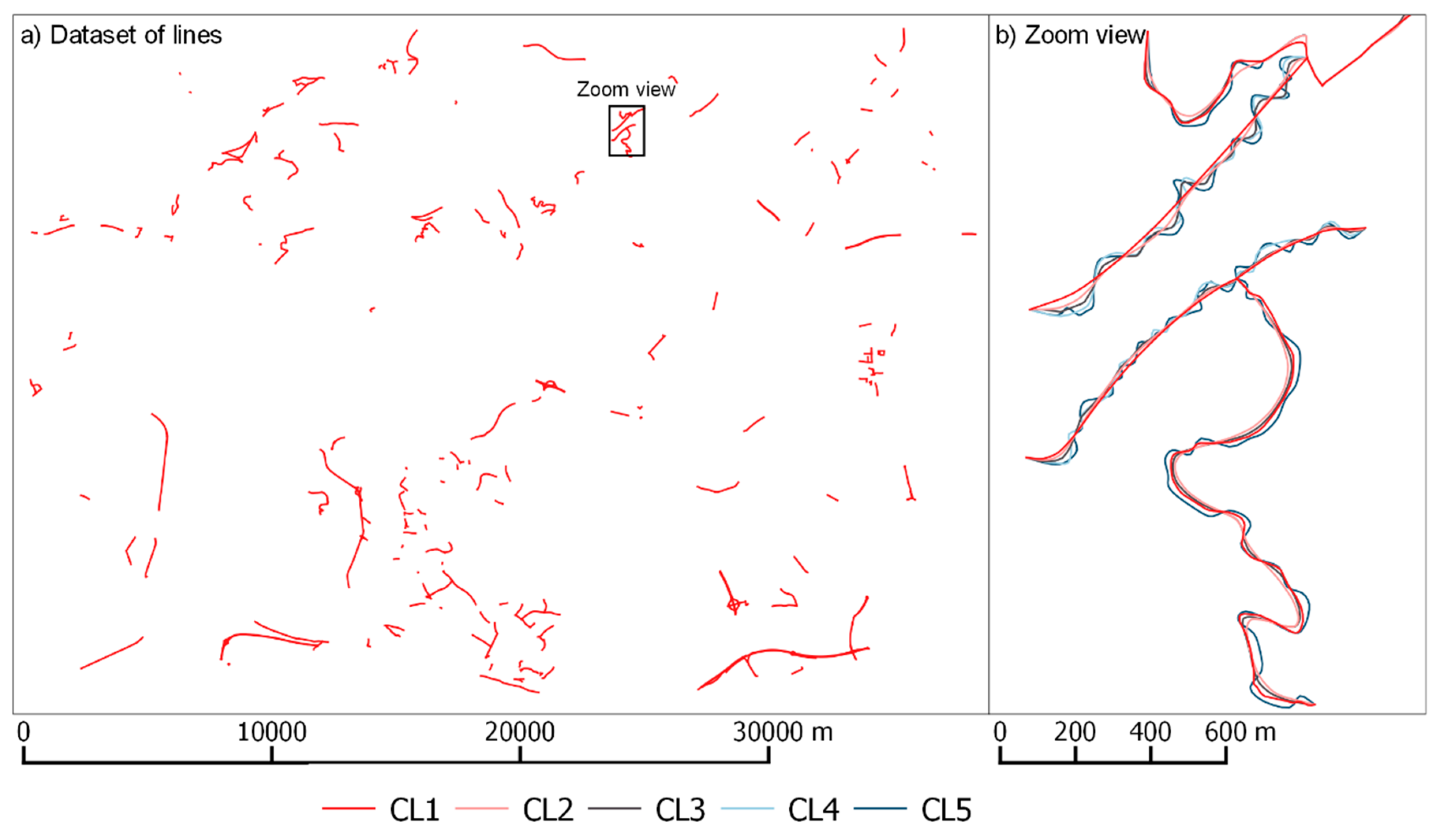
The datasets of lines that were used in this application were composed of 496 road lines (Figure 3) in each morphology category or class (CL1 to CL5). The main characteristics of these categories are shown in Table 1.
The original sets of lines were used as assessor lines (QL) in this study. As lines to be assessed (XL), several sets of perturbed lines derived from QL were obtained from MatchingLand. In this sense, the original datasets were affected by random and systematic perturbations (translations, rotations, and scaling). Some combined cases were also included. In summary we were able to use 3 sets of lines affected by random perturbations for each class CL1–CL5. This supposed 15 random cases (3 × 5). In the case of systematic perturbations, we will use 26 cases of translations, rotations, and scaling (applied both individually and combined) for each class CL1 to CL5. This allows for 130 assessments (26 × 5). Finally, 30 combined cases, including systematic and random perturbations, will be used for all morphology classes (adding 150 assessments –(30 × 5)). In total, 295 assessments can be developed between the original (QL) and the perturbed (XL) sets of lines. As mentioned previously, these 295 assessments can be applied to 496 lines.
Table 2 summarizes the 29 cases to use in this application, which can be obtained from MatchingLand, and Table 3 the 30 combined cases between random and systematic perturbations generated for this study by mixing previous cases. The three cases of random perturbations (5, 12.5, and 25 m) are coded in Table 2 and Table 3 as ra1, ra2, and ra3, respectively. MatchingLand obtained these perturbed cases using a new method of vector fields that was based on three parameters (standard displacement, field resolution, and sigma) [29]. The translation values were 5 and 12.5 m (coded as t2 and t10 in Table 2 and Table 3), which corresponded to a translation of 3.53553 m and 8.83883 m, both in X and Y. The rotations applied were 0.000521513 rad around the lower left and the center pivots (coded as r1 and r2, respectively). Finally, the scaling factors applied were 1.00052 and 0.999478 (coded as s1 and s2, respectively). Non-perturbed random, translation, rotations, and scaling cases are coded as ra0, t0, r0, and s0, respectively, in Table 2 and Table 3. More information about the obtaining of the perturbed lines is available in [29].
2.2. Method
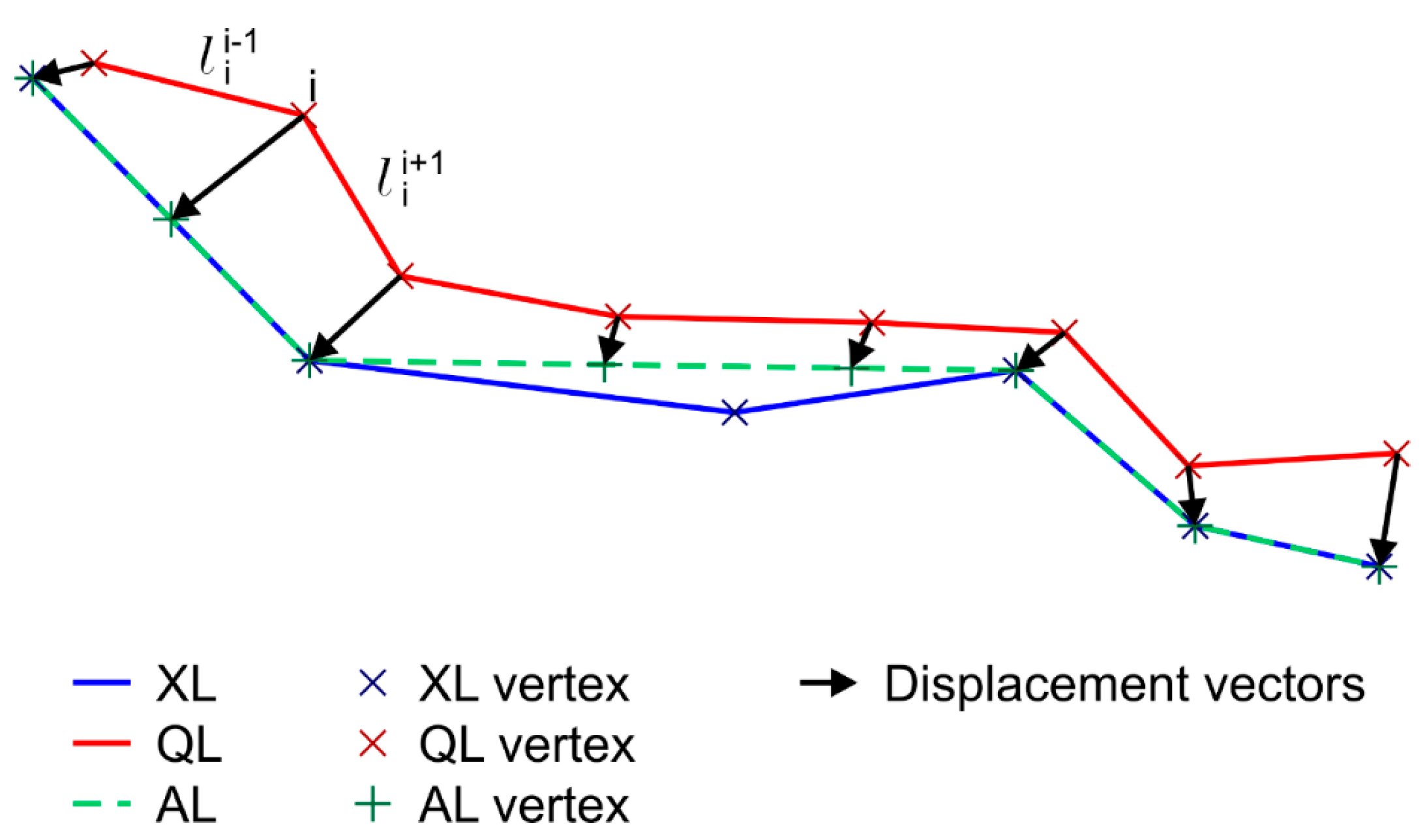
The main goal of the VIM-V method is the adaptation of the VIM method in order to estimate the real displacements that were suffered by the vertexes of the line. In this approach, the displacement vectors of VIM are not obtained between the vertexes of the QL to the closest points of the XL. Instead, they are calculated from the vertexes of the QL line to those homologous vertexes detected or defined in the XL. Unfortunately, the lines to be assessed (XL) are not usually composed of the same vertexes that define the line to be used as assessor (homologous vertexes related 1 to 1). Thus, for a general case, this approach proposes that the displacement vectors may be obtained between the vertexes of the QL and the homologous vertexes of an auxiliary line AL, which may be determined from XL when taking into account the distribution of vertexes of QL and the shape of both lines (Figure 4). As in the case of VIM, the displacement vector that was obtained in each vertex i is weighted by the length of the adjacent segments in order to provide a mean displacement vector of the line (and consequently a mean displacement value). So, the VIM-V requires that both lines be defined by the same number of vertexes and each vertex of QL must be related to another homologous vertex in XL (or AL).
Although the implementation of VIM-V is easier than VIM because the displacement vectors are directly derived from the coordinates of the vertexes once the homologous vertexes are determined, the main difficulty of this approach is related to this determination of the homologous vertexes in XL. In this method, the process of determination of the positions of the homologous vertexes is based on the shape of both lines (QL and XL). To summarize, the process is based on the generation of an auxiliary line (AL), which is defined to be as coincident as possible to XL, while taking into account that each vertex of AL must be homologous to one vertex of QL. Furthermore, this correspondence must be unique.
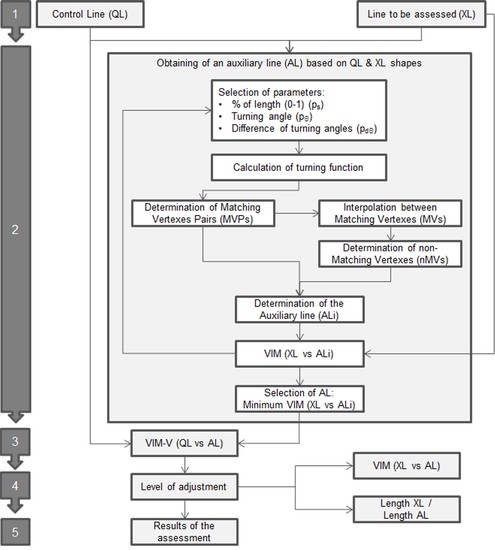
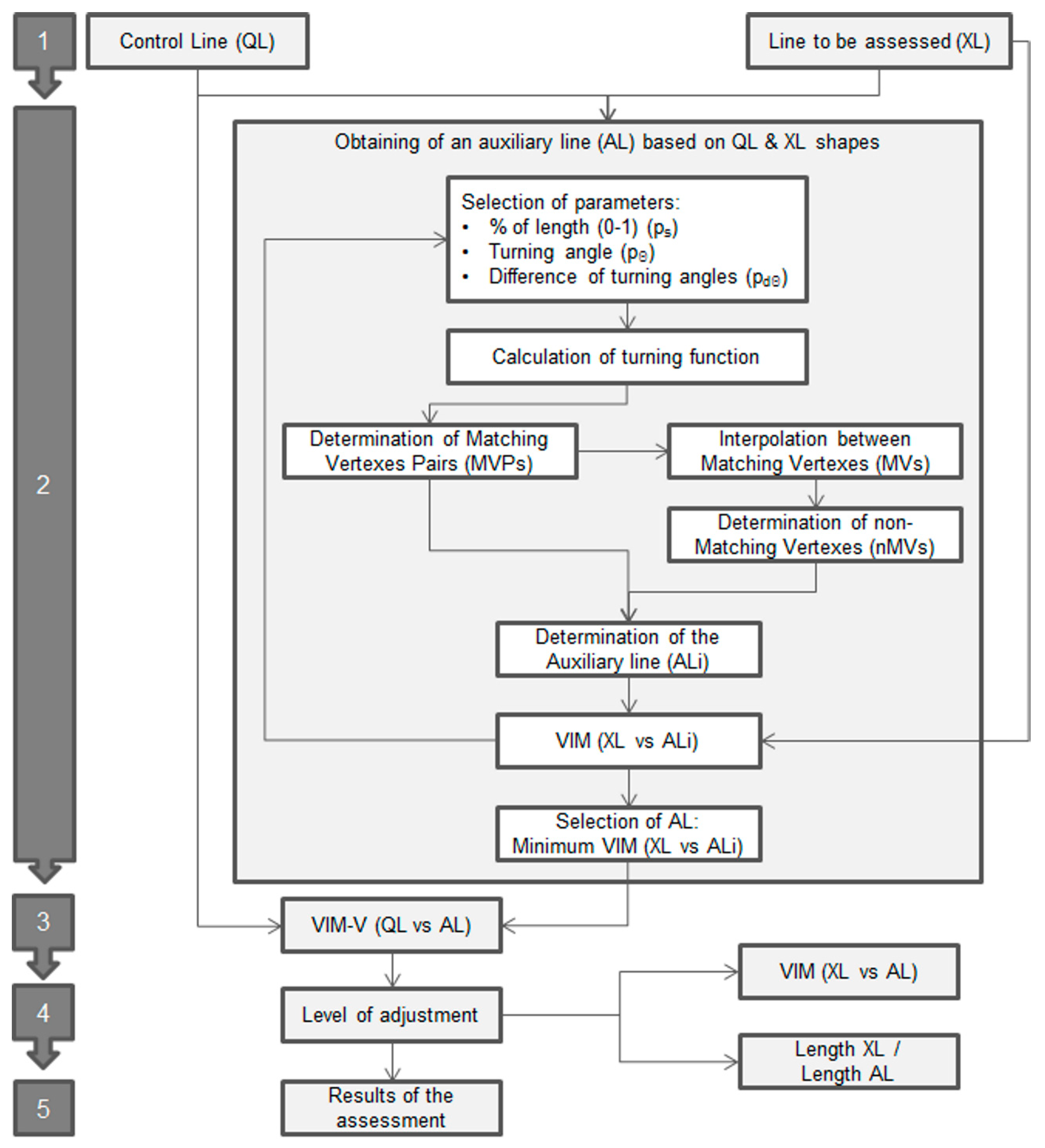
Taking into account these premises, the method proposed in this study follows the process shown in Figure 5.
- 1.
- First, the process starts with two lines: the line to be assessed (XL) and the line to assess (QL), which are obtained from a more accurate source.
- 2.
- Obtaining of an auxiliary line (AL) based on QL & XL shapes: In this stage we develop an iterative optimization procedure in order to obtain an auxiliary line (AL) which has the best adjustment to the shape of XL and is defined by the same number of vertexes of QL (following its geometrical behavior). To obtain this, we develop a procedure that is based on the comparison of the turning functions [4] of XL and QL in order to determine a set of Matching Vertexes Pairs (MVPs) that are considered as homologous in both lines (Figure 5). The turning function is adapted to linestrings considering a part of the function between two well-defined points of each line (start and end points). The turning function is obtained by scaling the length (s) of the line in the range 0 to 1 and determining the turning angles (Θ) of the segment at each vertex. This aspect is very interesting when comparing turning functions in avoiding the scale discrepancies between both lines. Obviously, the lines usually included in spatial databases present different behaviors and singularities, so we establish three parameters in order to control the process and to determine the set of MVPs between QL and XL. These parameters are:
- ps = neighborhood threshold. A maximum normalized distance [0, 1] allowable between homologous vertices of both lines. This parameter ensures that both homologous vertices are close together.
- pΘ = angle threshold. The minimum angle change in the turning function in order to pay attention to a line vertex. This parameter ensures that each vertex of each line has some relevance in the shape of the line.
- pdΘ = difference angle threshold. The maximum angle change that is allowed between two homologous vertices. This parameter ensures that both homologous vertices are representing more or less the same angular change in both lines.
The values and step considered for each parameter are shown in Table 4. The values of the intervals were selected while taking into account the length of the mean segment for each line in the case of s length, and from low to high angles in the case of turning angles. The combination of all cases that are defined by these parameters supposed 100 cases of ALi for each line and consequently a considerable processing time.
The vertexes of QL and XL must achieve all the limitations of Equation (1) in order to be considered as MVPs. Moreover, only one vertex of XL must be obtained as a result of this searching. The procedure consists of the selection of a vertex i of QL, after which we inspect the turning functions of QL and XL. If a unique j vertex of XL achieves all of the requirements previously described, both vertexes (QLi and XLj) are considered to be homologous and they will act as an MVP. In this process, it is important to highlight that the final vertexes (starting and ending both lines) are always considered as homologous and as MVPs. This must be taken into account when determining the lines, because the final vertexes must be well defined as homologous in both lines.
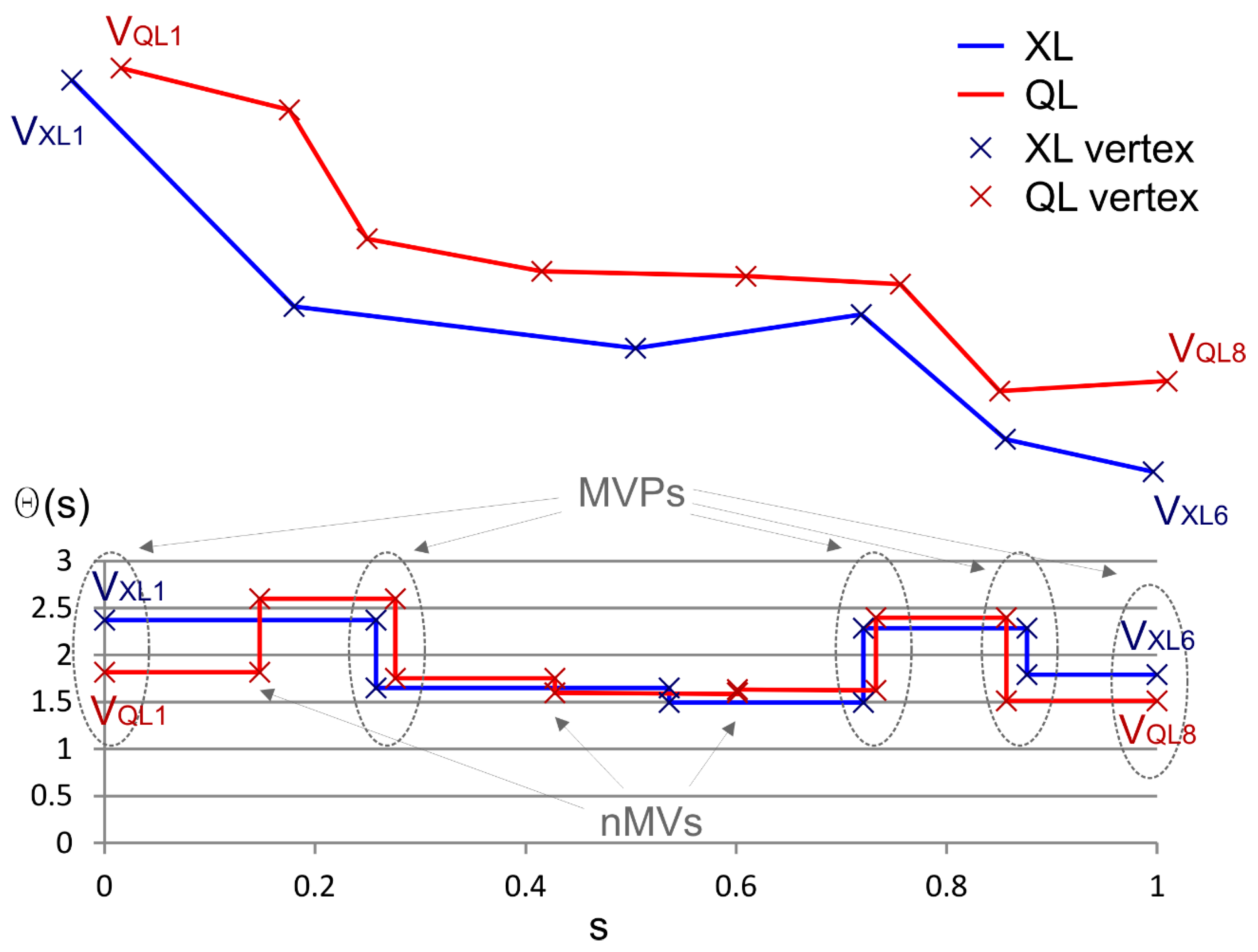
In the example shown in Figure 6, five pairs of vertexes are detected as Matching Vertexes Pairs (MVPs) and are considered as homologous: VQL1-VXL1, VQL3-VXL2, VQL6-VXL4, VQL7-VXL5, and VQL8-VXL6. The vertexes of XL, defined as Matching Vertexes (MVs), will compose AL (VAL1, VAL3, VAL6, VAL7, and VAL8), but we also have to determine the positions in AL of the rest of the vertexes of QL, which have not found homologous relationships in XL (VQL2, VQL4, and VQL5 in Figure 6, for example) in order to complete AL. The procedure of determining the non-matching vertexes (nMV) is based on an interpolation between each consecutive MV in XL based on the length (s) of the implicated nMV vertex in QL. In the example shown in Figure 6, VAL2 is determined by the interpolation of the length of VQL2 between the adjacent MV of QL (VQL1 and VQL3) on the section of the XL line between the homologous MV of XL (VXL1 and VXL2). After all vertexes of QL have established a unique relationship, an ALi is obtained (Figure 4). The adjustment of ALi to XL is checked while using the VIM (XL vs ALi). The application of different values to the parameters will generate alternative ALi. Accordingly, the process of obtaining AL is repeated using all possible combinations for each parameter, taking values from a determined range. The selection of the definitive AL is based on the minimum value of mean displacement obtained using VIM (XL vs each ALi).
- 3.
- Apply the VIM-V: Once we have two lines that are composed of the same number of vertexes and those vertexes are considered as homologous, the VIM-V method is applied from QL to AL, obtaining a mean displacement vector for the line.
- 4.
- Level of adjustment: The quality of the mean displacement vector obtained is directly related to the adjustment of the AL to XL. There are two metrics that can be used to analyze this level of adjustment: The mean displacement value of AL with respect to XL (previously obtained using VIM); and, the ratio between the lengths of the XL and the AL. In this context, we can use these metrics in order to filter those results that will be considered in the assessment.
- 5.
- Results of the assessment: The displacement vectors of a set of lines that have met the requirements imposed in the previous stage are used in the final assessment.
3. Results and Discussion
Once the QL and the XL datasets cases were obtained and combined, as was described in the methodology section, the proposed method was applied using a software application that was developed in JavaTM for this purpose. The results of the implementation of the proposed method to the sets of lines described in the previous stage provided one mean displacement vector by line and consequently a derived mean displacement vector for the total dataset for each morphology class (CL1–CL5). This supposes the obtaining of 146,320 values of displacement ((29 + 30) perturbed types × 5 CL classes × 496 lines). In order to check the method, these values were compared to the real mean displacements (by lines and totally) that were obtained from the particular perturbation applied to the vertexes. The differences between the displacements applied to the vertexes (calculated using the coordinates of the original and perturbed vertexes) and those that were derived from VIM-V were lower than 1.5 cm in all cases.
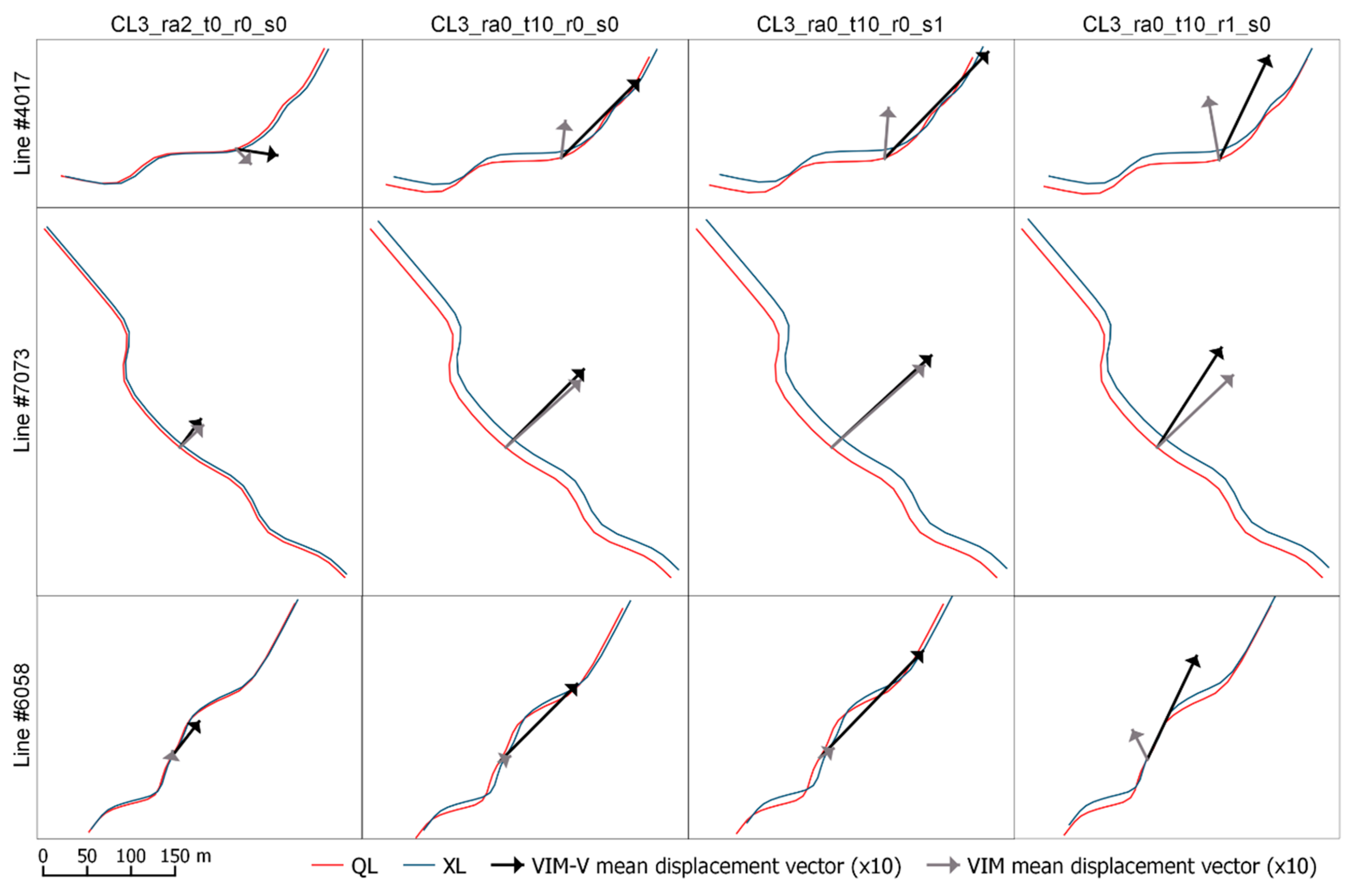
In addition to these general results, we also analysed the results that were obtained for some specific lines as an example (Figure 7). The VIM-V displacement vectors were compared to those that were obtained using VIM [18] for three lines of the CL3 class (#4017, #7073, and #6058 rows in Figure 7) with random and systematic perturbations. More specifically, in Figure 7 columns show different perturbations (ra2_t0_r0_s0, ra0_t10_r0_s0, ra0_t10_r0_s1, and ra0_t10_r1_s0), which correspond to random, translation, scaling and rotation, respectively. All cases show that VIM vectors are lower than VIM-V. However, this reduction is greater when the direction of the line is more coincident with the displacement applied (lines #4017 and #6058), while the vectors are more similar in cases of displacements perpendicular to the direction of the line (line #7073). VIM-V also shows great efficiency in detecting scaling and rotations.
The application of the method that is proposed in this study was based on a large set of lines with known perturbations. This aspect contributes to providing reliability to the results that were obtained and consequently to the method proposed. The use of five morphology classes added forcefulness to this application because of the possibility of analysing lines classified by their sinuosity.
The results of the application of the proposed method have demonstrated its ability to detect real displacements applied to the vertices of a line, including all types of perturbations (random, systematic, and combined), even when the direction of displacements applied is coincident with the direction of the line. More specifically, the results showed that the mean differences between the displacements applied and the displacements detected were lower than 1.5 centimetres. These results confirm the convenience of using the VIM-V method to analyse these displacements, even at large scales. The comparison of results from VIM-V and VIM on several specific lines confirmed that the VIM method usually estimates reduced values of displacements because of the behaviour of the lines themselves. This reduction is greater when there is greater coincidence between the directions of the lines and the displacement applied.
4. Conclusions
The results of the methods for assessing the positional accuracy of linear elements can hide bias displacements when these spatial differences are displayed in the same direction of the line. The difference can be important depending on the geometry of the line, which can hide some displacements, obtaining erroneous results when we try to estimate real displacements.
In this study, we have developed a new method in order to resolve this issue in cases where the determination of the real displacement suffered by lines is required. We consider the shape of both lines (to be assessed and assessor) by means of homologous vertexes in order to obtain an accurate result. Thus, the use of homologous vertexes is the main contribution of this new approach. In this sense, the problem is reduced to calculating the actual displacements between homologous vertexes. The homologous vertex determination can be performed by any of the existing algorithms or that developed in this study.
The VIM-V method consists of the determination of the mean displacement vector derived from every individual vector obtained between two homologous vertexes and weighted by the length of the segments adjacent to that vertex.
The application of the proposed method has allowed us to test its efficiency. We used a large number of lines that were affected with known displacements. The design of the experiment carried out has allowed for the application of most types of displacements (random and systematic) individually or combined to several datasets of lines characterized by five morphology classes, depending on their sinuosity. Accordingly, we consider that the method has been contrasted sufficiently, showing a high level of reliability in the results.
Future research will focus on the increase of the dataset to other elements represented by lines (e.g., rivers). This update will improve datasets that are available to researchers, such as MatchingLand.
Author Contributions
All authors conceived and designed the study, performed and analyzed the experiments and wrote the paper. All authors read and approved the manuscript.
Funding
The National Ministry of Economy and Competitiveness of Spain supported this work under the grant No. BIA2011-23271.
Acknowledgments
The authors thank the reviewers for their suggestions.
Conflicts of Interest
The authors declare no conflict of interest.
References
- Goodchild, M.F. Citizens as sensors: The world of volunteered geography. GeoJournal 2007, 69, 211–221. [Google Scholar] [CrossRef]
- MacEachren, A.M. Compactness of geographic shape: Comparison and evaluation of measures. Geogr. Ann. Ser. B Hum. Geogr. 1985, 67, 53–67. [Google Scholar] [CrossRef]
- Wentz, E.A. Shape analysis in GIS. In Proceedings of the Auto-Carto 13, Seattle, WA, USA, 7–10 April 1997. [Google Scholar]
- Arkin, E.M.; Chew, L.P.; Huttenlocher, D.P.; Kedem, K.; Mitchell, J.S.B. An efficiently computable metric for comparing polygonal shapes. IEEE Trans. Pattern Anal. 1991, 13, 209–216. [Google Scholar] [CrossRef] [Green Version]
- Perkal, J. On epsilon length. Bull. Acad. Pol. Sci. 1956, 4, 399–403. [Google Scholar]
- Chrisman, N.R. A theory of cartographic error and its measurement in digital bases. In Proceedings of the Fifth International Symposium on Computer-Assisted Cartography, Crystal City, VI, USA, 22–28 August 1982; Foreman, J., Ed.; pp. 159–168. [Google Scholar]
- Blakemore, M. Generalisation and error in spatial data bases. Cartographica 1984, 21, 131–139. [Google Scholar] [CrossRef]
- Caspary, W.; Scheuring, R. Positional accuracy in spatial databases. Comput. Environ. Urban Syst. 1993, 17, 103–110. [Google Scholar] [CrossRef]
- Shi, W.; Liu, W. A stochastic process-based model for the positional error of line segments in GIS. Int. J. Geogr. Inf. Sci. 2000, 14, 51–66. [Google Scholar] [CrossRef]
- Heuvelink, G.; Brown, J.D.; Van Loon, E.E. A Probabilistic Framework for Representing and Simulating Uncertain Environmental Variables. Int. J. Geogr. Inf. Sci. 2007, 21, 497–513. [Google Scholar] [CrossRef]
- Wu, H.S.; Liu, Z.L. Simulation and Model Validation of Positional Uncertainty of Line Feature on Manual Digitizing a Map. In The International Archives of the Photogrammetry, Remote Sensing and Spatial Information Sciences; Chen, J., Jiang, J., Kainz, W., Eds.; The International Society of Photogrammetry and Remote Sensing (ISPRS): Beijing, China, 2008; Volume XXXVII, Part B2; pp. 843–848. [Google Scholar]
- Gil de la Vega, P.; Ariza-López, F.J.; Mozas-Calvache, A.T. Models for positional accuracy assessment of linear features: 2D and 3D cases. Surv. Rev. 2016, 48, 347–360. [Google Scholar] [CrossRef]
- McMaster, R.B. A statistical analysis of mathematical measures for linear simplification. Am. Cartogr. 1986, 13, 103–116. [Google Scholar] [CrossRef]
- Jasinski, M.J. The Comparison of Complexity Measuresfor Cartographic Lines. Technical Report 90-1; National Center for Geographic Information and Analysis: Buffalo, NY, USA, 1990. [Google Scholar]
- Lawford, G.J. Examination of the Positional Accuracy of Linear Features. J. Spat. Sci. 2010, 55, 219–235. [Google Scholar] [CrossRef]
- Abbas, I.; Grussenmeyer, P.; Hottier, P. Contrôle de la planimétrie d’une base de données vectorielles: Une nouvelle méthode basée sur la distance de Haussdorff: La méthode du contrôle linéaire. Bull. SFPT 1995, 137, 6–11. [Google Scholar]
- Mozas, A.T.; Ariza, F.J. Methodology for positional quality control in cartography using linear features. Cartogr. J. 2010, 47, 371–378. [Google Scholar] [CrossRef]
- Mozas-Calvache, A.T.; Ariza-López, F.J. New method for positional quality control in cartography based on lines. A comparative study of methodologies. Int. J. Geogr. Inf. Sci. 2011, 25, 1681–1695. [Google Scholar] [CrossRef]
- Mozas-Calvache, A.; Ariza-López, F.J. Adapting 2D positional control methodologies based on linear elements to 3D. Surv. Rev. 2015, 47, 195–201. [Google Scholar] [CrossRef]
- Goodchild, M.F.; Hunter, G.J. A simple positional accuracy measure for linear features. Int. J. Geogr. Inf. Sci. 1997, 11, 299–306. [Google Scholar] [CrossRef]
- Tveite, H.; Langaas, S. An accuracy assessment method for geographical line data sets based on buffering. Int. J. Geogr. Inf. Sci. 1999, 13, 27–47. [Google Scholar] [CrossRef] [Green Version]
- Asakura, K.; Takeuchi, M.; Watanabe, T. A Map Matching Algorithm for Sharing Map Information among Refugees in Disaster Areas. In Intelligent Interactive Multimedia: Systems and Services; Watanabe, T., Watada, J., Takahashi, N., Howlett, R., Jain, L., Eds.; Springer: Berlin/Heidelberg, Germany, 2012; pp. 22–31. [Google Scholar] [CrossRef]
- Xi, L.; Liu, Q.; Li, M.; Liu, Z. Map matching algorithm and its application. In Proceedings of the International Conference on Intelligent Systems and Knowledge Engineering, Chengdu, China, 15–16 October 2007; Atlantis Press: Paris, France, 2007; pp. 1–7. [Google Scholar] [CrossRef]
- Quddus, M.A.; Ochieng, W.Y.; Noland, R.B. Current map-matching algorithms for transport applications: State-of-the art and future research directions. Transp. Res. C-Emererg. 2007, 15, 312–328. [Google Scholar] [CrossRef] [Green Version]
- Kieler, B.; Huang, W.; Haunert, J.H.; Jiang, J. Matching River Datasets of Different Scales. In Advances in GIScience; Sester, M., Bernard, L., Paelke, V., Eds.; Springer: Berlin/Heidelberg, Germany, 2010; pp. 135–154. [Google Scholar] [CrossRef]
- Reinoso, J.F. A priori horizontal displacement (HD) estimation of hydrological features when versioned DEMs are used. J. Hydrol. 2010, 384, 130–141. [Google Scholar] [CrossRef]
- Xavier, E.; Ariza-López, F.J.; Ureña-Cámara, M.A. A Survey of Measures and Methods for Matching Geospatial Vector Datasets. ACM Comput. Surv. 2016, 49, 1–34. [Google Scholar] [CrossRef]
- Mozas-Calvache, A.T.; Ariza-López, F.J. Detection of systematic displacements in spatial databases using linear elements. Cartogr. Geogr. Inf. Sci. 2014, 41, 309–322. [Google Scholar] [CrossRef]
- Xavier, E.; Ariza-López, F.J.; Ureña-Cámara, M.A. MatchingLand, geospatial data testbed for the assessment of matching methods. Sci. Data 2017, 4, 170180. [Google Scholar] [CrossRef] [PubMed] [Green Version]
- Montgomery, D.C.; Runger, G.C. Applied Statistics and Probability for Engineers; John Wiley & Sons: Hoboken, NJ, USA, 2010; ISBN 978-0470053041. [Google Scholar]
- Ariza-López, F.J.; García-Balboa, J.L. Generalization-oriented road line segmentation by means of an artificial neural network applied over a moving window. Pattern Recognit. 2008, 41, 1593–1609. [Google Scholar] [CrossRef]
Figure 1.
Example of Vertex Influence Method (VIM) [18].
Figure 1.
Example of Vertex Influence Method (VIM) [18].

Figure 2.
Examples of displacements applied to a segment.

Figure 3.
Datasets of lines used in the application: (a) general view; (b) Zoom view showing the 5 morphology classes (CL1 to CL5) for a sample of several lines.
Figure 3.
Datasets of lines used in the application: (a) general view; (b) Zoom view showing the 5 morphology classes (CL1 to CL5) for a sample of several lines.

Figure 4.
The Vertex Influence Method by Vertexes (VIM-V) approach proposed in this study.

Figure 5.
Method proposed in this study.

Figure 6.
Turning functions of XL and QL based on Arkin et al. [4] and Matching Vertexes Pair (MVP) determination.
Figure 6.
Turning functions of XL and QL based on Arkin et al. [4] and Matching Vertexes Pair (MVP) determination.

Figure 7.
Examples of VIM-V and VIM displacement vectors on specific lines (vectors are multiplied by 10).
Figure 7.
Examples of VIM-V and VIM displacement vectors on specific lines (vectors are multiplied by 10).


Table 1.
Main characteristics of the datasets of lines.
| Class | Number of Lines | Total Length (m) | Minimum Length (m) | Maximum Length (m) | Number of Vertexes (n) | Mean Segment (m) |
|---|---|---|---|---|---|---|
| CL1 | 496 | 183,736.15 | 4.48 | 3614.79 | 6555 | 30.33 |
| CL2 | 496 | 186,386.59 | 4.48 | 3636.38 | 13,813 | 13.99 |
| CL3 | 496 | 190,659.09 | 4.48 | 3754.90 | 11,718 | 16.99 |
| CL4 | 496 | 193,552.72 | 4.48 | 3614.79 | 9765 | 20.88 |
| CL5 | 496 | 194,166.64 | 4.48 | 3614.79 | 9209 | 22.28 |
Table 2.
Perturbed set of lines (XL) used in this application for CL1 to CL5 classes: random or systematic perturbations obtained from Matching Land.
Table 2.
Perturbed set of lines (XL) used in this application for CL1 to CL5 classes: random or systematic perturbations obtained from Matching Land.
| Perturbed Sets (XL) 1 | Random (m) | Translation (m) | Rotation (rad) | Scaling |
|---|---|---|---|---|
| ra1_t0_r0_s0 | 5 | - | - | - |
| ra2_t0_r0_s0 | 12.5 | - | - | - |
| ra3_t0_r0_s0 | 25 | - | - | - |
| ra0_t0_r0_s1 | - | - | - | 1.00052 |
| ra0_t0_r0_s2 | - | - | - | 0.999478 |
| ra0_t0_r1_s0 | - | - | 0.000521513 | - |
| ra0_t0_r1_s1 | - | - | 0.000521513 | 1.00052 |
| ra0_t0_r1_s2 | - | - | 0.000521513 | 0.999478 |
| ra0_t0_r2_s0 | - | - | 0.000521513 | - |
| ra0_t0_r2_s1 | - | - | 0.000521513 | 1.00052 |
| ra0_t0_r2_s2 | - | - | 0.000521513 | 0.999478 |
| ra0_t2_r0_s0 | - | 5 | - | - |
| ra0_t2_r0_s1 | - | 5 | - | 1.00052 |
| ra0_t2_r0_s2 | - | 5 | - | 0.999478 |
| ra0_t2_r1_s0 | - | 5 | 0.000521513 | - |
| ra0_t2_r1_s1 | - | 5 | 0.000521513 | 1.00052 |
| ra0_t2_r1_s2 | - | 5 | 0.000521513 | 0.999478 |
| ra0_t2_r2_s0 | - | 5 | 0.000521513 | - |
| ra0_t2_r2_s1 | - | 5 | 0.000521513 | 1.00052 |
| ra0_t2_r2_s2 | - | 5 | 0.000521513 | 0.999478 |
| ra0_t10_r0_s0 | - | 12.5 | - | - |
| ra0_t10_r0_s1 | - | 12.5 | - | 1.00052 |
| ra0_t10_r0_s2 | - | 12.5 | - | 0.999478 |
| ra0_t10_r1_s0 | - | 12.5 | 0.000521513 | - |
| ra0_t10_r1_s1 | - | 12.5 | 0.000521513 | 1.00052 |
| ra0_t10_r1_s2 | - | 12.5 | 0.000521513 | 0.999478 |
| ra0_t10_r2_s0 | - | 12.5 | 0.000521513 | - |
| ra0_t10_r2_s1 | - | 12.5 | 0.000521513 | 1.00052 |
| ra0_t10_r2_s2 | - | 12.5 | 0.000521513 | 0.999478 |
1 The key for the perturbed sets is as follows: ra = random perturbation, t = systematic translation, r = rotation and s = scaling. For example the case ra0_t10_r2_s1 means: ra0 = no random perturbation, t10 = translation case 10, r2 = rotation case 2 and s1 = scaling case 1.
Table 3.
Perturbed set of lines used in this application for CL1 to CL5 classes: combined random and systematic perturbations.
Table 3.
Perturbed set of lines used in this application for CL1 to CL5 classes: combined random and systematic perturbations.
| Perturbed SETS (XL) 1 | Random (m) | Translation (m) | Rotation (rad) | Scaling |
|---|---|---|---|---|
| ra1_t0_r1_s0 | 5 | - | 0.000521513 | - |
| ra1_t0_r0_s1 | 5 | - | - | 1.00052 |
| ra1_t2_r0_s0 | 5 | 5 | - | - |
| ra1_t2_r1_s0 | 5 | 5 | 0.000521513 | - |
| ra1_t2_r0_s1 | 5 | 5 | - | 1.00052 |
| ra1_t2_r1_s1 | 5 | 5 | 0.000521513 | 1.00052 |
| ra1_t10_r0_s0 | 5 | 12.5 | - | - |
| ra1_t10_r1_s0 | 5 | 12.5 | 0.000521513 | - |
| ra1_t10_r0_s1 | 5 | 12.5 | - | 1.00052 |
| ra1_t10_r1_s1 | 5 | 12.5 | 0.000521513 | 1.00052 |
| ra2_t0_r1_s0 | 12.5 | - | 0.000521513 | - |
| ra2_t0_r0_s1 | 12.5 | - | - | 1.00052 |
| ra2_t2_r0_s0 | 12.5 | 5 | - | - |
| ra2_t2_r1_s0 | 12.5 | 5 | 0.000521513 | - |
| ra2_t2_r0_s1 | 12.5 | 5 | - | 1.00052 |
| ra2_t2_r1_s1 | 12.5 | 5 | 0.000521513 | 1.00052 |
| ra2_t10_r0_s0 | 12.5 | 12.5 | - | - |
| ra2_t10_r1_s0 | 12.5 | 12.5 | 0.000521513 | - |
| ra2_t10_r0_s1 | 12.5 | 12.5 | - | 1.00052 |
| ra2_t10_r1_s1 | 12.5 | 12.5 | 0.000521513 | 1.00052 |
| ra3_t0_r1_s0 | 25 | - | 0.000521513 | - |
| ra3_t0_r0_s1 | 25 | - | - | 1.00052 |
| ra3_t2_r0_s0 | 25 | 5 | - | - |
| ra3_t2_r1_s0 | 25 | 5 | 0.000521513 | - |
| ra3_t2_r0_s1 | 25 | 5 | - | 1.00052 |
| ra3_t2_r1_s1 | 25 | 5 | 0.000521513 | 1.00052 |
| ra3_t10_r0_s0 | 25 | 12.5 | - | - |
| ra3_t10_r1_s0 | 25 | 12.5 | 0.000521513 | - |
| ra3_t10_r0_s1 | 25 | 12.5 | - | 1.00052 |
1 The key for the perturbed sets is as follows: ra = random perturbation, t = systematic translation, r = rotation and s = scaling. For example, the case ra1_t10_r0_s0 means: ra = random perturbation case 1, t10 = translation case 10, r0 = no rotation and s0= no scaling.
Table 4.
Values of parameters used in this application.
| Parameter | Minimum | Maximum | Step | Cases |
|---|---|---|---|---|
| ps | 10% of the mean segment | 50% of the mean segment | 10% of the mean segment | 5 |
| pΘ | 0.0157 rad | 0.3142 rad | 0.0785 rad | 5 |
| pdΘ | 0.1571 rad | 0.4712 rad | 0.1571 rad | 4 |
© 2018 by the authors. Licensee MDPI, Basel, Switzerland. This article is an open access article distributed under the terms and conditions of the Creative Commons Attribution (CC BY) license (http://creativecommons.org/licenses/by/4.0/).
Share and Cite
MDPI and ACS Style
Mozas-Calvache, A.T.; Ariza-López, F.J. Assessment of Displacements of Linestrings Based on Homologous Vertexes. ISPRS Int. J. Geo-Inf. 2018, 7, 473. https://0-doi-org.brum.beds.ac.uk/10.3390/ijgi7120473
AMA Style
Mozas-Calvache AT, Ariza-López FJ. Assessment of Displacements of Linestrings Based on Homologous Vertexes. ISPRS International Journal of Geo-Information. 2018; 7(12):473. https://0-doi-org.brum.beds.ac.uk/10.3390/ijgi7120473
Chicago/Turabian StyleMozas-Calvache, Antonio Tomás, and Francisco Javier Ariza-López. 2018. "Assessment of Displacements of Linestrings Based on Homologous Vertexes" ISPRS International Journal of Geo-Information 7, no. 12: 473. https://0-doi-org.brum.beds.ac.uk/10.3390/ijgi7120473
Note that from the first issue of 2016, this journal uses article numbers instead of page numbers. See further details here.