On the Statistical Distribution of the Nonzero Spatial Autocorrelation Parameter in a Simultaneous Autoregressive Model

Abstract

This paper focuses on the spatial autocorrelation parameter $\rho$ of the simultaneous autoregressive model, and furnishes its sampling distribution for nonzero values, for two regular square (rook and queen) tessellations as well as a hexagonal case with rook connectivity, using Monte Carlo simulation experiments with a large sample size. The regular square lattice directly relates to increasingly used, remotely sensed images, whereas the regular hexagonal configuration is frequently used in sampling and aggregation situations. Results suggest an asymptotic normal distribution for estimated $\rho$. More specifically, this paper posits functions between $\rho$ and its variance for three adjacency structures, which makes hypothesis testing implementable and furnishes an easily-computed version of the asymptotic variance for $\rho$ at zero for each configuration. In addition, it also presents three examples, where the first employed a simulated dataset for a zero spatial autocorrelation case, and the other two used two empirical datasets—of these, one is a census block dataset for Wuhan (with a Moran coefficient of 0.53, allowing a null hypothesis of, e.g., $\rho =0.7$) to illustrate a moderate spatial autocorrelation case, and the other is a remotely sensed image of the Yellow Mountain region, China (with a Moran coefficient of 0.91, allowing a null hypothesis of, e.g., $\rho =0.95$) to illustrate a high spatial autocorrelation case.

1. Introduction

Spatial autocorrelation (SA) is a common phenomenon of spatial data analyses, where there is a common naive hypothesis that SA is zero (e.g., [1,2,3]) for datasets involving, for example, georeferenced demographic, social economic, and remotely sensed image variables. A more reasonable postulate would be nonzero SA. Gotelli and Ulrich [4] (p. 171) also pointed out that one of the important challenges in null modeling testing in ecology is “creating null models that perform well with … varying degrees of SA in species occurrence data”. This is a challenge that is not unique to ecology. A main problem hindering the positing of a nonzero SA hypothesis, or varying degrees of SA, is the unknown sampling distribution of the SA parameter, which may be denoted by $\rho$ of the simultaneous autoregressive (or SAR, which is called the “spatial error model” in spatial econometrics [5] (p. 5)) model in this paper. This parameter quantifies the degree of self-correlation in the error term (e.g., [6] (p. 42, which can be rewritten as Equation (1)); as when it deviates further from zero, its distribution becomes more skewed and peaked, and its variance decreases. 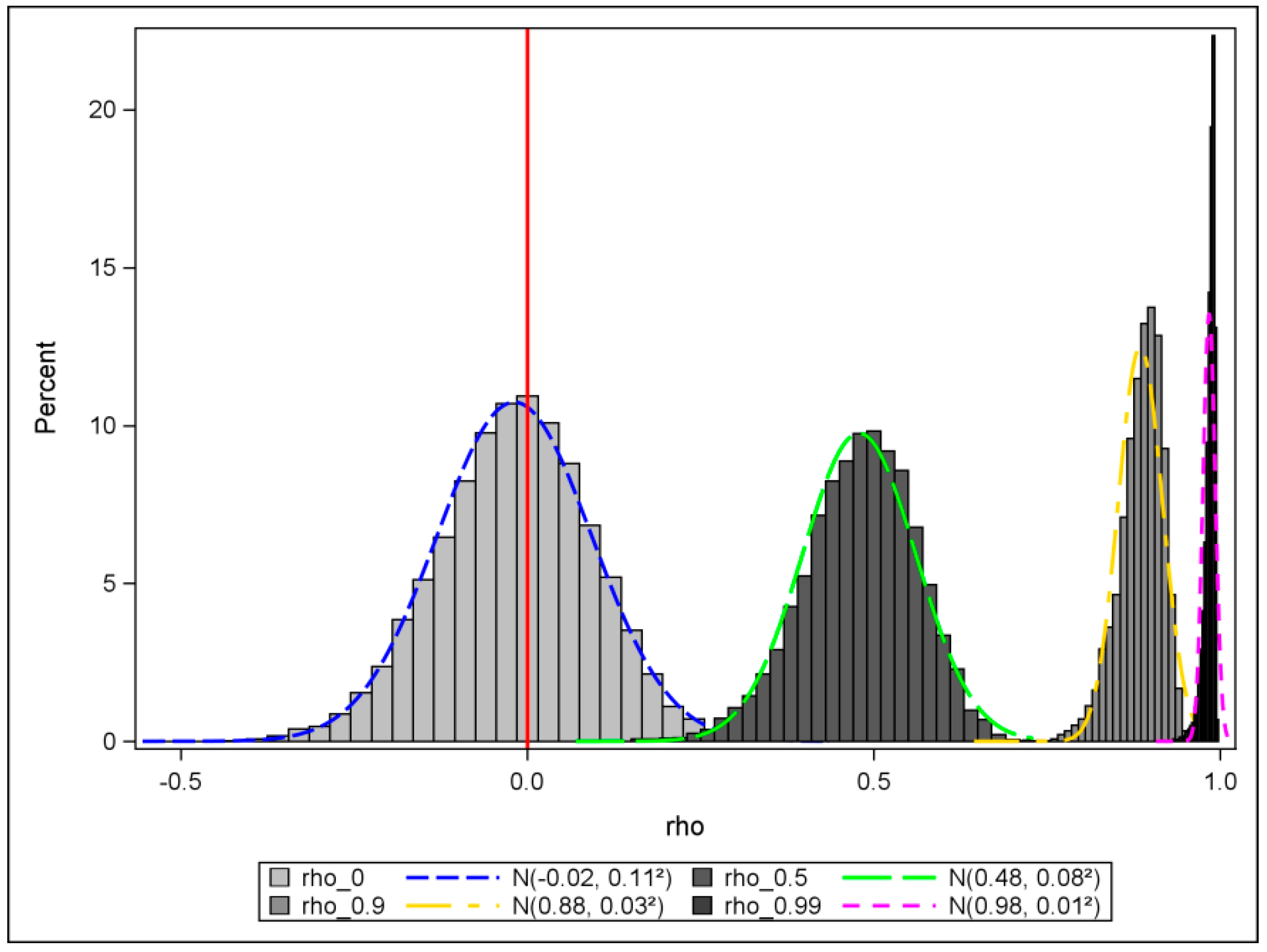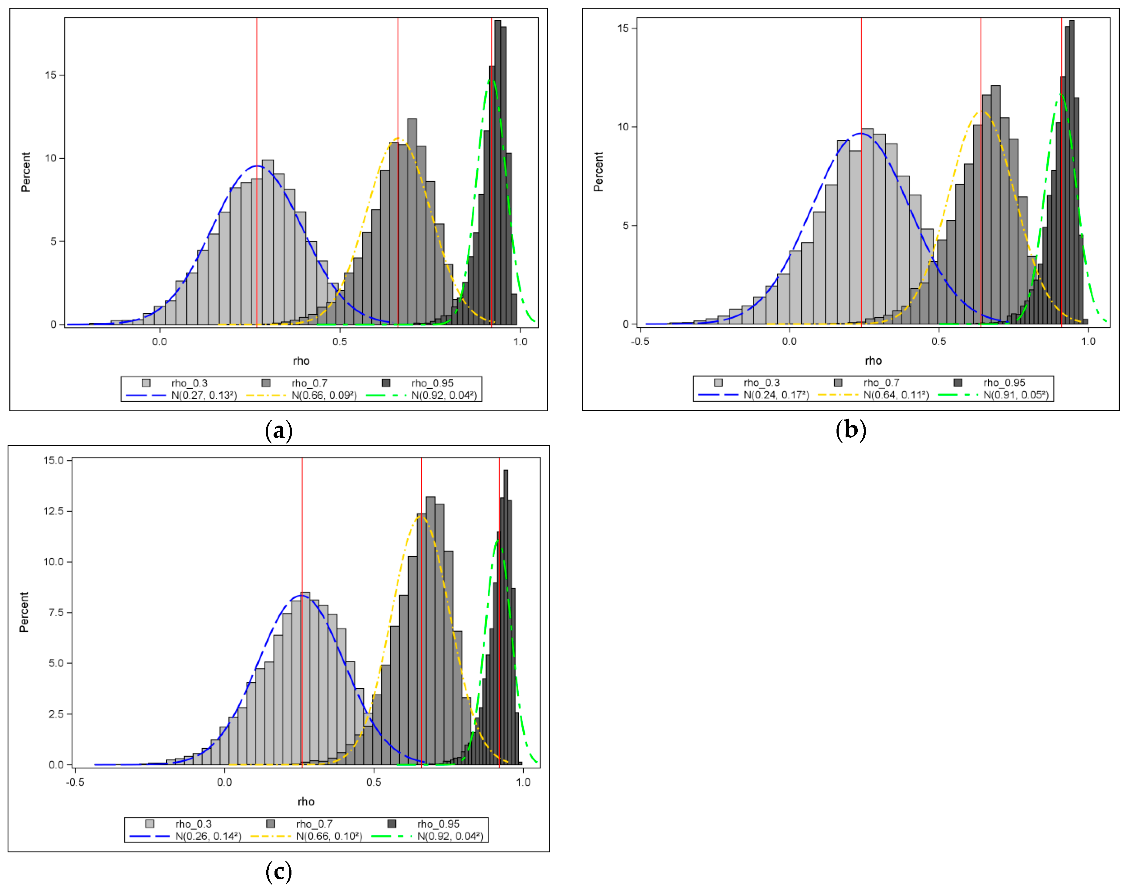Figure 1 shows this phenomenon, where its connectivity matrix comes from the Wuhan census block data that are employed in the moderate SA case. Four histograms with density curves for different $\rho$ values of 0, 0.5, 0.9, and 0.99 reveal that as $\rho$ increases, the distribution moves further from zero (see the red reference line perpendicular to the horizontal axis), and its shape becomes narrower.

To gain an understanding of the complications related to figuring out the sampling distribution of the test statistic under the nonzero hypothesis, it is always enlightening to look back to Pearson’s r (i.e., correlation coefficient) in standard statistics and the autocorrelation coefficient in time series models, because the SA coefficient resembles the “auto” version of the former, and extends the latter from a uni-direction (time dimension) to a multi-directions (space dimension) case. A parallel to what is commonly done in spatial scenarios is that a routine null hypothesis often sets the (auto)correlation coefficient to zero in classical statistics or time series (e.g., [7,8]). In order to test the nonzero correlation coefficient in standard statistics, a Fisher’s Z-transformation is used so that the transformed statistic is approximately normally distributed and its variance is stabilized (e.g., [9] (pp. 55–56); [10] (p. 487); [11]). However, for the original $\rho$, the distribution becomes skewed as $\rho$ approaches its extreme values. Fortunately, Provost [12] suggests closed-form representations of the density function and integer moments of the sample correlation coefficient to furnish a solution for the distribution problem. For time series autocorrelations, the research on a statistical distribution of a nonzero coefficient was developed from a more practical viewpoint. For example, Ames and Reiter [13] established the distribution of autocorrelation coefficients in economic time series by using empirical datasets so that hypothesis testing for the significance of (auto)correlation among economic variables could have “a more appropriate basis” (p. 638) than the null hypothesis on a basis of zero (auto)correlation. More recent literature [14] pertaining to this topic focused on the effect of the nonzero coefficient on the distribution of the Durbin-Watson test estimator. Similarly to the time series literature, studies on the distribution of the nonzero autocorrelation coefficient/parameter are rare in spatial statistics. One related work dates back to 1967, in which Mead [15] verified that the Fisher’s Z-transformation did not help to obtain a stabilized variance, and even its generalized form could only help in instances of a very small $\rho$ (i.e., 0, ±0.05, ±0.1). This earlier work provides evidence that the variance problem seems to be a major obstacle for establishing a sampling distribution for nonzero $\rho$. This paper furnishes a possible solution for this problem by representing the variance of $\widehat{\rho }$ as a function of $\rho$, and validates the asymptotic normality of this distribution through Monte Carlo simulation experiments. Moreover, it also establishes a function between $\rho$ and the Moran Coefficient (MC, also known as Moran’s I, [16]), which bridges the most widely used SA statistic and spatial autoregressive model.

This paper contributes to the literature by establishing properties of the sampling distribution of nonzero $\rho$, supplementing the asymptotic variance known for zero $\rho$ in a regression framework. Its results also pertain to the conditional autoregressive (CAR) model, which is called the conditionally specified Gaussian (CSG) in spatial econometrics [17] (pp. 197 and 201), as well as the autoregressive response (AR) model, which is called the spatial lag model in spatial econometrics [5] (p. 5). A SAR model can also be written as a CAR model (e.g., [18] (p. 149); [19] (p. 123); [20] (p. 68)), both SAR and AR are of second-order (i.e., they also specify spatial correlation in terms of neighbors of neighbors), and their pure SA versions with no independent variables are the same model. The focus is on the SAR here because it is the most commonly used specification in spatial statistics, and the SAR uses the row standardized spatial weights matrix $\mathit{W}$, not matrix $\mathit{C}$ (see Section 2).

It is also necessary to explain the motivation of this paper from a more general perspective. Because Cliff and Ord [21] systematically introduced hypothesis testing for the existence of SA latent in spatial data, SA-related research, in terms of both its theoretical and applied aspects, has flourished in a wide range of domains employing datasets with geographical or locational information. Sokal and Oden [22,23] introduced SA into biology, which inspired biologists to take SA into account in their work because most biological or ecological datasets are closely related to geographical locations. Legendre [24] constructed a paradigm for ecologists to describe and test for SA, as well as to introduce spatial structure into ecological models. Other fields dealing with SA include, for example, spatial epidemiology (see [25] for a thorough overview), spatial econometrics (e.g., [26]), and urban planning (e.g., [27]), which often use Geographical Information Science (GIS, [28]) methods or tools. In all of these domains, testing the existence or presence of SA is a solved problem, where the next question which naturally arises is how the degree of SA could be tested. This paper furnishes an answer to this question.

This article consists of five sections. Section 2 presents model specification and parameter estimation. Section 3 furnishes the sampling distribution of the SA parameter estimate. Section 4 gives one simulated example for zero SA by setting the null hypothesis to be ${\rho }_0=0$, as well as two empirical examples. Empirical analyses from over the years disclose that most socio-economic/demographic attributes have a degree of correlation ranging from 0.4 to 0.6, which indicates a relevant range for $\rho$ within 0.65 to 0.85 [29]; thus, a moderate SA case sets the null hypothesis as ${\rho }_0=0.7$, whereas a strong SA case sets the null hypothesis as ${\rho }_0=0.95$. Section 5 presents conclusions and discussion. There are also appendices with some supplementary materials.

2. Model Specification and Parameter Estimation

This paper focuses on the SAR model and its SA parameter $\rho$. The first use of the word simultaneous as a descriptor of an autoregressive model was by Whittle [30], whose seminal article introduced an expression known as the SAR model for two-dimensional stationary processes. Concomitantly with the development of spatial statistics, the SAR model was frequently used by geographers, econometricians, ecologists, and other spatial researchers as one of the very popular specifications for describing georeferenced data.

This SAR model is specified as follows:

$$\mathit{Y}=\rho \mathit{W}\mathit{Y}+\left(\mathit{I}-\rho \mathit{W}\right)\mathit{X}\mathit{\beta }+\mathit{\epsilon },$$

(1)

where $\mathit{Y}$ is a response variable whose realizations $y_1, y_2, \cdots , y_n$ can be observations of a geographic attribute (e.g., average house price) distributed across $n$ regions, $\rho$ is a SA parameter, $\mathit{W}$ is a stochastic version (row standardized) of the n-by-n ($n^2$ entries) binary contiguity matrix $\mathit{C}$ (the entry of the ith row and jth column is 1 if region i and j are adjacent, and 0 otherwise)—both $\mathit{W}$ and $\mathit{C}$ reflect the spatial adjacency of a geographical phenomenon, $\mathit{I}$ is the n-by-n ($n^2$ entries) identity matrix, $\mathit{X}$ is a n-by-(m+1) ($nm+n$ entries) matrix with m explanatory variables (i.e., covariates) and one unit vector for the intercept, $\mathit{\beta }$ is a coefficient vector of the order (m+1)-by-1, and $\mathit{\epsilon }$ is a n-by-1 white-noise error term, which conforms to a standard multivariate normal distribution, $\mathit{\epsilon }~\mathit{M}\mathit{V}\mathit{N}\left(\mathbf{0}, {\sigma }^2\mathit{I}\right)$. In Equation (1), $\mathit{Y}$ appears on both sides of the equal sign, which is why the regression has the prefix, auto; when the equation is rewritten for individual observations, $n$ similar equations simultaneously appear.

Without loss of generality, $\mathit{X}$ can be void of covariates and contain only the intercept term, rendering a pure SA specification. Then, Equation (1) is reduced to:

$$\mathit{Y}=\rho \mathit{W}\mathit{Y}+{\beta }_0\left(\mathit{I}-\rho \mathit{W}\right)\mathbf{1}+\mathit{\epsilon },$$

(2)

where $\mathbf{1}$ is the n-by-1 vector of ones contained in matrix $\mathit{X}$. Equation (2) is also known as a pure SAR model, and is the specification employed in this paper. For the pure SAR specification, the error model and lag model are equivalent.

The parameters that need to be estimated in an SAR model are $\rho$, $\mathit{\beta }$ (for Equation (2), it is only ${\beta }_0$), and ${\sigma }^2$. As pointed out by Ord [31] (p. 122), the least squares estimator of $\rho$ is inconsistent, and even if this problem is revised by choosing an auxiliary matrix, the estimator is less efficient than a maximum likelihood estimator (MLE). Thus, ML estimation is a commonly used technique to estimate $\rho$ (e.g., [18,21]; [32]). Griffith [33] (pp. 176–177) provides explicit MLEs of these parameters, and furnishes an equivalent form for the MLE of $\rho$ that can be executed with the SAS code employed by this paper, and $\left|\rho \right|<1$ for square tessellation and the rook’s adjacency (for regular square queen, and hexagonal adjacencies, see §3.1). However, a well-known problem of the MLE is the computing burden of its logarithm determinant constituting its Jacobian term, i.e., $ln\left(\left|\mathit{I}-\rho \mathit{W}\right|\right)$, which becomes especially troublesome when a sample size becomes large. Griffith [34,35,36,37,38] (This work includes finding approximations of the Jacobian for regular, as well as irregular surface partitioning, exploring analytical or approximated expressions of eigenvalues of matrix $\mathit{C}$ and matrix $\mathit{W}$, and figuring out a simplified algorithm for calculating MLEs for massive sample sizes. In addition, this work establishes criteria to check the rationality of posited eigenvalue approximations, and to evaluate the Jacobian term approximations. Analyses summarized in this paper are based upon these contributions.) contributed some simplifications that reduced the computational burden of this factor. Another issue meriting attention here is the sampling variance of the model estimated $\rho$ (i.e., ${\widehat{\rho }}_{SAR}$, which is simplified to $\widehat{\rho }$ hereafter), because it measures the uncertainty or quantifies the precision of the ML estimate. Capturing how this variance changes is helpful for evaluating the efficiency of the estimator; in addition, it is always necessary to know at least the first- and the second-order central moments of a sampling distribution of a parameter estimator so that statistical inference can be conducted. Ord [31] (p. 124) suggests an asymptotic variance-covariance matrix of $\rho$ and ${\sigma }^2$, from which an expression of the asymptotic variance of $\widehat{\rho }$ can be obtained. This lays the foundation for exploring the analytical expression of the sampling variance of $\widehat{\rho }$ in this paper.

Another approach that can be used to estimate the SA parameter is the general method of moments (GMM) furnished by, among others, Kelejian and Prucha [39,40]. Walde et al. [41] present a thorough comparison between GMM- and MLE-based methods for very large-data spatial models, and suggest employing the former. A very important reason that led them to choose the GMM for large spatial data model estimation was that the GMM had a “directly computable” (p. 164) standard error of $\rho$, which is also implemented in a MLE framework in this paper. Section 3 describes this implementation in detail.

3. The Sampling Distribution of $\widehat{\mathit{\rho }}$

Before discussing the sampling distribution, it is necessary to introduce three surface partitionings on which all works of this paper are based: a regular square tessellation with rook connectivity (squares A and B are defined to be neighbors if they have a common edge), a regular square tessellation with queen connectivity (squares A and B are defined to be neighbors if they have a common edge or a common vertex), and a regular hexagonal tessellation with rook connectivity (hexagons A and B are defined to be neighbors if they have a common edge). There are definitely many types of geographical configurations, e.g., some theoretical types that have been discussed in [42], a more practical one that is used to construct grids for the earth’s surface (i.e., ISEA3H, [43]), a soccer ball-like configuration (i.e., a combination of hexagons and pentagons). However, only these three were employed, because the rook and queen are frequently-used criteria in many GIS and spatial data analysis-related software or packages (e.g., Esri ArcMap; spdep in R, [6]); moreover, these two adjacency schemes with a more regular square lattice relate to increasingly used, remotely sensed images. Also, a hexagonal configuration is often used in spatial sampling design [44] (pp. 24–25) and aggregation [43]. In summary, these three configurations are frequently used in practice, and many irregular lattices tend to have connectivities that are between a regular square and hexagon lattice (e.g., [42]). As shown in Figure 2, for a square tessellation, A has four neighbors for a rook adjacency, eight neighbors for a queen adjacency, and six neighbors for a hexagonal tessellation. Suppose there are $n$ observations of a geographical attribute distributed over one of these landscapes, considering the regularity, and let $n=P\times Q$, where $P$ is the number of rows, $Q$ is the number of columns, and the dimension of the connectivity matrix is n-by-n (i.e., $P^2\times Q^2$).

3.1. The Relationship between $\widehat{\rho }$ and the MC

In the literature, the most widely used statistic for quantifying SA is the MC. From a model perspective, $\rho$ is the parameter that has the same function as the MC. Although these two quantities are related, they are not equivalent, and thus should not be interchangeably used [1]. Establishing their explicit relationship quantitatively supports evaluation of the SA level latent in georeferenced data. Griffith [45] (pp. 33–34) points out that the relationship curve of $\widehat{\rho }$ against the MC is logistic (or sigmoid). This paper explores their relationship function further so that $\widehat{\rho }$ can be quantitatively described by the MC for the three surface partitionings discussed in this paper.

Suppose a geographical configuration has $n$ units. The estimates of $\mathsf{\rho }$ and the MC are closely related to matrix $\mathit{M}\mathit{C}\mathit{M}$, where $\mathit{C}$ is defined as done previously, $\mathit{M}$ is the projection matrix defined as $\mathit{I}-\mathit{J}/n$, and $\mathit{J}$ is a n-by-n matrix whose entries are all ones. Jong et al. [46] (pp. 21–22) demonstrated that $M{C}_{extreme}=\left(n/{\mathit{1}}^T\mathit{C}\mathit{1}\right){\lambda }_{extreme}$, which is indicative of the relationship between extreme MC values and extreme eigenvalues (denoted by $\lambda$) of $\mathit{M}\mathit{C}\mathit{M}$; in other words, the maximum eigenvalue corresponds to the maximum MC value, while the minimum eigenvalue corresponds to the minimum MC value. Because this equation restricts the feasible range of the MC, it is reasonable to generate a set of sample MC values by:

$$M{C}_i=\frac{n}{{\mathit{1}}^T\mathit{C}\mathit{1}}{\lambda }_i, i=1, 2, \dots , n.$$

(3)

Ordering the eigenvalues such that ${\lambda }_1\ge {\lambda }_2\ge \dots \ge {\lambda }_n$, the corresponding $\rho$ can be estimated for each by employing eigenvectors $\mathit{E}=\left(E_1, E_2, \dots , E_n\right)$ to replace $\mathit{Y}$ in Equation (2). That is:

$$E_i=\rho \mathit{W}{E}_i+{\beta }_0\left(\mathit{I}-\rho \mathit{W}\right)\mathit{1}+\mathit{\epsilon },i=1, 2, \dots , n.$$

(4)

The eigenvalue ${\lambda }_i$ and eigenvector $E_i \left(i=1, 2, \dots , n\right)$ correspond to the ith MC value, and this $E_i$ is also the response variable in the pure SAR model rendering an estimate for the ith $\rho$ value.

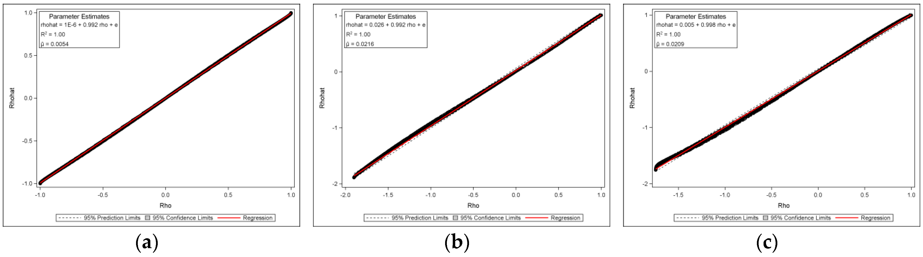
To explore the relationship between the MC and $\widehat{\rho }$, 14 groups of experiments with different sample sizes were conducted for the three configurations (i.e., regular square rook, regular square queen, and hexagonal cases), where $n$ ranged from 25 to 4900 (that is, $n=5\times 5, 10\times 10, \dots , 60\times 60, 65\times 65, 70\times 70$, where $P$ and $Q$ increase in increments of five). The theoretical relationship functions for different spatial configurations were defined, and the parameters were estimated.

Table 1. Theoretical functions for $\rho$ versus the Moran coefficient (MC).

Geographical Configurations	Function Forms	Parameter Estimates
Square rook	$\widehat{\rho } =\frac{a}{1+{\mathit{e}}^{b\ast MC+c}}+\frac{d}{{\lambda }_{min}}$	$\widehat{a}=2, \widehat{b}=-8, \widehat{c}=0, \widehat{d}=1$
Square queen	$\widehat{\rho } =\frac{a}{1+{\mathit{e}}^{{\left|MC+b\right|}^c}}+\frac{d}{{\lambda }_{min}}$	$\widehat{a}=5.8, \widehat{b}=-0.96, \widehat{c}=8, \widehat{d}=1$
Hexagonal		$\widehat{a}=5.5, \widehat{b}=-0.96, \widehat{c}=6.7, \widehat{d}=1$

summarizes the resulting expressions. The bold $\mathit{e}$ is the base of the natural logarithm, and ${\lambda }_{min}$ is the minimum eigenvalue of matrix $\mathit{W}$ (rook connectivity ${\lambda }_{min}$ is about −1, queen ${\lambda }_{min}$ is approximately −0.53, whereas ${\lambda }_{min}$ of the hexagonal tessellation is around −0.57).

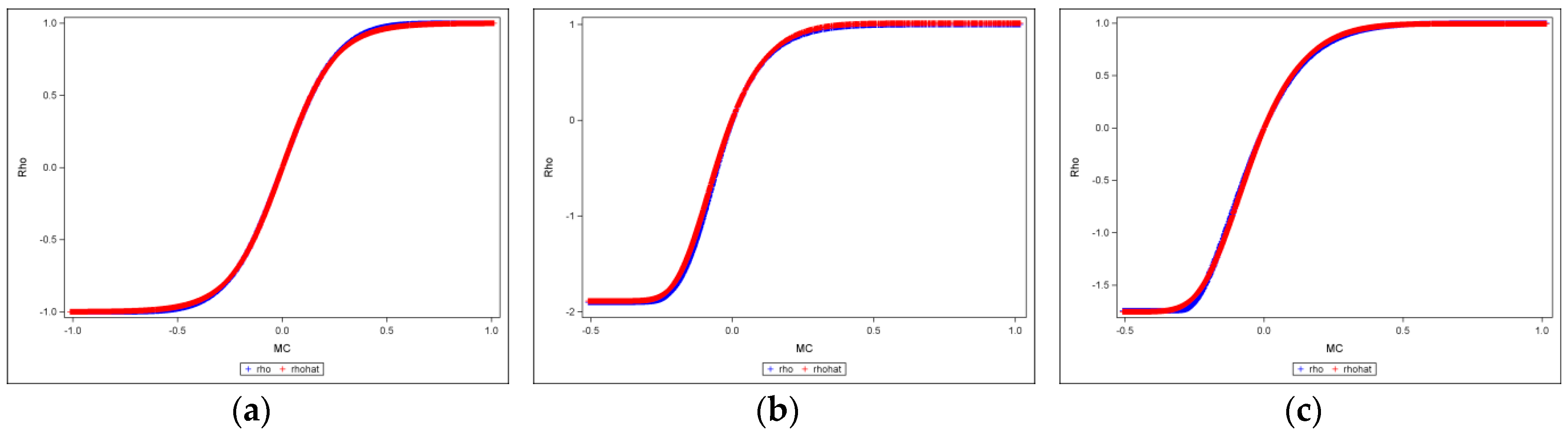
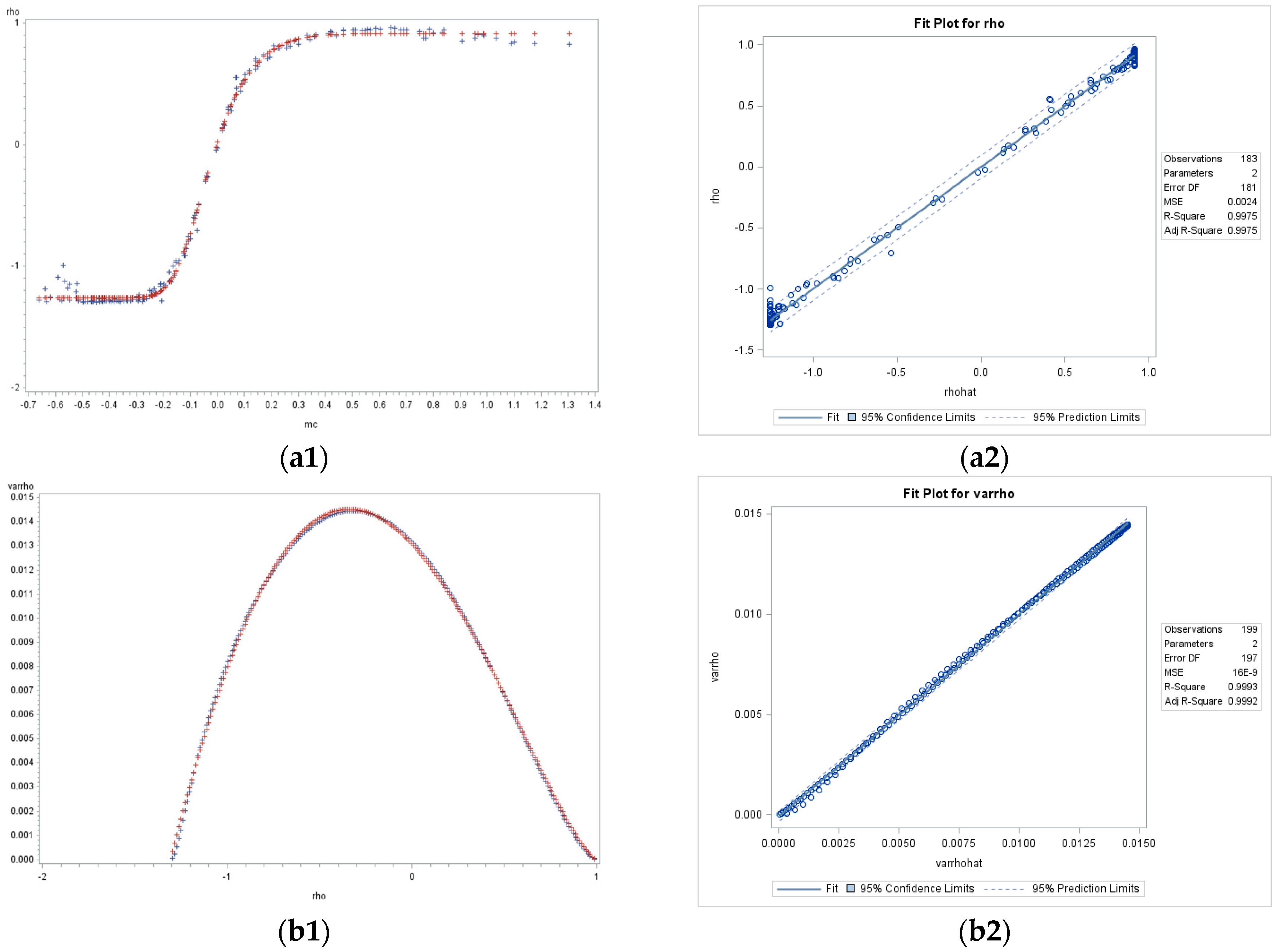
Figure 3 presents the selected fitted curves. This figure depicts the 70-by-70 ($n=4900$) configuration results for the square-rook, square-queen, and hexagonal cases. It presents the fitted curves (red), computed with the theoretical equation, superimposed on the observed data (blue), where the horizontal axis indicates the values of MC, and the vertical axis stands for the values of $\rho$ (here, $\rho$ denotes both the MC-estimated $\rho$ and the SAR-estimated $\rho$.); the regression lines of ${\widehat{\rho }}_{MC}$ (estimated by the functions of the MC in Table 1) versus $\widehat{\rho }$ are shown in Appendix A. Figure 3a reveals that for the square rook connectivity, the feasible range of the MC is approximately $\left[-1, 1\right]$, and the range of $\rho$ is $\left(-1,1\right)$. For the square queen (Figure 3b) and hexagonal (Figure 3c) cases, the MC is about $\left(-0.51, 1\right]$; $\rho$ is approximately $\left(-1.90, 1\right)$ and $\left(-1.74, 1\right)$, respectively (These intervals of $\rho$ verify the inequality ${\lambda }_{min}{}^{-1}<\widehat{\rho }<{\lambda }_{max}{}^{-1}$ (Ord, 1975, p124). While the most frequently used interval is $\left(-1,1\right)$ (refer to Section 2), intervals beyond this range can be transformed onto it.). These theoretical and original scatter plots match perfectly, with bivariate regression $R^2$s of nearly 1 (see Appendix A Figure A1).

3.2. The Sampling Variance of $\widehat{\rho }$

The sampling variance of $\widehat{\rho }$ is important because it quantifies the uncertainty with which $\rho$ is estimated. Ord [31] (p. 124) proposes the asymptotic variance-covariance matrix1 of $\rho$ and ${\sigma }^2$ (the value of diagonal entries of the variance-covariance matrix of error term $\mathit{\epsilon }$); for illustrative purposes, it is rewritten as:

$$V\left({\sigma }^2, \rho \right)={\sigma }^2{\left(\begin{array}{cc}\frac{n}{2{\sigma }^2}& tr\left(\mathit{B}\right)\\ tr\left(\mathit{B}\right)& {\sigma }^{2}tr\left({\mathit{B}}^T\mathit{B}\right)-\alpha {\sigma }^2\end{array}\right)}^{-1},$$

(5)

where $\mathit{B}={\left(I-\rho \mathit{W}\right)}^{-1}\mathit{W}, \alpha =-{\displaystyle \sum }_{i=1}^n{\lambda }_i^2/{\left(1-\rho {\lambda }_i\right)}^2$, ${\lambda }_i$ is the ith eigenvalue of matrix $\mathit{W}$, “tr” is the matrix trace operator, and superscript “T” is the matrix transpose operator. An asymptotic formula of the sampling variance of $\widehat{\rho }$ derived from Equation (5) by inverting the 2-by-2 matrix is $Var{\left(\widehat{\rho }\right)}_{asy}=\left(n/2\right)/\Delta$, where $∆=\left(n/2\right)tr\left({\mathit{B}}^T\mathit{B}\right)+\left(n/2\right){\displaystyle \sum }_{i=1}^n{\lambda }_i^2/{\left(1-\rho {\lambda }_i\right)}^2-{\left[tr\left(\mathit{B}\right)\right]}^2$. Hence, the variance expansion may be written as:

$$Var{(\widehat{\rho })}_{asy}=\frac{1}{tr({\mathit{W}}^T{(\mathit{I}-\rho {\mathit{W}}^T)}^{-1}{(\mathit{I}-\rho \mathit{W})}^{-1}\mathit{W})+{{\displaystyle \sum }}_{i=1}^n\frac{{\lambda }_i^2}{{(1-\rho {\lambda }_i)}^2}-\frac{2}{n}{\left[tr({(\mathit{I}-\rho \mathit{W})}^{-1}\mathit{W})\right]}^2}.$$

(6)

This equation is still not easy to compute because it involves (inverse) matrix operations, as well as eigenvalues. The following sub-sections present some simplifications which only consist of sample size (or number of observations) $n$, and the extreme eigenvalues of matrix $\mathit{W}$ (specifically, for zero SA cases, only $P$ and $Q$).

3.2.1. The Sampling Variance of $\widehat{\rho }$ at Zero

When $\rho =0$, Equation (6) becomes $Var{(\rho =0)}_{asy}=1/[tr({\mathit{W}}^T\mathit{W})+{\displaystyle \sum }_{i=1}^n{\lambda }_i^2]$. Because $\mathit{W}={\mathit{D}}^{-1}\mathit{C}$ ($\mathit{D}$. is a diagonal matrix whose $n$ diagonal entries are inverse row sums of matrix $\mathit{C}$), $\mathit{C}$ and ${\mathit{D}}^{-1}$ are square matrices, and $c_{ij}{}^2=c_{ij}$ because $\mathit{C}$ is binary, $tr({\mathit{W}}^T\mathit{W})=tr({\mathit{C}}^T{\mathit{D}}^{-1}{\mathit{D}}^{-1}\mathit{C})=tr({\mathit{C}}^2{\mathit{D}}^{-2})={\displaystyle \sum }_{i=1}^n[{\displaystyle \sum }_{j=1}^n{c}_{ij}{}^2/{({\displaystyle \sum }_{j=1}^n{c}_{ij})}^2]={\displaystyle \sum }_{i=1}^n(1/{\displaystyle \sum }_{j=1}^n{c}_{ij})$, then the asymptotic variance of $\rho$ at zero is:

$$Var{(\rho =0)}_{asy}=\frac{1}{{{\displaystyle \sum }}_{i=1}^n\frac{1}{{{\displaystyle \sum }}_{j=1}^n{c}_{ij}}+{{\displaystyle \sum }}_{i=1}^n{\lambda }_i^2}.$$

(7)

Table 2. Asymptotic variance of $\widehat{\rho }$ at zero for different surface partitionings.

Landscape	$\mathbf{Asymptotic} \mathbf{Variance} \mathbf{for} \mathit{\rho }=0.$
Square rook	$72/\left(36PQ+23P+23Q+36\right)$
Square queen	$2400/\left(600PQ+639P+639Q+794\right)$
Hexagonal	$180/\left(60PQ+55P+60Q+71\right)$

summarizes this variance for different surface partitionings; the formulae for summation of the inverse row sum of matrix $\mathit{C}$ and summation of squared eigenvalues of matrix $\mathit{W}$ are listed in Appendix B.

The expressions in Table 2 make Equation (7) extremely easy to compute, especially when the sample size is large. However, functions for $\rho$ at nonzero points are more complex. As has been argued by [15], the variance of the inter-plant competition coefficient (which is the sampling variance of $\rho$ that is discussed in this paper) cannot be stabilized by the Fisher Z-transformation, and even its generalized form only works on very weak spatial interactions (0, ±0.05, ±0.1) for three specific spatial configurations (i.e., 7, 12, and 19 hexagonally arranged points; see Figure 1 on p. 193). More recently, Griffith and Chun [47] emphasized that better quantifying the spatial variability of SA estimates is still a challenge. By exploring the distribution of the variance, this paper finds that the sampling variance of $\widehat{\rho }$ is a function of $\rho$ (which is implemented with $\widehat{\rho }$), which is depicted by a Beta distribution curve with equal parameters larger than 1.

3.2.2. The Sampling Variance of $\widehat{\rho }$ at Nonzero Values

To conduct the experiments, 30 groups of different sample sizes, ranging from 5-by-5 to 150-by-150 with $P$ and $Q$ increasing in increments of five, were employed; the sample size of each group was $P\times Q$. The SA parameter $\rho$ was uniformly sampled across its feasible ranges, namely, ${\lambda }_{min}{}^{-1}<\widehat{\rho }<{\lambda }_{max}{}^{-1}=1$, where $\lambda$ is an eigenvalue of matrix $\mathit{W}$. Theoretical functions of asymptotic variance versus $\widehat{\rho }$ are presented in

Table 3. Theoretical functions for asymptotic variance versus $\widehat{\rho }$.

Geographical Configurations	Function Forms	$\mathbf{Parameter} \mathbf{Estimates} \left({\mathit{R}}^2\right)$
Square rook	$Var{\left(\widehat{\rho }\right)}_{asy}=a\ast a_0\ast G^{b-1}$ $\ast {\left(1-G\right)}^{c-1}$	$\widehat{a}=\frac{17.9181}{n^{0.5395}}+6.7144 , \left(0.9999\right)$ $\widehat{b}=2.4, \widehat{c}=2.4$
Square queen		$\widehat{a}=\frac{32.4112}{n^{0.4482}}+6.4694, \left(0.9990\right)$ $\widehat{b}=\frac{2.0836}{n^{0.3519}}+2.1107,\left(0.9975\right)$ $\widehat{c}=\frac{1.0641}{n^{0.2982}}+2.2843, \left(0.9974\right)$
Hexagonal	$Var{\left(\widehat{\rho }\right)}_{asy}=a\ast a_0\ast G^{c\ast G+b-1}\ast {\left(1-G\right)}^{e\ast G+d-1}$	$\widehat{a}=\frac{30.1752}{n^{0.3065}}-0.0160, \left(0.9941\right)$ $\widehat{b}=\frac{3.0023}{n^{0.1121}}+0.5299, \left(0.9966\right)$ $\widehat{c}=\{\begin{array}{c}0.0110\ast {(\ln \left(n\right)-6)}^2+0.02357, n\le 400\\ -0.0233\ast {(\ln \left(n\right)-6)}^2+0.02357, n>400\end{array},$ $\left(0.9917\right)$ $\widehat{d}=n^{-0.0647\ast \ln \left(n\right)+0.4876}-0.0634, \left(0.9900\right)$ $\widehat{e}=\frac{\ln n}{3.35013}-1.1161, \left(0.9890\right)$

. In the formulae, $a_0$ is the variance at zero (see Table 2), $G$ is the standardized $\widehat{\rho }$ with form $G=\left(\widehat{\rho }-1/{\lambda }_{min}\right)/\left(1/{\lambda }_{max}-1/{\lambda }_{min}\right)$, and ${\lambda }_{max}$ and ${\lambda }_{min}$ are the maximum and minimum eigenvalues of matrix $\mathit{W}$, respectively.

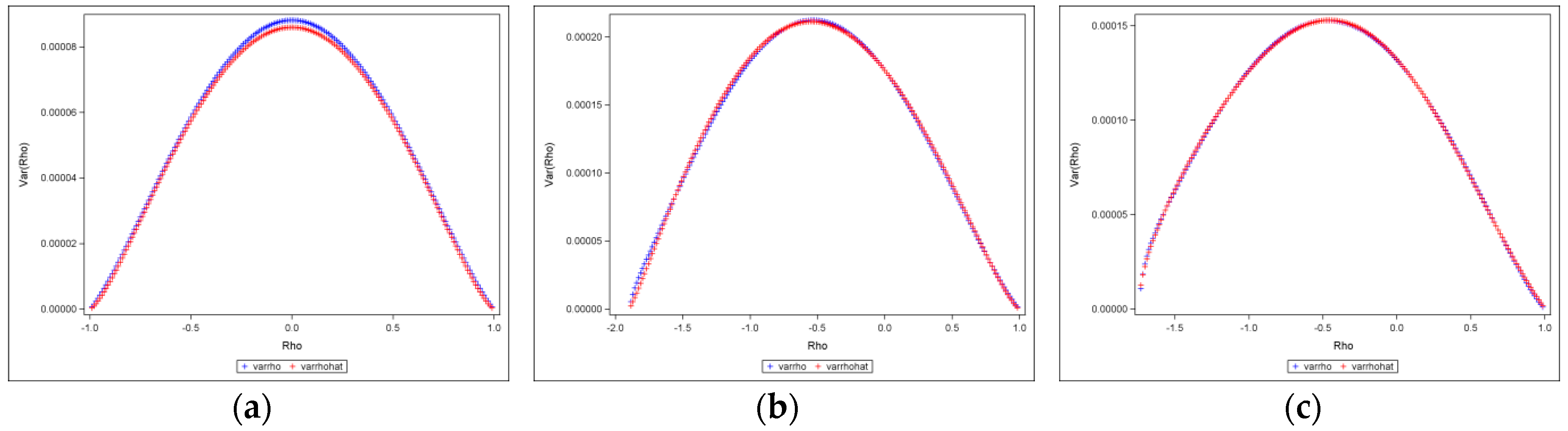
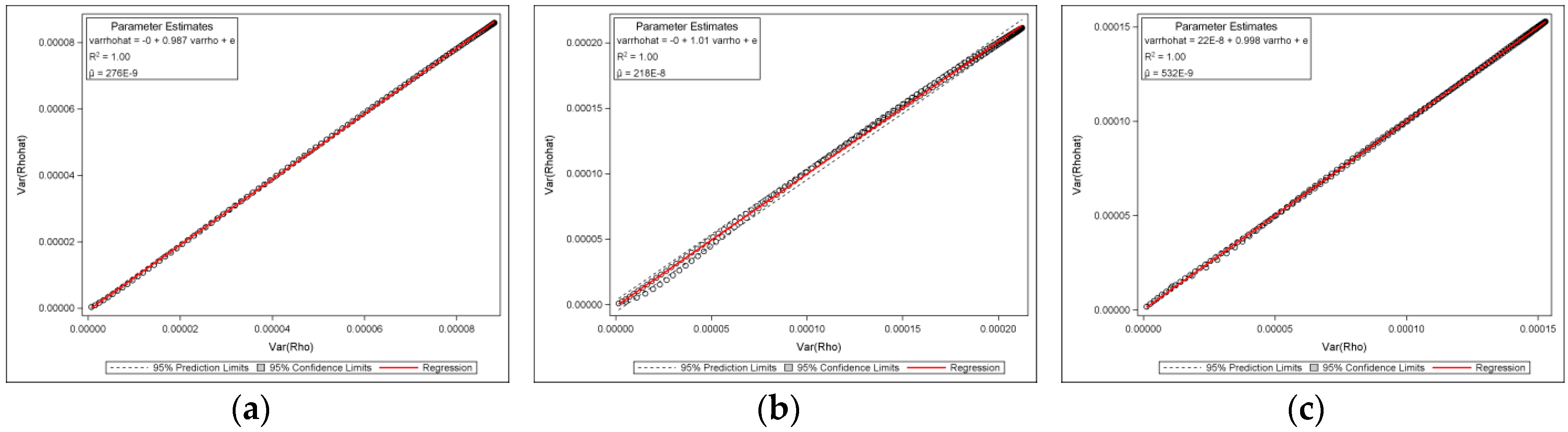
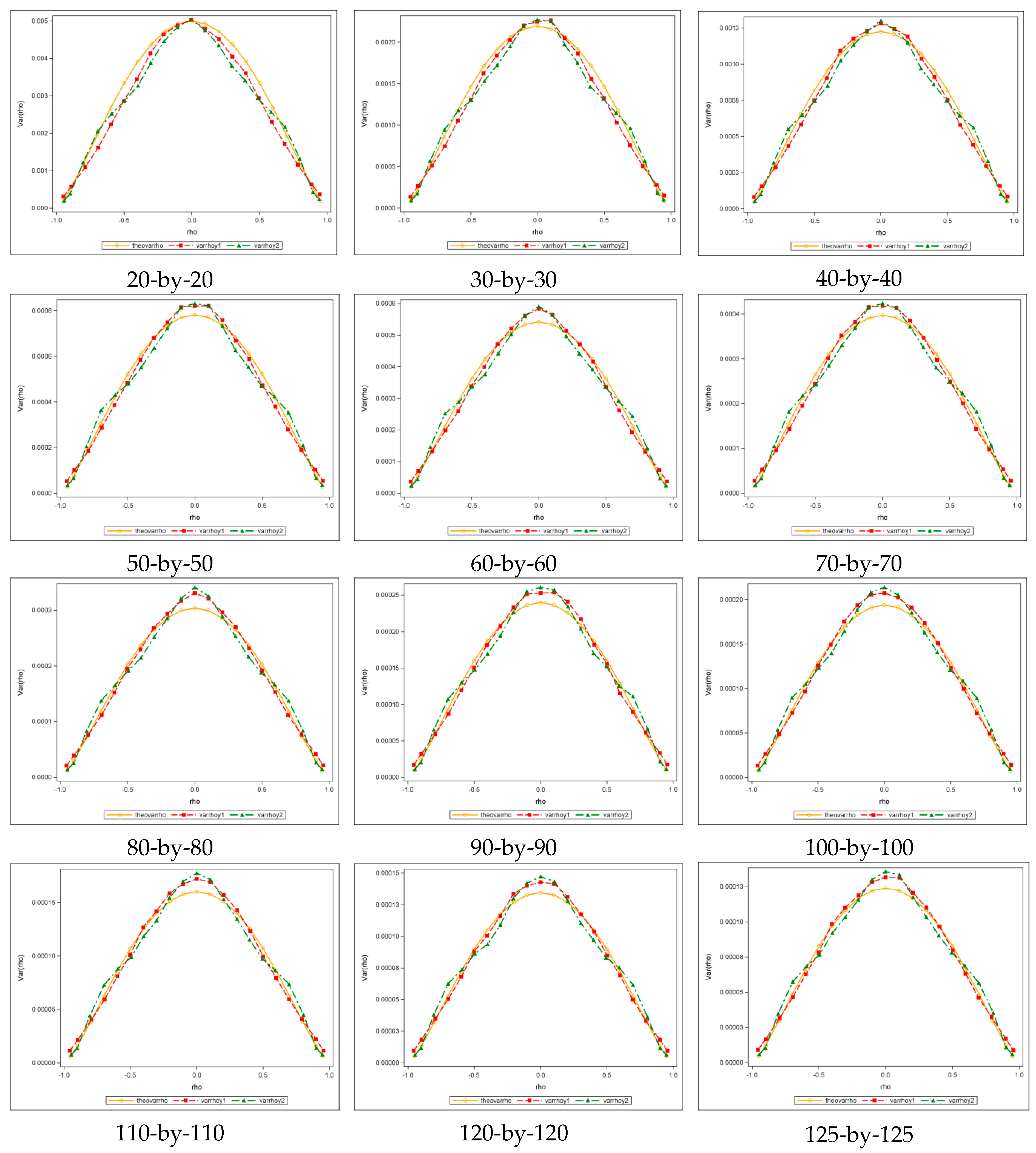
Figure 4 shows selected results of 150-by-150 ($n=22,500$) lattices for the square rook, square queen, and hexagonal cases. It presents theoretical plots (red) superimposed on the original scatter plots (blue), showing that the sampling variance of $\widehat{\rho }$ is Beta-distributed with equal shape and scale parameters, and that the theoretical and the original plots closely correspond, which is also corroborated by the bivariate regression plots and their accompanying $R^2$ values of nearly 1 (see Appendix A Figure A2).

To evaluate the validity of the theoretical equations listed in Table 3, simulation experiments were conducted.

3.2.3. Simulation Experiments

For each of the three cases, 24 groups of experiments of different sample sizes (from 10-by-10 to 125-by-125) were done, and for each sample size, combinations of two treatments (i.e., employing an approximated Jacobian term [36,37] and employing [35] a new algorithm for MLEs) were applied for the pure SAR model. For a square rook case, $\rho$ took 21 values (from −0.9 to 0.9 with a 0.1 increment, and ±0.95) within its feasible range $\left(-1,1\right)$, and 10,000 replications were executed per value per method. 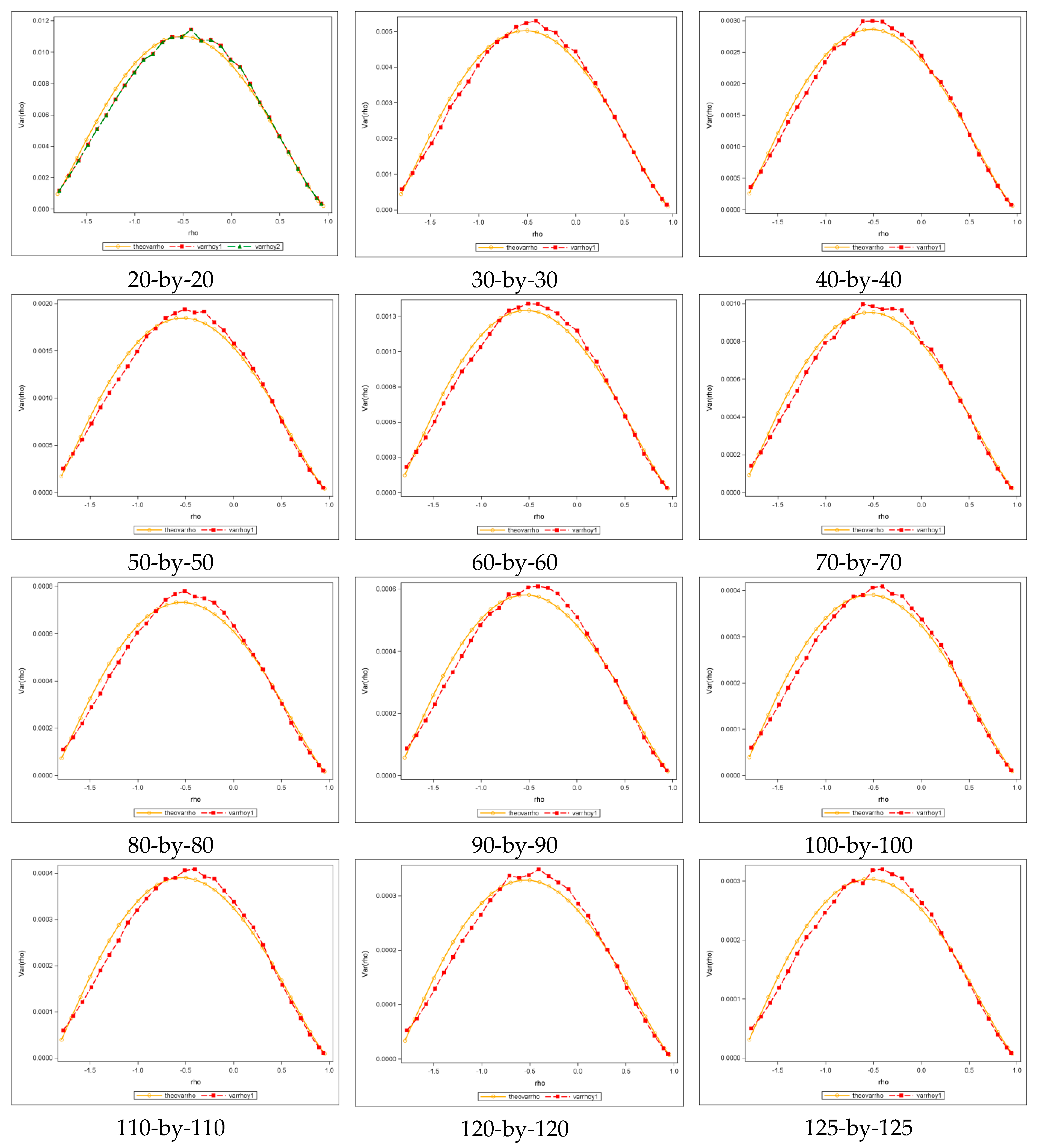For a square queen case, $\rho$ took 29 values (from −1.8 to 0.9 with a 0.1 increment, and 0.95) within its feasible range $\left(-1.9,1\right)$, and 10,000 replications were executed per value per method. 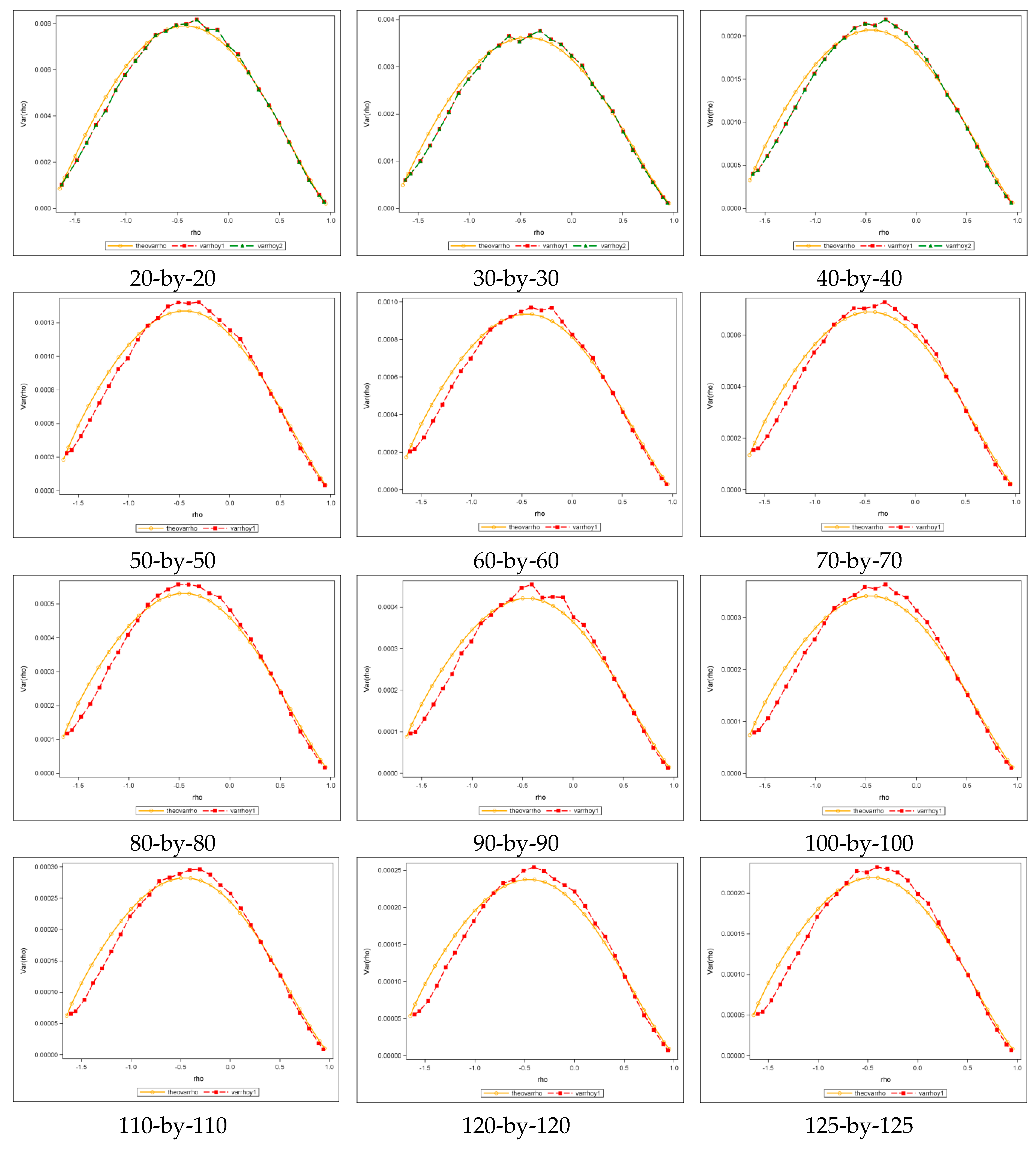For a hexagonal case, $\rho$ took 28 values (from −1.6 to 0.9 with a 0.1 increment, and −1.65, 0.95) within its feasible range $\left(-1.74,1\right)$, and 10,000 replications were executed per value per method.

Table 4. Methods employed with a 10-by-10 lattice *.

Treatment	ExactJacob	AppJacob1	AppJacob2	AppJacob3
Original MLEs	SR, SQ, H	-	-	SQ, H
Griffith’s MLEs (2015)	-	SR	SR	SQ, H

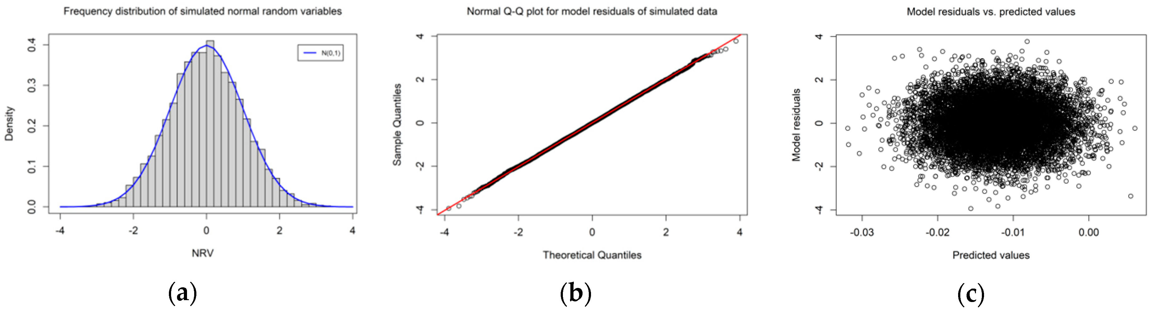
* SR, SQ, and H represent square rook, square queen, and hexagonal cases, respectively. AppJacob1 and AppJacob2 refer to approximated Jacobian Equations (10) and (11) in [35]. AppJacob3 is Equation (8).

shows different treatment combinations that were employed by the three cases with sample size 100 (i.e., 10-by-10 lattice). Full information about the simulations appears in Appendix C (

Table A2. Simulation experiments employing $\rho$ within its feasible range.

Regular Square Rook			Regular Square Queen			Regular Hexagonal Tessellation
Sample Size	Number of Methods	Number of Replications	Sample Size	Number of Methods	Number of Replications	Sample Size	Number of Methods	Number of Replications
10-by-10	3	3*21*10,000	10-by-10	3	3*29*10,000	10-by-10	3	3*28*10,000
15-by-15	2	2*21*10,000	15-by-15	2	2*29*10,000	15-by-15	2	2*28*10,000
20-by-20	2	2*21*10,000	20-by-20	2	2*29*10,000	20-by-20	2	2*28*10,000
25-by-25	2	2*21*10,000	25-by-25	1	29*10,000	25-by-25	2	2*28*10,000
30-by-30	2	2*21*10,000	30-by-30	1	29*10,000	30-by-30	2	2*28*10,000
35-by-35	2	2*21*10,000	35-by-35	1	29*10,000	35-by-35	2	2*28*10,000
40-by-40	2	2*21*10,000	40-by-40	1	29*10,000	40-by-40	2	2*28*10,000
45-by-45	2	2*21*10,000	45-by-45	1	29*10,000	45-by-45	1	28*10,000
50-by-50	2	2*21*10,000	50-by-50	1	29*10,000	50-by-50	1	28*10,000
55-by-55	2	2*21*10,000	55-by-55	1	29*10,000	55-by-55	1	28*10,000
60-by-60	2	2*21*10,000	60-by-60	1	29*10,000	60-by-60	1	28*10,000
65-by-65	2	2*21*10,000	65-by-65	1	29*10,000	65-by-65	1	28*10,000
70-by-70	2	2*21*10,000	70-by-70	1	29*10,000	70-by-70	1	28*10,000
75-by-75	2	2*21*10,000	75-by-75	1	29*10,000	75-by-75	1	28*10,000
80-by-80	2	2*21*10,000	80-by-80	1	29*10,000	80-by-80	1	28*10,000
85-by-85	2	2*21*10,000	85-by-85	1	29*10,000	85-by-85	1	28*10,000
90-by-90	2	2*21*10,000	90-by-90	1	29*10,000	90-by-90	1	28*10,000
95-by-95	2	2*21*10,000	95-by-95	1	29*10,000	95-by-95	1	28*10,000
100-by-100	2	2*21*10,000	100-by-100	1	29*10,000	100-by-100	1	28*10,000
105-by-105	2	2*21*10,000	105-by-105	1	29*10,000	105-by-105	1	28*10,000
110-by-110	2	2*21*10,000	110-by-110	1	29*10,000	110-by-110	1	28*10,000
115-by-115	2	2*21*10,000	115-by-115	1	29*10,000	115-by-115	1	28*10,000
120-by-120	2	2*21*10,000	120-by-120	1	29*10,000	120-by-120	1	28*10,000
125-by-125	2	2*21*10,000	125-by-125	1	29*10,000	125-by-125	1	28*10,000

). For a specific $\rho$, 10,000 simulated values were generated whose frequency distribution was approximately normal, and from which its mean and variance were extracted.

These experiments contend with two complications: approximating the Jacobian term, and clarifying its derivation for the nonlinear regression model in SAS. For the square rook adjacency case, two forms of approximation furnished by [36] were employed. For the square queen and hexagon adjacency cases, the following approximation [37] was used:

$$\begin{gathered} \mathit{J}\mathit{a}\mathit{c}={\alpha }_1\ast \left[\frac{ln\left(1-\rho \ast {\lambda }_{min}\right)}{\rho \ast {\lambda }_{min}}+1-{\delta }_1\ast \ln \left(1-\rho \ast {\lambda }_{min}\right)\right]+{\alpha }_2 \\ \ast \left[\frac{ln\left(1-\rho \ast {\lambda }_{max}\right)}{\rho \ast {\lambda }_{max}}+1-{\delta }_2\ast \ln \left(1-\rho \ast {\lambda }_{max}\right)\right], \end{gathered}$$

(8)

where $\mathit{J}\mathit{a}\mathit{c}$ denotes an approximated Jacobian term. The default derivative of the Jacobian term employed in SAS is misleading. Its correct form, Equation (A2), is presented in Appendix D. Griffith [35] (p. 2149) furnishes a new algorithm to avoid the massive matrix calculation in the MLEs, which effectively reduces the execution time. This algorithm is employed in this paper.

Figure 5 includes 10-by-10 results for the regular square rook, regular square queen, and regular hexagonal tessellation cases. In all these figures, the theoretical values are presented by smooth orange curves. Selected sampling distributions of weak, moderate, and strong positive $\rho$ for a 10-by-10 lattice are presented in Appendix E to illustrate the asymptotic normality of its sampling distribution.

Figure 5a portrays variance values for a systematic sample of 21 points (from −0.95 to 0.95) and a square rook case. Not including the orange graph, there are three other colored graphs in Figure 5a, where the blue stands for the exact values, and the red and green represent two different approximated calculations. The exact and approximated values are close, while a small gap appears between the blue-red-green and the orange graphs around the peak. The gap almost disappears when the sample size becomes 400 (20-by-20, see Appendix FFigure A4), and then appears again, but has no big change as the sample size increases. The gap is the difference between the theoretical and the exact values, and depicts the accuracy of the theoretical formulae—a smaller gap indicates a better approximation. Figure 5b portrays variance values for a systematic sample of 29 points (from −1.8 to 0.95) and a square tessellation with a queen adjacency case. To obtain the two results, one (the red) was calculated by approximating the Jacobian term and using a simplified algorithm for ML estimation [35], whereas the other (the green) was calculated by approximating the Jacobian term and using the conventional ML estimation implementation. Results calculated by these two methods are coincident, and they are not only considerably close to the exact graph (the blue in Figure 5b), but also close to the theoretical curves; the variance plots for larger sample sizes are shown in Appendix F (Figure A5), in which the theoretical (orange) and one approximation (red) are portrayed (except for the 20-by-20 case) because executing the nonlinear regression without the simplified algorithm is extremely time-consuming, and the gaps between the orange and the red are negligible. Figure 5c portrays variance values for a systematic sample of 28 points (from −1.65 to 0.95) computed for the hexagonal case. Here, the two approximations almost perfectly match the exact and theoretical values; variance plots for larger sample sizes appear in Appendix F (Figure A6); the exact variances would be slightly bigger around the maximum values than the theoretical ones when sample size exceeds 1600 (40-by-40), whereas values along the two sides match reasonably well.

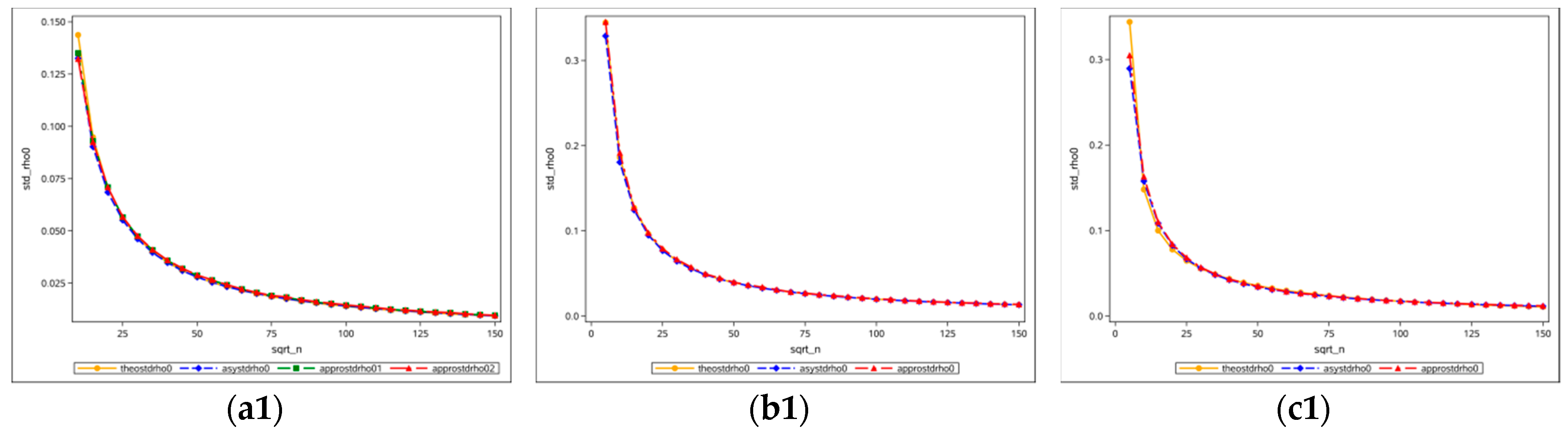
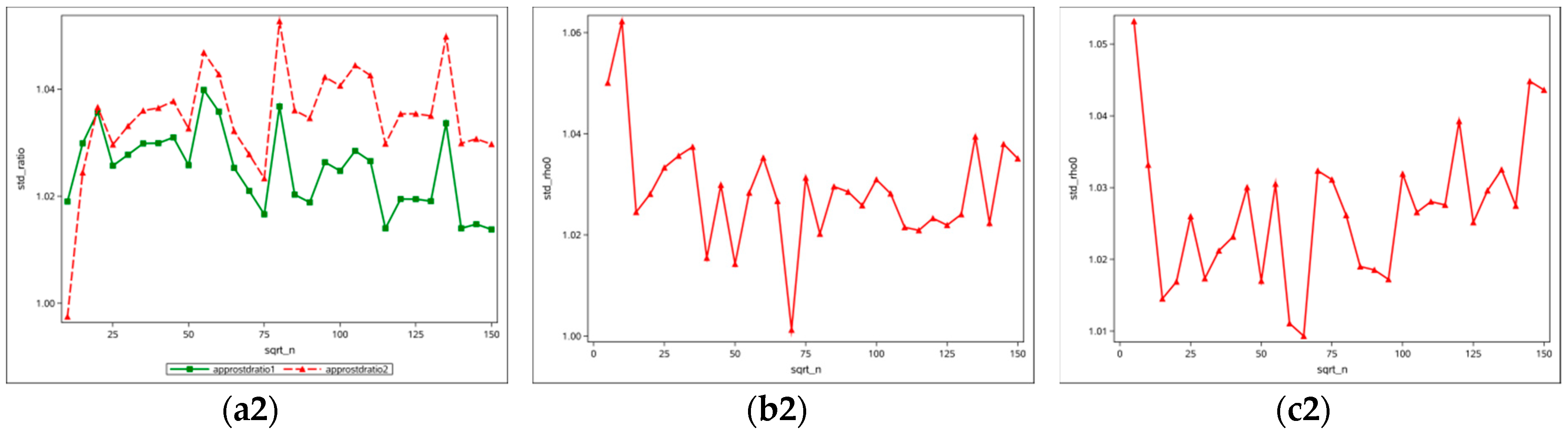
Figure 6 presents convergence plots of variances at $\rho =0$. The top row presents convergence curves whose horizontal axis is the square root of the sample size (from 5 to 150), and whose vertical axis is the standard deviation. Different colors indicate different calculation methods; for example, the orange denotes the theoretical calculated variance of $\rho$ at zero, the blue denotes the asymptotic (formulae in Table 2) computed variance, the green and red respectively denote variance calculated with simulation experiments using the two methods approximating the Jacobian term (two methods exist for the square rook adjacency, whereas only one for the square queen and hexagonal adjacencies). The bottom row shows the standard-deviation-to-square-root-of-sample-size ratio (from 5 to 150); the green and red lines denote those standard deviations calculated with simulation experiments versus the asymptotically calculated standard deviations. Figure 6(a1,a2) are from the results of a square rook case, Figure 6(b1,b2) display the results from a square queen case, and Figure 6(c1,c2) portray the results from a hexagonal case. All of the trajectory curves appear to converge to zero, and all standard deviation ratios fluctuate around 1, when sample size goes to infinity.

4. A Simulated Zero Spatial Autocorrelation Scenario, and Two Nonzero Empirical Examples

Section 3 furnishes the sampling distribution of the nonzero SA parameter of the pure SAR model; one possible application of this contribution is to conduct hypothesis testing for a nonzero $\rho$. Thus, the next section includes two empirical examples that represent moderate and strong positive SA, and to illustrate a zero SA case (rarely encountered in empirical data), simulated data were generated as well. Considering the normality of its sampling distribution, a Z test of the form $\left(\rho -{\rho }_0\right)/sd\left(\rho \right)$ can be used to evaluate the estimated $\rho$ value. Let the significance level $\alpha$ be 0.05, and for a two-sided hypothesis test as employed in this paper, the critical values would be ±1.96 (i.e., any value less than −1.96, or bigger than 1.96 leads to a rejection of the null hypothesis).

4.1. A Description of the Selected Datasets

For the zero SA case, a 100-by-100 ($n=10,000$) landscape (Goslee [48] furnishes R code for generating square lattices) with 10,000 numbers conforming to $N\left(0,1\right)$ randomly assigned on it was generated. Figure 7a illustrates this landscape, with colors ranging from red to green portraying values of different levels. For the moderate SA case, a census dataset with 184 subdistricts for Wuhan, China (2010) (The statistical data come from the “Tabulation on the 2010 population census of China”, http://www.stats.gov.cn/tjsj/pcsj/rkpc/6rp/indexch.htm, and the blocks map comes from the Wuhan Land Resources and Planning Bureau) was employed. The target variable was set to be the percentage of 0-to19-year-old individuals in the population (denoted as 0–19%). Figure 7b illustrates the geographic distribution of 0–19% (ranging from 7.83 to 39.74) across Wuhan administrative districts, with the green representing areas of low rates and the red representing areas of high rates. Relatively low 0–19% areas cluster in the central urban sections, while relatively high 0–19% areas cluster in suburban regions. Because of the irregularity of its configuration, new simulation experiments were conducted to obtain the sampling variance of the SA parameter. Detailed information can be found in Appendix G. For the strong SA case, a Landsat 7 Enhanced Thematic Mapper Plus (ETM+) remotely sensed image downloaded from the USGS EarthExplore (https://earthexplorer.usgs.gov/) was employed. This image is of the Yellow Mountain region of China on 8 October 2002. Its original form is 7811-by-7051 ($n=55,075,361$) pixels, and it includes spectral bands B1-B8, with B1-B7 at a spatial resolution of 30 meters, and B8 having a spatial resolution of 15 meters. In order to be consistent with the magnitude of the other cases, a 100-by-100 patch, which displays the topographic landscape with green areas representing lower elevation and buff-to-white strips depicting mountain ridges with bare rocks, was cropped from the original image, and constitutes the study area across which the normalized difference vegetation index (NDVI) was calculated. The adjacency scheme employed to identify neighbors for all three cases was the rook (i.e., edge connections only), because for the irregular configuration (Figure 7b), the rook and queen (i.e., edge and point connections) would render very close results as adjacent administrative districts always have common boundaries; and for the two square cases (Figure 7a,c), although numerical results would be different, the adjacency definition has little impact on the conclusion.

In the case of moderate positive SA, the response variable 0–19% (YR, as denoted in

Table 5. Results of zero, moderate, and strong positive spatial autocorrelation (SA) examples.

Dataset	Random Landscape	Wuhan Census Blocks	Yellow Mountain Image
Response variable	Pseudo-random numbers	$3.67-11.79\ast {\mathit{e}}^{-6.59\ast YR}$	$1.46\ast {\mathit{e}}^{4.78\ast NDVI}-2.70$
Null hypothesis ($H_0$)	${\rho }_0=0$	${\rho }_0=0.7$	${\rho }_0=0.95$
MC	0.0051	0.5304	0.9077
$\widehat{\rho }$	0.0101	0.7080	0.9697
$sd\left(\widehat{\rho }\right)$	0.0139	0.0598	0.0019
z-score	0.7254	0.1338	10.1762
p-value	0.4682	0.8935	<2.5314e-24
*95% CI of $\widehat{\rho }$	[−0.0171, 0.0373]	[0.5908, 0.8252]	[0.9659, 0.9735]
Conclusion	Failed to reject $H_0$	Failed to reject $H_0$	Reject $H_0$

*95% confidence intervals of model estimated $\rho$ are calculated to determine the range in which the ${\rho }_0$ will not be rejected.

) was subjected to an exponential transformation to make it better align with a bell-shaped curve, hence satisfying an assumption of the pure SAR model; the Shapiro-Wilk test statistic for the original 0–19% was 0.91, increasing to 0.99 after this transformation. For the strong positive SA case, an exponential transformation was also applied to NDVI to achieve better symmetry; considering its large sample size, the Kolmogorov-Smirnov (KS) normality test was employed, and the transformation decreased the KS statistic from 0.4250 to 0.0238. Thus, the transformed 0–19% and NDVI constituted the response variables of those SAR models for which the moderate and strong levels of SA parameters $\rho$ were estimated, respectively. Data transformation and normality testing details for model residuals are presented in Appendix H, and scatter plots of residual-predicted values for assessing the homoscedasticity of model residuals, and thus the validity of the regression model, are also included.

4.2. Results and Explanations

Results are summarized in Table 5, which also includes the MC values.

There are two indexes appearing in this table to indicate the level of SA: the MC, and the SAR model estimated $\rho$ (i.e., $\widehat{\rho }$), both of which represent the same level (i.e., nearly zero, moderate, and strong) of SA, but with different values; the MC is directly calculated with the observations, and $\widehat{\rho }$ is the ML estimate for the pure SAR model in which the neighborhood was defined by rook adjacency. For the random case, the MC value is 0.0051, which indicates nearly zero SA, while $\widehat{\rho }$ is 0.0101; the z-score and p-value indicate a failure to reject the null hypothesis of ${\rho }_0=0$, which verifies that those pseudo-random numbers conforming to $N\left(0,1\right)$ were randomly distributed on the 100-by-100 lattice. For the Wuhan census blocks case, the MC value of 0.53 indicates moderate SA, while $\widehat{\rho }=0.7080$ corresponds to a first-order spatial correlation of roughly 0.45 (e.g., [29] (§2.2.1); [45] (p. 33)). Accordingly, a failure to reject the null hypothesis ${\rho }_0=0.7$ for moderate SA is understandable. In the case of the Yellow Mountain remotely-sensed image, the MC value of 0.9077 indicates a high level of SA, and $\widehat{\rho }=0.9697$ corresponds to a first-order spatial correlation of roughly 0.90. For this strong SA case, setting the null hypothesis of ${\rho }_0=0.95$ is still rejected. Reasons for the rejection may include: (1) when referring to the logistic curve in Figure 3a, those $\rho$ values that indicate strong positive SA may be restricted to a very narrow interval, say $\left(0.95, 1\right)$, while ${\rho }_0=0.95$ corresponds to a moderate MC value (around 0.5); and, (2) the variance of $\widehat{\rho }$ approaches 0 when the sample size becomes large and $\rho$ approaches 1, and the nearly zero variance leads to a high z-score and a narrow confidence interval, and thus an extremely significant p-value.

5. Conclusions and Discussion

The main contribution of this paper is furnishing the sampling distribution of the nonzero SA parameter of the SAR model, which is frequently employed in a wide range of disciplines whose study observations are connected with geographical attributes or locations. More specifically, the sampling distribution was constructed for three specific spatial structures (i.e., regular square rook and queen, and hexagonal tessellations); the former two are usually used for remotely sensed images (raster data), while the latter is preferred for spatial sampling designs and aggregations. As shown with graphics and functions, the curve shape of the parameter $\rho$ against the MC is sigmoid, which indicates that the MC should better differentiate SA levels and is more coincident with intuition (e.g., a MC value of 0.5 quantifies moderate SA, whereas the $\rho$ value for the same level may be larger than 0.7, which conjures up a vision of moderate-to-strong SA at first glance). This may suggest that the MC could be better for assessing the level of SA. In addition, the sampling variance of the parameter seems to conform to a beta distribution with equal scale and shape parameters (larger than 1). A difference in these distributions between the square rook and the other two is that the parabola-shaped curve is symmetric at zero for the square rook adjacency, whereas the symmetry is at negative points for the square queen and hexagonal adjacencies.

One merit of this contribution is that it implements hypothesis testing for a nonzero null hypothesis. For illustrative purposes, two empirical examples for moderate and strong SA were selected, as was a zero null hypothesis case employing simulated data exhibiting a random map pattern. For this random case, the result indicates a failure to reject the null hypothesis, which is in accordance with our expectation. For the moderate case, prior knowledge that $\rho$ and the MC have a logistic relationship (i.e., MC values beyond, e.g., (−0.3, 0.3) correspond to extreme $\rho$ values) results in positing a null hypothesis of ${\rho }_0=0.7$; thus, the null hypothesis is not rejected. For the strong SA case, the null hypothesis of ${\rho }_0=0.95$ is rejected mainly because of the large sample size (i.e., $n=10,000$) and the closeness between 0.95 and 1, both of which result in an extremely small variance. 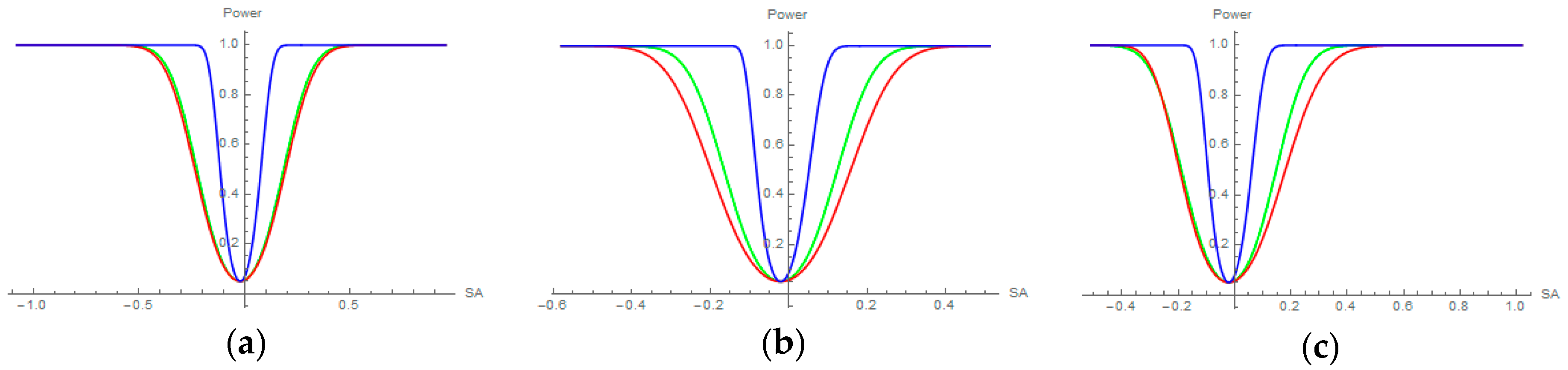These examples verify that the uncovered sampling distribution results are credible (the standard error for ${\rho }_0=0$ is 0.0141, corresponding to a z-score of 0.7188, which has a very small difference of 0.0066 with the z-score 0.7254 appearing in Table 5). In addition, a by-product of this contribution is the visualization of statistical power curves for SA statistics [42]. Because the SA parameter can be expressed in terms of the MC, their power curves can be plotted with a common measurement scale (see Appendix I).

Future work needs to refine, and hopefully simplify, the variance expression for the hexagonal case; one way to achieve this end is to increase the number of experiments (the current variance-$\rho$ function is based upon 14 groups of datasets (i.e., 7-by-7 to 70-by-70) to estimate its parameters). Extensions can be made for more complicated landscapes, such as a combination of hexagons and pentagons, partitionings with distorted hexagons (i.e., ISEA3H as a hexagonal Discrete Global Grid System; [43]); these may be described with appropriate spatial weights matrices, where for the former, expressions like those listed in Table 2 need to be derived, and for the latter, a spatial weights matrix containing metrics based upon side length or hexagon area may be more reasonable than a binary version. An important issue illustrated by the last example meriting emphasis is that the formal hypothesis testing or its p-value may no longer make sense because of the large-to-massive sample size involved. For example, the “confidence interval” of 0.9697 is [0.9659, 0.9735], in which the null hypothesis value should be contained; otherwise, the null hypothesis is rejected. A cause of this “always significant” phenomenon is the extremely small variance for a very big sample size, which creates the necessity to develop a new criterion to substitute for statistical significance when analyzing spatial data with large-to-massive sample sizes. This is a meaningful research theme that needs attention in the future.

References

1. Li, H.; Calder, C.A.; Cressie, N. Beyond Moran’s I: Testing for Spatial Dependence Based on the Spatial Autoregressive Model. Geogr. Anal. 2007, 39, 357–375. [Google Scholar] [CrossRef]
2. Robinson, P.M.; Rossi, F. Refined tests for spatial correlation. Econom. Theory 2015, 31, 1249–1280. [Google Scholar] [CrossRef]
3. López, F.; Matilla-García, M.; Mur, J.; Marín, M.R. A non-parametric spatial independence test using symbolic entropy. Reg. Sci. Urban Econ. 2010, 40, 106–115. [Google Scholar] [CrossRef] [Green Version]
4. Gotelli, N.J.; Ulrich, W. Statistical challenges in null model analysis. Oikos 2012, 121, 171–180. [Google Scholar] [CrossRef]
5. Griffith, D.A. Spatial statistics: A quantitative geographer’s perspective. Spat. Stat. 2012, 1, 3–15. [Google Scholar] [CrossRef]
6. Bivand, R. Package ‘spdep’. Available online: https://cran.r-project.org/web/packages/spdep/spdep.pdf (accessed on 24 October 2018).
7. Hong, Y.; White, H. Asymptotic Distribution Theory for Nonparametric Entropy Measures of Serial Dependence. Econometrica 2005, 73, 837–901. [Google Scholar] [CrossRef] [Green Version]
8. Matilla-García, M.; Marín, M.R. A non-parametric independence test using permutation entropy. J. Econom. 2008, 144, 139–155. [Google Scholar] [CrossRef] [Green Version]
9. Montgomery, D.C.; Peck, E.A.; Vining, G.G. Introduction to Linear Regression Analysis; Wiley: Hoboken, NJ, USA, 2012. [Google Scholar]
10. Burt, J.E.; Barber, G.M.; Rigby, D.L. Elementary Statistics for Geographers; Guilford Publications: New York, NY, USA, 2009. [Google Scholar]
11. Bewick, V.; Cheek, L.; Ball, J. Statistics review 7: Correlation and regression. Crit. Care 2003, 7, 451–459. [Google Scholar] [CrossRef]
12. Provost, B.S. Closed-Form Representations of the Density Function and Integer Moments of the Sample Correlation Coefficient. Axioms 2015, 4, 268–274. [Google Scholar] [CrossRef]
13. Ames, E.; Reiter, S. Distributions of Correlation Coefficients in Economic Time Series. J. Am. Stat. Assoc. 1961, 56, 637–656. [Google Scholar] [CrossRef]
14. Lee, M.Y. The Effect of Nonzero Autocorrelation Coefficients on the Distributions of Durbin-Watson Test Estimator: Three Autoregressive Models. Expert J. Econ. 2014, 2, 85–99. [Google Scholar]
15. Mead, R. A Mathematical Model for the Estimation of Inter-Plant Competition. Biometrics 1967, 23, 189–205. [Google Scholar] [CrossRef] [PubMed]
16. Moran, P.A.P. Notes on Continuous Stochastic Phenomena. Biometrika 1950, 37, 17–23. [Google Scholar] [CrossRef] [PubMed]
17. Lesage, J.; Kelly Pace, R. Introduction to Spatial Econometrics; CRC Press: Boca Raton, FL, USA, 2009; Volume 1. [Google Scholar]
18. Cliff, A.D.; Ord, J.K. Spatial Processes: Models & Applications; Pion: London, UK, 1981. [Google Scholar]
19. Griffith, D.A.; Layne, L.J. A Casebook for Spatial Statistical Data Analysis: A Compilation of Analyses of Different Thematic Data Sets; Oxford University Press: Oxford, UK, 1999. [Google Scholar]
20. Ver Hoef, J.M.; Hanks, E.M.; Hooten, M.B. On the relationship between conditional (CAR) and simultaneous (SAR) autoregressive models. Spat. Stat. 2018, 25, 68–85. [Google Scholar] [CrossRef] [Green Version]
21. Cliff, A.D.; Ord, J.K. Spatial Autocorrelation; Pion Limited: London, UK, 1973. [Google Scholar]
22. Sokal, R.R.; Oden, N.L. Spatial autocorrelation in biology: 1. Methodology. Biol. J. Linn. Soc. 1978, 10, 199–228. [Google Scholar] [CrossRef] [Green Version]
23. Sokal, R.R.; Oden, N.L. Spatial autocorrelation in biology: 2. Some biological implications and four applications of evolutionary and ecological interest. Biol. J. Linn. Soc. 1978, 10, 229–249. [Google Scholar] [CrossRef] [Green Version]
24. Legendre, P. Spatial Autocorrelation: Trouble or New Paradigm? Ecology 1993, 74, 1659–1673. [Google Scholar] [CrossRef] [Green Version]
25. Auchincloss, A.H.; Gebreab, S.Y.; Mair, C.; Diez Roux, A.V. A Review of Spatial Methods in Epidemiology, 2000–2010. Annu. Rev. Public Health 2012, 33, 107–122. [Google Scholar] [CrossRef] [Green Version]
26. Anselin, L.; Florax, R.; Rey, S.J. Advances in Spatial Econometrics: Methodology, Tools and Applications; Springer: Berlin/Heidelberg, Germany, 2004. [Google Scholar]
27. Mustafa, A.; Van Rompaey, A.; Cools, M.; Saadi, I.; Teller, J. Addressing the determinants of built-up expansion and densification processes at the regional scale. Urban Stud. 2018, 55, 3279–3298. [Google Scholar] [CrossRef] [Green Version]
28. Goodchild, M.F. Geographical information science. Int. J. Geogr. Inf. Syst. 1992, 6, 31–45. [Google Scholar] [CrossRef]
29. Bartlett, M.S. The Statistical Analysis of Spatial Pattern; Chapman and Hall: Boca Raton, FL, USA, 1975. [Google Scholar]
30. Whittle, P. On stationary processes in the plane. Biometrika 1954, 41, 434–449. [Google Scholar] [CrossRef]
31. Ord, K. Estimation Methods for Models of Spatial Interaction. J. Am. Stat. Assoc. 1975, 70, 120–126. [Google Scholar] [CrossRef]
32. Cressie, N.A.C. Statistics for Spatial Data; Wiley: Hoboken, NJ, USA, 1993. [Google Scholar]
33. Griffith, D.A. Estimating Spatial Autoregressive Model Parameters with Commercial Statistical Packages. Geogr. Anal. 1988, 20, 176–186. [Google Scholar] [CrossRef]
34. Griffith, D.A. Simplifying the normalizing factor in spatial autoregressions for irregular lattices. Pap. Reg. Sci. 1992, 71, 71–86. [Google Scholar] [CrossRef]
35. Griffith, D.A. Approximation of Gaussian spatial autoregressive models for massive regular square tessellation data. Int. J. Geogr. Inf. Sci. 2015, 29, 2143–2173. [Google Scholar] [CrossRef]
36. Griffith, D.A. Faster maximum likelihood estimation of very large spatial autoregressive models: an extension of the Smirnov–Anselin result. J. Stat. Comput. Simul. 2004, 74, 855–866. [Google Scholar] [CrossRef]
37. Griffith, D.A. Extreme eigenfunctions of adjacency matrices for planar graphs employed in spatial analyses. Linear Algebra Its Appl. 2004, 388, 201–219. [Google Scholar] [CrossRef]
38. Griffith, D.A. Eigenfunction properties and approximations of selected incidence matrices employed in spatial analyses. Linear Algebra Its Appl. 2000, 321, 95–112. [Google Scholar] [CrossRef]
39. Kelejian, H.H.; Prucha, I.R. A Generalized Moments Estimator for the Autoregressive Parameter in a Spatial Model. Int. Econ. Rev. 1999, 40, 509–533. [Google Scholar] [CrossRef] [Green Version]
40. Kelejian, H.H.; Prucha, I.R. Specification and estimation of spatial autoregressive models with autoregressive and heteroskedastic disturbances. J. Econom. 2010, 157, 53–67. [Google Scholar] [CrossRef] [Green Version]
41. Walde, J.; Larch, M.; Tappeiner, G. Performance contest between MLE and GMM for huge spatial autoregressive models. J. Stat. Comput. Simul. 2008, 78, 151–166. [Google Scholar] [CrossRef]
42. Luo, Q.; Griffith, D.A.; Wu, H. The Moran Coefficient and the Geary Ratio: Some Mathematical and Numerical Comparisons. In Advances in Geocomputation; Springer International Publishing: Cham, Switzerland, 2017; pp. 253–269. [Google Scholar]
43. Sahr, K.; White, D.; Kimerling, A.J. Geodesic Discrete Global Grid Systems. Cartogr. Geogr. Inf. Sci. 2003, 30, 121–134. [Google Scholar] [CrossRef]
44. Chun, Y.; Griffith, D.A. Spatial Statistics and Geostatistics: Theory and Applications for Geographic Information Science and Technology; SAGE Publications: Thousand Oaks, CA, USA, 2013. [Google Scholar]
45. Griffith, D.A. Spatial Autocorrelation and Spatial Filtering: Gaining Understanding Through Theory and Scientific Visualization; Springer: Berlin, Germany, 2003. [Google Scholar]
46. Jong, P.; Sprenger, C.; Veen, F. On Extreme Values of Moran’s I and Geary’s c. Geogr. Anal. 1984, 16, 17–24. [Google Scholar] [CrossRef]
47. Griffith, A.D.; Chun, Y. Spatial Autocorrelation and Uncertainty Associated with Remotely-Sensed Data. Remote Sens. 2016, 8, 535. [Google Scholar] [CrossRef]
48. Goslee, S.C. Behavior of Vegetation Sampling Methods in the Presence of Spatial Autocorrelation. Plant Ecol. 2006, 187, 203–212. [Google Scholar] [CrossRef]
1
Ord, 1975, Appendix B, contains a typographical error: a minus should be inserted after the second equality sign of α .
2
There is a typo in [36] (p. 864), the brace needs to be removed.
Figure 1. Selected frequency distributions of simultaneous autoregressive (SAR)-estimated ρ .
Ijgi 07 00476 g001
Figure 2. Three regular surface partitionings: (a) square configuration with rook adjacency; (b) square configuration with queen adjacency; (c) hexagonal configuration.
Ijgi 07 00476 g002
Figure 3. Fitted curves of the MC against ρ for 70-by-70 ( n = 4900 ) surface partitionings: (a) square rook case; (b) square queen case; and, (c) hexagonal case.
Ijgi 07 00476 g003
Figure 4. Fitted curves of the asymptotic variance versus ρ ^ for 150-by-150 ( n = 22 , 500 ) adjacencies: (a) square rook case; (b) square queen case; and, (c) hexagonal case.
Ijgi 07 00476 g004
Figure 5. Variance comparison plots for 10-by-10 ( n = 100 ) tessellations: (a) square rook case; (b) square queen case; (c) hexagonal case.
Ijgi 07 00476 g005
Figure 6. Convergence and variance ratio plots at ρ = 0 . (a1,a2) Square rook variance convergence and ratio plots; (b1,b2) square queen variance convergence and ratio plots; (c1,c2) hexagonal variance convergence and ratio plots.
Ijgi 07 00476 g006aIjgi 07 00476 g006b
Figure 7. Landscapes with different degrees of spatial autocorrelation (SA): (a) a 100-by-100 lattice across which pseudo-random numbers from a standard normal distribution are randomly distributed; (b) 184 census blocks of Wuhan (2010) with 0–19% (ranging from 7.83 to 39.74, with green representing low rates and red representing high rates) displayed; (c) 100-by-100 pixels clipped from the Yellow Mountain region image (2002, with the green representing vegetation and buff-to-white strips depicting mountain ridges).
Ijgi 07 00476 g007