Cartographic Line Generalization Based on Radius of Curvature Analysis


WAT—Military University of Technology, Institute of Geodesy, ul. Gen. Witolda Urbanowicza, 2, 00-908 Warsaw, Poland
*
Authors to whom correspondence should be addressed.
ISPRS Int. J. Geo-Inf. 2018, 7(12), 477; https://0-doi-org.brum.beds.ac.uk/10.3390/ijgi7120477
Submission received: 21 August 2018
/
Revised: 28 November 2018
/
Accepted: 6 December 2018
/
Published: 12 December 2018
(This article belongs to the Special Issue Smart Cartography for Big Data Solutions)
Abstract
:Cartographic generalization is one of the important processes of transforming the content of both analogue and digital maps. The process of reducing details on the map has to be conducted in a planned way in each case when the map scale is to be reduced. As far as digital maps are concerned, numerous algorithms are used for the generalization of vector line elements. They are used if the scale of the map (on screen or printed) is changed, or in the process of smoothing vector lines (e.g., contours). The most popular method of reducing the number of vertices of a vector line is the Douglas-Peucker algorithm. An important feature of most algorithms is the fact that they do not take into account the cartographic properties of the transformed map element. Having analysed the existing methods of generalization, the authors developed a proprietary algorithm that is based on the analysis of the curvature of the vector line and fulfils the condition of objective generalization for elements of digital maps that may be used to transform open and closed vector lines. The paper discusses the operation of this algorithm, along with the graphic presentation of the generalization results for vector lines and the analysis of their accuracy. Treating the set of verification radii of a vector line as a statistical series, the authors propose applying statistical indices of position of these series, connected with the shape of the vector line, as the threshold parameters of generalization. The developed algorithm allows for linking the generalization parameters directly to the scale of the topographic map that was obtained after generalization. The results of the operation of the algorithm were compared to the results of the reduction of vertices with use of the Douglas-Peucker algorithm. The results demonstrated that the proposed algorithm not only reduced the number of vertices, but that it also smoothed the shape of physiographic lines, if applied to them. The authors demonstrated that the errors of smoothing and position of vertices did not exceed the acceptable values for the relevant scales of topographic maps. The developed algorithm allows for adjusting the surface of the generalized areas to their initial value more precisely. The advantage of the developed algorithm consists in the possibility to apply statistical indices that take the shape of lines into account to define the generalization parameters.
1. Introduction
Map content generalization is one of the essential works in processing the information when changing the scale of the map from the larger to the smaller one. Many factors influence the generalization, which depend primarily on the aim of the work and the purpose of the map. These factors affect the type of actions taken to implement the reduction of map content information. These actions can be grouped into four categories of processes, called elements of cartographic generalization [1,2]:
- selection and simplification—defining important data features, preserving and, if possible, highlighting these features, eliminating undesirable details,
- classification—ordering or selection of an appropriate scale for the data and their grouping,
- symbolization—graphic coding of grouped basic features of compared values and their mutual position, and
- induction—application of a logical process of inference in cartography.
Depending on whether the map is being generalized in an analog or digital form, different ways of implementing the main postulates of generalization are possible. Analogue maps, edited and generalized for decades or even hundreds of years in the traditional way, by their very nature are not subject to the processes of computer automation. Otherwise, digital maps, the generalization of which can be computer-aided. The form of their record imposes the necessity of attempting to automate the processes of processing the information that is contained in them [3,4].
2. Related Work
From the point of view of the vector model that is used to present the content of the map and the topology of the objects contained in the content of the maps, can be divided into:
- point e.g., church, town etc.
- lines e.g., borders, roads etc.
- polygons—e.g., land use, sea etc.
Linear elements usually have the form of a vector line on the maps. Most generalization algorithms that are included in the available GIS software are related to the simplification of these elements of map content. The easiest one is the algorithm for removing every nth point (Tobler’s method from 1966) [5]. However, this approach does not take account of the relationship between neighboring points. This method was subject to improvements and it was a contribution to the development of other, more sophisticated ways of generalizing linear elements.
In the 1970s and later, many digital generalization algorithms were developed, most of which refer to relatively simple issues related to one type of elements—with lines [1,6]. The necessary condition for their use is the digital form of the map. The Douglas-Peucker (DP) algorithm [7] is an iterative algorithm that is based on the concepts of the baseline and tolerance zone. The baseline connects the beginning and end points of the generalized line. The first point is called the anchor and the second one is a float. The tolerance zone, the width of which is determined by the user depending on the anticipated degree of generalization, is to ensure the preservation of the character of the most important features of the line. Li and Openshaw [8] presented a new approach to simplifying the course of linear objects that is based on the natural process that people use to observe geographic objects. The method simulates the natural principle that is used by the human eye and brain. The ratio of input and target resolution is used to calculate the so-called “smallest visible object”. The method proved to be effective in detecting and maintaining the general shape of line features. Visvalingam and Whyatt [9] proposed a gradual simplification of linear features using the concept of “effective area”. Based on the analysis and detection of changes in the direction of the line, Wang and Muller [10] proposed a line simplification algorithm.
In recent years, the study of line simplification has focused on shape analysis [11,12], topological consistency assessment [13,14] analysis of geographical characteristics [15,16] and data quality [17,18] Jiang and Nakos [11] presented a new approach to the simplification of lines that is based on the detection of the shape of geographic objects in self-organizing maps. Dyken et al. [13] presented a method of simultaneous simplification of partial curves. This method uses limited Delaunay triangulation to preserve the topological relationships between linear features. Nabil et al. [15] presented a method of line simplification that is based on the Voronoi diagram. It is based on the preliminary division of the complex cartographic curve into a series of simpler fragments. They are then simplified using methods, such as the DP algorithm. With this method you can avoid intersections of input lines. Nöllenburg et al. [16] proposed a method of morphing lines at various levels of detail. The method can be used to continuously generalize linear geographic elements, such as rivers and roads. Stanisławski et al. [17] studied different types of metric assessments, such as Hausdorff distance, segment length, vector shift, surface displacement, and tortuosity for the generalization of linear geographic elements. Their research can provide references to the appropriate settings of the line generalization parameters for the maps at various scales.
Another issue studied in the analysis of the generalization of digital maps was the problem of changing the shape of areal and linear objects whose boundaries were subject to simplification. McMaster [19] presented a method of simplification lines based on the integration of smoothing and simplifying, which is to reduce the change of area. A similar idea is presented by T. Gökgöz et al. [20]. Bose et al. [21] proposed a method to simplify the boundaries of polygons. In their research, according to accepted boundaries of surface changes, the path containing the smallest number of edges was used for simplification. In the study of Buchin et al. [22] is presented the method of area preservation in the process of simplifying polygon boundaries by means of an edge shift operation. In this algorithm, the orientation of polygons is preserved by an edge-shifting operation that is shifted to the inside or outside of the polygons. Another method of analyzing the curvature of vector lines and their generalization is an algorithm that is based on the method of analyzing the course and form of empirical lines. The idea of this generalization method concerning analogue maps was included in Julian Perkal’s works [23,24]. He divided the areas that are distinguished on the map into two types: those that have precisely defined boundaries between them and those whose dividing lines are not clearly defined.
Another known method of generalization is the Chrobak method [25,26], which is based on the so-called elementary triangle. It is a method of simplifying open and closed vector lines depending on the scale and presentation of the map. In this method, the topology of the line that is associated with the hierarchy of three consecutive vertices of vector line is very important, assuming that the initial and final number of vector line vertices are unchanged. In a simplified way, it can be said that these two vertices (two out of three analyzed vertices) form the basis for creating a triangle, and the third vertex determines a point that in the given range maintains the highest height in the triangle while meeting the condition that the sides of this triangle are not smaller than the shortest side of the so-called elementary triangle. The length of the sides of the elementary triangle depends mainly on the scale of the map being developed [27].
3. Algorithm for Checking the Curvature Radius of a Vector Line
Analyzing various approaches to the generalization of linear elements of the topographic digital map, the authors decided to propose a different approach to solve this problem. Due to professional interest in cartography and military topography, we particularly wanted to put emphasis on solving this problem for its application in technological processes of military topographic map production. Maps of this type are performed in two types, both as digital maps that are used in GIS systems and analogue (cartographic) maps used daily in the paper version of the army. Regardless of their scale, they should reflect the character of the terrain elements as faithfully as possible. The proposed algorithm for examining the radius of curvature and the generalization of a vector line described below is based on the method of analyzing the course and shape of empirical lines. The vector line can be defined as a sequence of vectors, where the end of one vector is the beginning of the next. Each two sections have at most one common point. Otherwise, it can be defined as an element of a class of curves defined with the inclusion of an additional condition per function f: (x, y) ≥ ℝ2, mapping the interval in the plane for functions with linear intervals—that is, a function of a real variable whose domain can be broken down into the sum of disjoint compartments in such a way that each function is linear. For the implementation of objective generalization, it was proposed to use the mathematical modeling method of “rolling” the circle on the physical surface of the Earth, just like Perkal proposed [23]. The main factor distinguishing this algorithm is the method of controlling it, based on the analysis of the circle radius value that is described on three consecutive points of a vector line (PS, PC, and PE) open or closed. The points analyzed must meet the basic relationship:
It means that they must belong to a set that fulfills the above condition. This condition determines the belonging of the set of P points to the circle, defined by the Equation (1), where the radius is constant. The radius of this circle, is a measure of the degree of generalization. Due to the way that the algorithm works, it is an iterative algorithm.
If the vector line counts i = 1, …, n points, then the following points are taken for analysis: PS = Pi, PC = Pi+1, PE = Pi+2 from i = 1 to i = n − 2. The starting point of the entire vector line and the end point are invariants and are not subject to the generalization process.
In the case of generalization of an open line, the simplification process starts from the first point of the whole vector line. In the case of a closed line, unless there are other initial conditions, the algorithm selects the point from which the generalization of this line begins. The selection is based on the fact that among all calculated radii of circles based on three consecutive vertices, the vertex with largest radius is selected. The center point (PC) of the three points becomes the starting point of the generalization process.
The generalization process involves the analysis of the ratio of the radius of Rgen generalization radius and the Rver verification radius. The verification radius is the radius of a circle containing three consecutive points of a polyline. The generalization radius Rgen is the radius that is related to the generalized line. Generalization is based on Formula (2), which uses the difference in the length of these radii is checked, and the size of the shortest distance between the chord of the circle based on the first and third point (PS and PE) and the center point (PC):
where: Rgen—radius of the generalization circle; Rver—radius of verification circle; PS—the first point with (starting point) coordinates xS and yS; PC—the focal point coordinates xC and yC; PE—the end point coordinates xE and yE; hdop—permissible Hausdorff distance between the highest point of arc and the chord of the verification circle equal to 0.3 mm * M (M—the denominator of the target map scale, an empirical coefficient related to the accuracy of the topographical map, orthophotomap, and screen vectorization); harc—height of the verification circle arc; d(PS,PE)—chord length.
The application of the fourth case in Formula (2) algorithm is optional and takes place after entering the harc parameter into the procedure.
In order to automate the generalization process and analyze its result, a computer program in Delphi language was written. The analysis of the procedure is shown in Figure 1, Figure 2, Figure 3 and Figure 4.
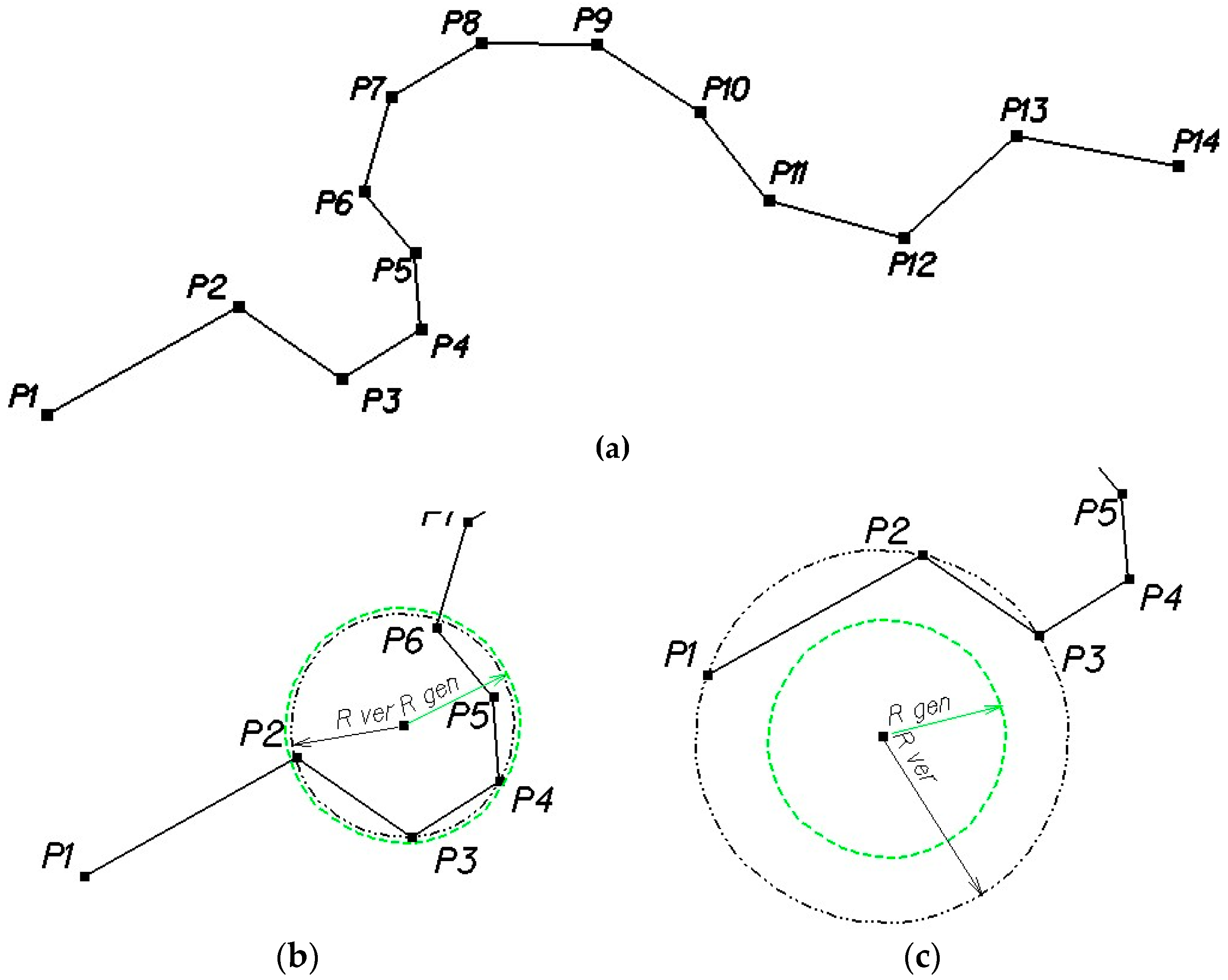
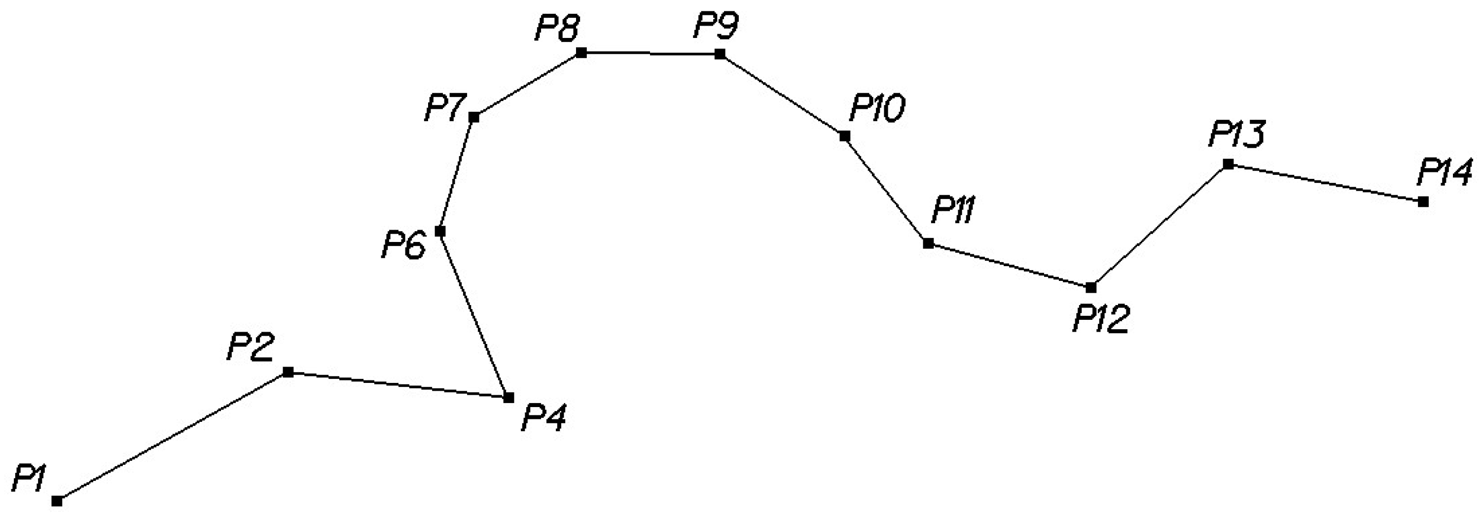
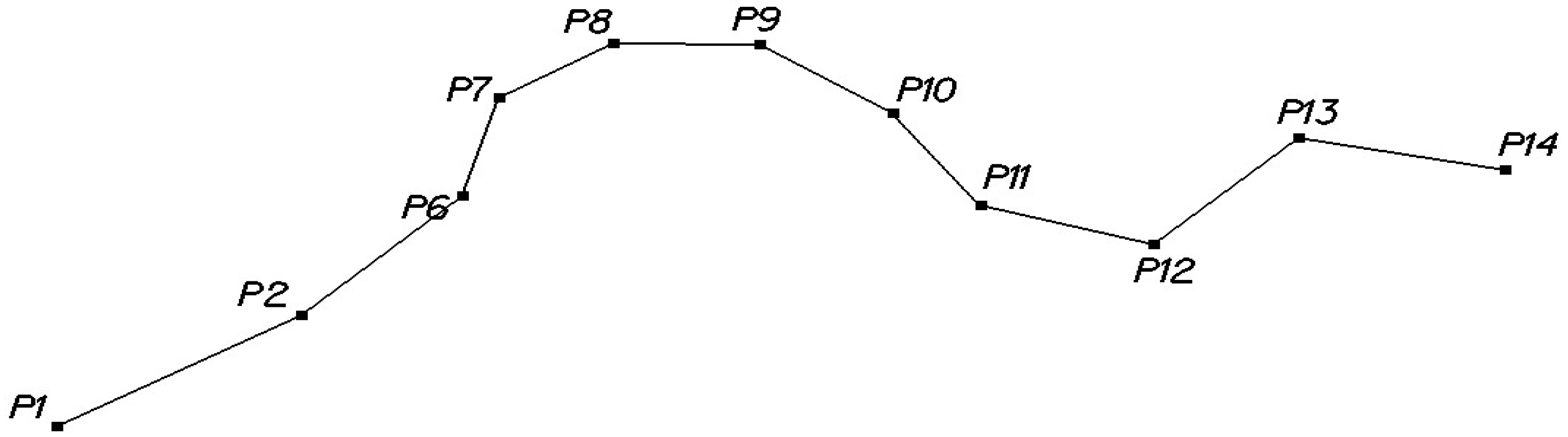
Figure 1a shows the initial vector line subjected to the generalization process. This line contains 14 of the vector line vertices. When generalized, the radius marked Rgen, was taken as the radius limit generalization in the iteration process. The radius of a circle defined by three successive points of a vector line was denoted as Rver (radius of verification). Figure 2 shows the first stage of generalization consisting of:
- determining the actual radius of the circle based on the first three points of the vector line P2 = PS, P3 = PC and P4 = PE;
- checking whether the radius is greater, equal to or smaller than the accepted radius of generalization Rgen and checking whether there is no other vertex of the vector line located inside the circle with a radius equal to the radius of generalization Rgen (the generalization circle);
- depending on the result of the check:
- if the verification radius is smaller than the generalization radius Rver < Rgen (Rwer − Rgen < 0) and the chord length is ds(PS,PE) < 2 × Rgen, then the middle point from the analyzed three vertices is removed from the set of vector line vertices. In the situation shown in Figure 1b, the radius of the circle described on points P2 = PS, P3 = PC, and P4 = PE is shorter than the radius of generalization, so the point P3 = PC will be removed from the set of vector line vertices;
- if the verification radius is greater than or equal to the generic radius Rver ≥ Rgen and ds(PS,PE) > 2 × Rgen, as shown in Figure 1c., then the set of vector line points is left unchanged. The next three vertices are checked, starting from P2;
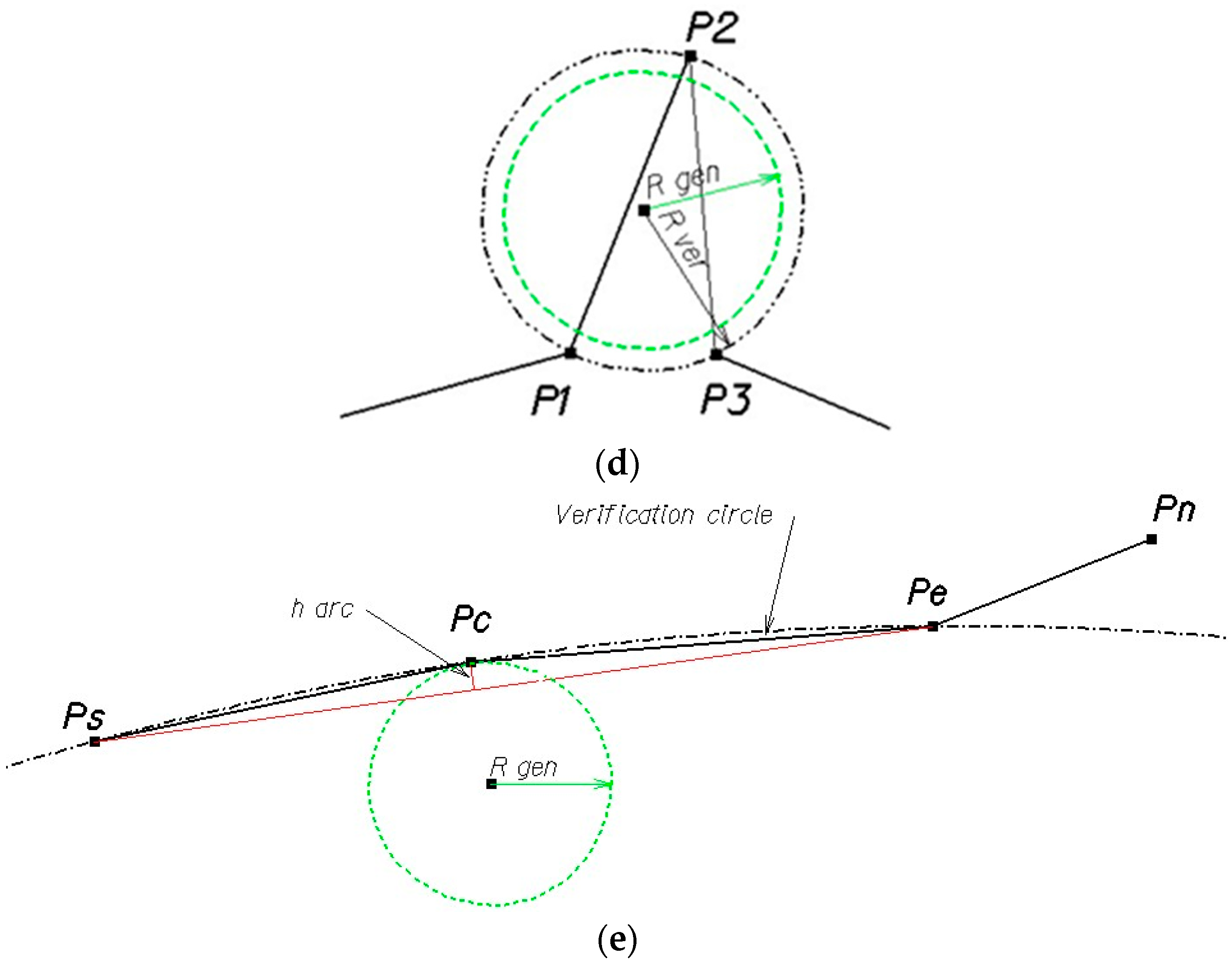
- if the verification radius is greater or equal to the generalization radius Rver ≥ Rgen (Rwer − Rgen > 0) and ds(PS,PE) < 2 × Rgen, as shown in Figure 1d, then the PC point will be removed from the set of vertices of the vector line or moved in another position in order to smooth the line as explained later. In case that Rver ≥ Rgen and ds(PS,PE) > 2 × Rgen and harc < hdop, the point P3 = PC will be removed from the set of vector line points (see Figure 1e).
- The successive three points are subject to examination starting from P2;
- in the same way, all the points of the vector line are analyzed in the first iteration stage. The result of the first stage of generalization is shown in Figure 2;
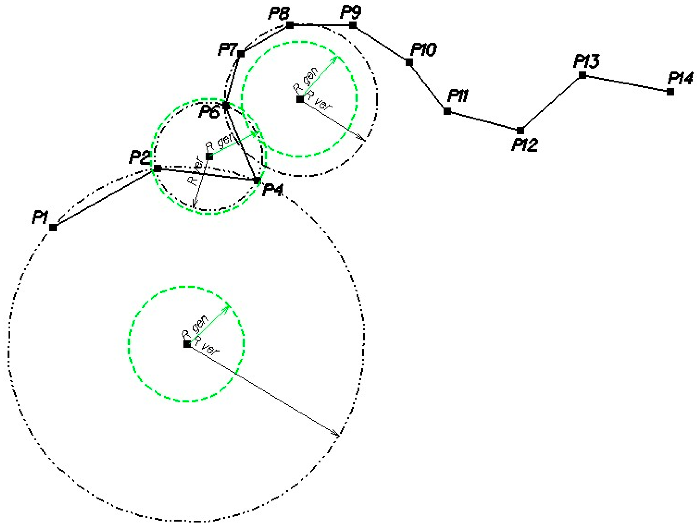
- in the second iteration stage, the radius values of circles based on the remaining points of the vector line are checked again starting from point P1. This situation is illustrated in Figure 3. In this case, the radius of the circle circumscribed on P2 = PS, P4 = PC, and P6 = PE is shorter than the radius of generalization, so the point P4 will be removed from the set of vertices of the vector line;
- The generalization process continues until the position of the last point in the vertices line is evaluated. If the number of vertices has been reduced in the process, iteration begins, starting from point 1. A new set of vertices is subject to generalization. This iterative generalization lasts until iteration does not cause a change in the number of vertices. The lack of further changes in the number of vertices is a condition whose fulfilment ends the procedure of the algorithm (interruption of iteration); and,
- after the completion of the generalization process, the vector line will take the form shown in Figure 4.
An important issue to determine the value of the initial radius of generalization, which will be the basis for determining the degree of simplified polyline. We refer to the vector lines that are contained on the map. Map lines are an approximation of empirical curves that have already been generalized by surveyors or GIS system operators in the process of spatial data acquisition. The principle applied to large-scale maps for the purposes of measuring objects having boundaries in the form of curves consists in selecting measurement points in such a way that the distance of the chord, based on two subsequent points to the arc, is not greater than the acceptable error of determining the coordinates of this element, whose value for analogue topographic maps is 0.3 mm × Mmap (Mmap—denominator of the map scale).
4. Evaluation of the Proposed Generalization Algorithm
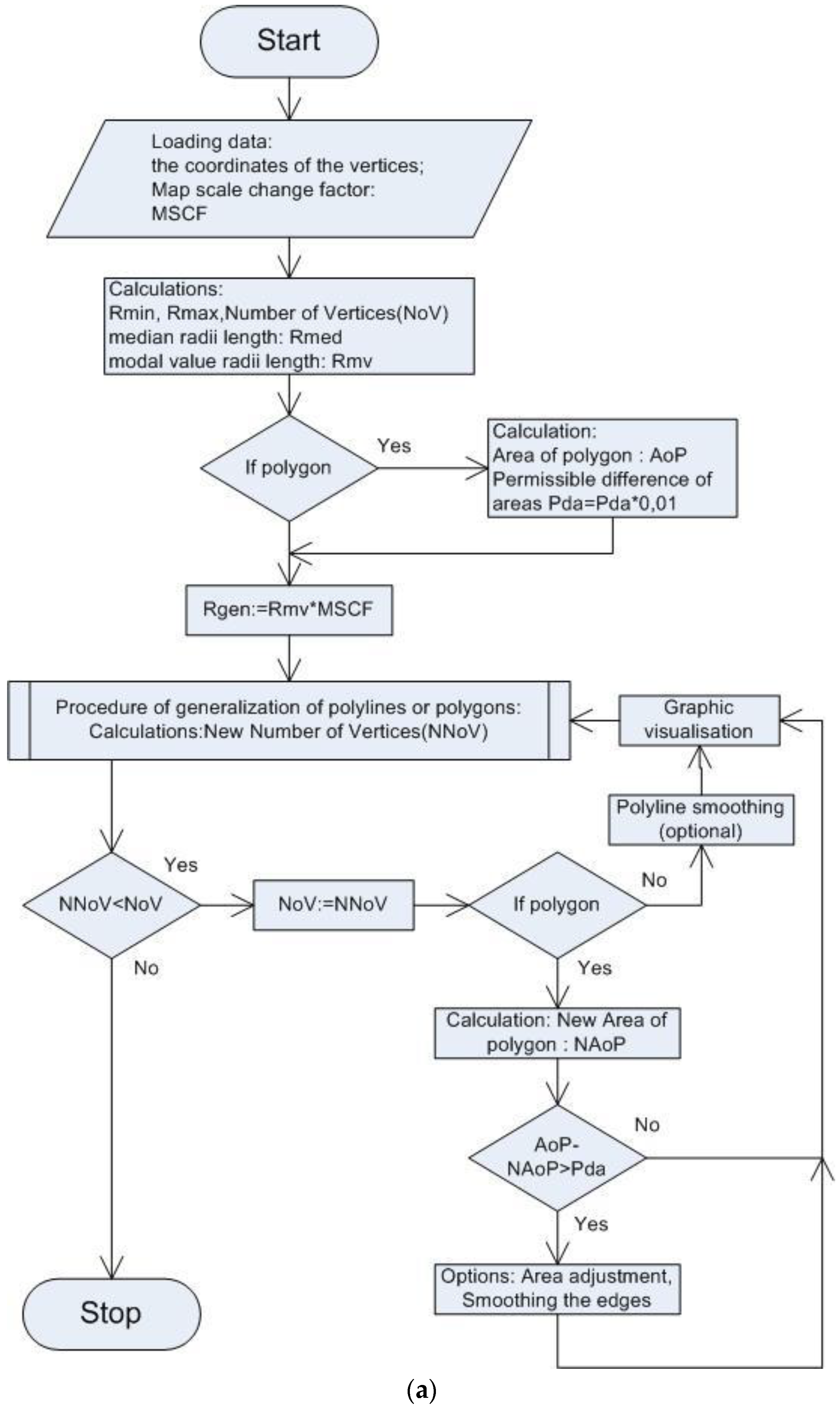
In order to investigate the operation of the vector line generalization algorithm, based on the analysis of the radius of curvature, a computer program in Delphi language was written. A simplified block diagram of the program has been presented in Figure 4a. The input data for the program are: the coordinates of the points forming the vertices of the vector line (polyline) or the coordinates of points of the area (polygon) and the Map Scale Change Factor (MSCF). MSCF is an empirical coefficient that is used to calculate the value of the radius of generalization depending on the map scale value and the modal value of empirical radii of three consecutive vertices on a vector line:
where: MSCF—Map Scale Change Factor—empirical coefficient used to calculate the value of the radius of generalization depending on the map scale value and the modal value of empirical radii of three consecutive vertices on a vector line; Mn—scale of the newly developed map; Ms—scale of the source map; and, hemp—empirical coefficient used to adjust the generalization radius to the modal value and scale of the newly developed map. Based on the analyses of the shape of generalized lines that were obtained in several tens of experiments and the analyses of the error in the adjustment of lines after generalization (see Section 5), the value of 0.3 was adopted. The aim of the value of this coefficient is also to achieve the most aesthetic acceptable generalization in a significantly reduced scale; C1—proportionality coefficient that ensures that the MSCF value is higher than one (C1 = 1).
The modal value and the MSCF factor values constitute the basis for calculating the Rgen generalization radius.
where: Rmv—radii modal value.
The determination of the MSCF coefficient was one of the most important issues that determined the quality of the obtained solutions. The aim of the Authors was to link the generalization process to the change in the scale of the topographic map. The idea that is known from the Tobler formula [5] was used here. The adopted basis for the generalization coefficient is the ratio of the source map scape to the resulting map scale. If the scale of the map remains unchanged, i.e., Mn/Ms = 1 the generalization process should not be conducted. This is a limitation of the scope of generalization conducted with use of this method.
The presented algorithm was developed based on the assumption that it would be used to generalize physiographic lines. This assumption hinders the determination of the appropriate value of the main parameter that controls generalization in this method, i.e., the radius of generalization. It determines the degree of simplification of the vector line. The proposed method of simplification of a vertex line is iterative while maintaining a constant radius of generalization, whose length depends on the degree of change in the scale of the map. The value of Rgen, calculated based on the MSCF coefficient and the modal value of the radii, links the map scales to the shape of the vertex line and it is applicable only if the algorithm is applied to topographic maps. To determine its value, we used indices in form of the generalization error that consists of two values apart from the visual assessment of the generalized line. The error resulting from the use of the smoothing function (Msm) was calculated based on the differences between the values of the co-ordinates of vertices before and after generalization. Coordinates of vertices that remained after the reduction were used for calculations. Some of them had been subjected to the smoothing procedure and for polygons—the surface had been evened, which led to a change in their position.
where: MP—error in vertex position after generalization, caused by the application of smoothing function; MX—error in the determination of the X coordinate; MX—error in the determination of the Y coordinate; ΔXi—difference between coordinates after and before generalization: ΔXi = Xi′ – Xi; ΔYi—difference between coordinates after and before generalization: ΔYi = Yi′ – Yi; Xi, Yi—coordinates of the ith vertex before generalization; Xi, Yi—coordinates of the ith vertex before generalization; and, n—number of vertices remaining after generalization.
The second component of the generalization error is the error resulting from the reduction of vertices. For the purposes of the algorithm, a procedure was used that calculated the Hausdorf distance between the removed point Pc (the middle point of the three) and the line connecting points Ps and Pe (the start and end points). These values were used to calculate the value of the line position error after generalization, pursuant to the formula:
where: MRed—line position error after the reduction of vertices; DH—Hausdorf distance between the line and the reduced vertex; and, l—number of reduced vertices (l ≠ 1).
Generalization error was calculated with use of the formula:
where: Mgen—generalization error.
The results of error calculations for each of the four datasets (shown in Figure 5c, Figure 6a, Figure 7a and Figure 8a) are presented in Table 2 in Section 5. The errors were calculated for each generalization process with a change in the map scale. The results of the preceding generalizations constituted input data for subsequent ones.
In the beginning, the algorithm calculates the initial parameters: the number of vertices, the radii of the circles based on subsequent sets of three vertices, minimum and maximum circle radii, and the median and the modal value of the series. The legitimacy of the statistical position indicators that were adopted for analysis is presented in Section 5. For closed vector lines (polygons), the surface area is calculated. For research purposes, the software was equipped with procedures that enable variant-based realization of the algorithm. The options of line smoothing and (for polygons) evening the surface may be used. The computer program was also equipped with a procedure of graphic visualization of input spatial data and consecutive stages of generalization.
At the first stage of its operation, the computer program that is based on the algorithm that realizes Formula (2) performs a reduction of the vertices of the polyline or polygon by analysing the vertices from the first one to the last one on the whole line. After the end of the iteration, at the next stage of generalization, if the number of vertices after the iteration is lower than before (i.e., if the number of vertices has been reduced), the vector line (polyline) is subjected to the smoothing procedure. It was the intention of the authors for the shape of the processed line to be as close to that of empirical (physiographic) lines as possible. To achieve it, smoothing was applied apart from the functions of the reduction of the number of vertices, and, for closed polygons, their surface was evened. Smoothing is applied to these vertices that fulfil condition 3 in Formula (2). If the smoothing function is active, then these points are not removed, but are moved to a position on the arc of the generalization circle, spanned between the starting and ending points of the analysed three points (Figure 5b).
If the analyzed line is the border of an area, then the surface of the area is additionally aligned after the iteration. The centroid of the shape that is formed by the area border has been adopted as the invariant of the transformation of vertices. The procedure involves checking whether the difference between areas before and after iteration does not exceed the permissible value (Mda). If it does, then the position of vertices is changed according to the direction of their distance from the center of gravity. The algorithm of the surface adjustment function is based on calculating the changes in the distances between the center of gravity of the polygon (the centroid) with specific vertices, proportionally to the length of the vector line. The algorithm is iterative, so, after the calculations are completed, the difference in the surface of the areas is verified again. If the difference between the areas still does not meet the assumed condition, then the procedure of changing the position of vertices is repeated until satisfactory results are obtained (i.e., until the difference is smaller than acceptable). The acceptable difference (Mda) was adopted as 0.01 of the initial value of the area. In the further stage of the generalization process, the number of vertices is again reduced and the difference in the surface areas is re-checked. This step is repeated until the number of vertices remains unchanged in a subsequent iteration.
The illustrations below present the input data and generalization results. Figure 6a,b show the shape of an open vector line (polyline) before and after generalization. This is a test dataset that allows for a graphic presentation of the generalization principle. It does not show the real object and it illustrates the effectiveness of the algorithm in reducing the number of vertices and simplifying the shape. The presented drawings were developed with use of the procedure “Draw a polygon” implemented in the application.
The visualization procedure transforms the input coordinates from the geodetic (Cartesian) set of coordinates to the set of coordinates of the computer screen. This is a simple procedure that uses the graphic components of the Delphi language to draw vertices and the lines that connect them. The drawing is updated after each iteration.
Figure 6c–e show stages of generalization of a vector line that are a result of the vectorization of the coastline of a river section. The scale of the source map was 1:25,000, and of the target maps—1:50,000 and 1: 100,000. In the case shown in Figure 6d the modal value of the statistical series of the vertices dataset was 65. The adopted value of the generalization radius Rgen = 104 m was calculated with use of Formulae (5) and (6). In the case shown in Figure 6e, the modal value of the statistical series of the vertices dataset was 105 m. The adopted value of the generalization radius Rgen = 168 m was calculated with use of Formulae (5) and (6).
It should be noted that, when this method of generalization is used, the algorithm requires performing it consecutively, for each map scale, from larger to smaller ones. The results of generalization in the larger scale, recorded in files on computer disc, constitute input data for the generalization of the map in a smaller scale in the adopted series of scales. This procedure has been used in each of the generalization cases presented below.
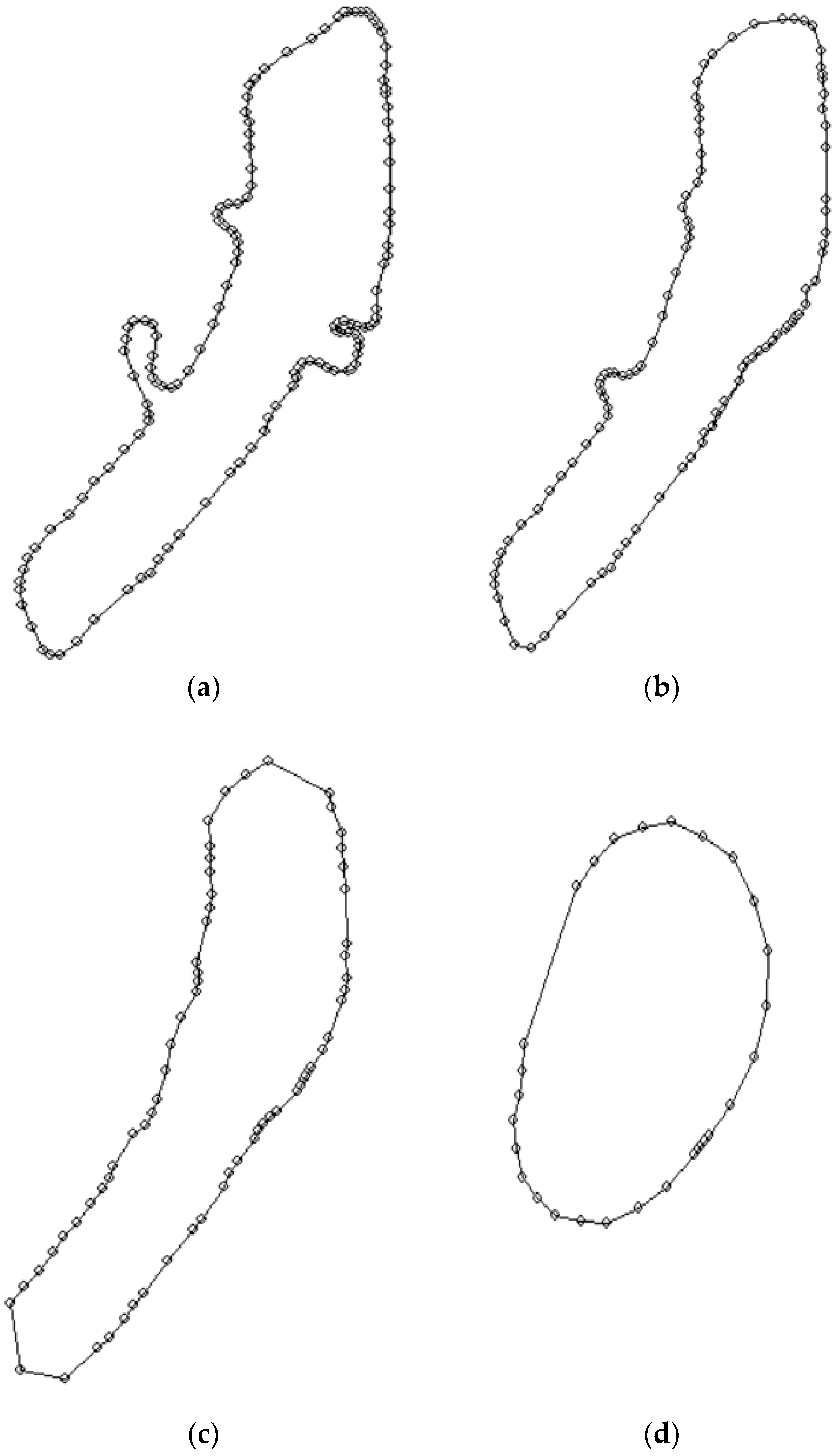
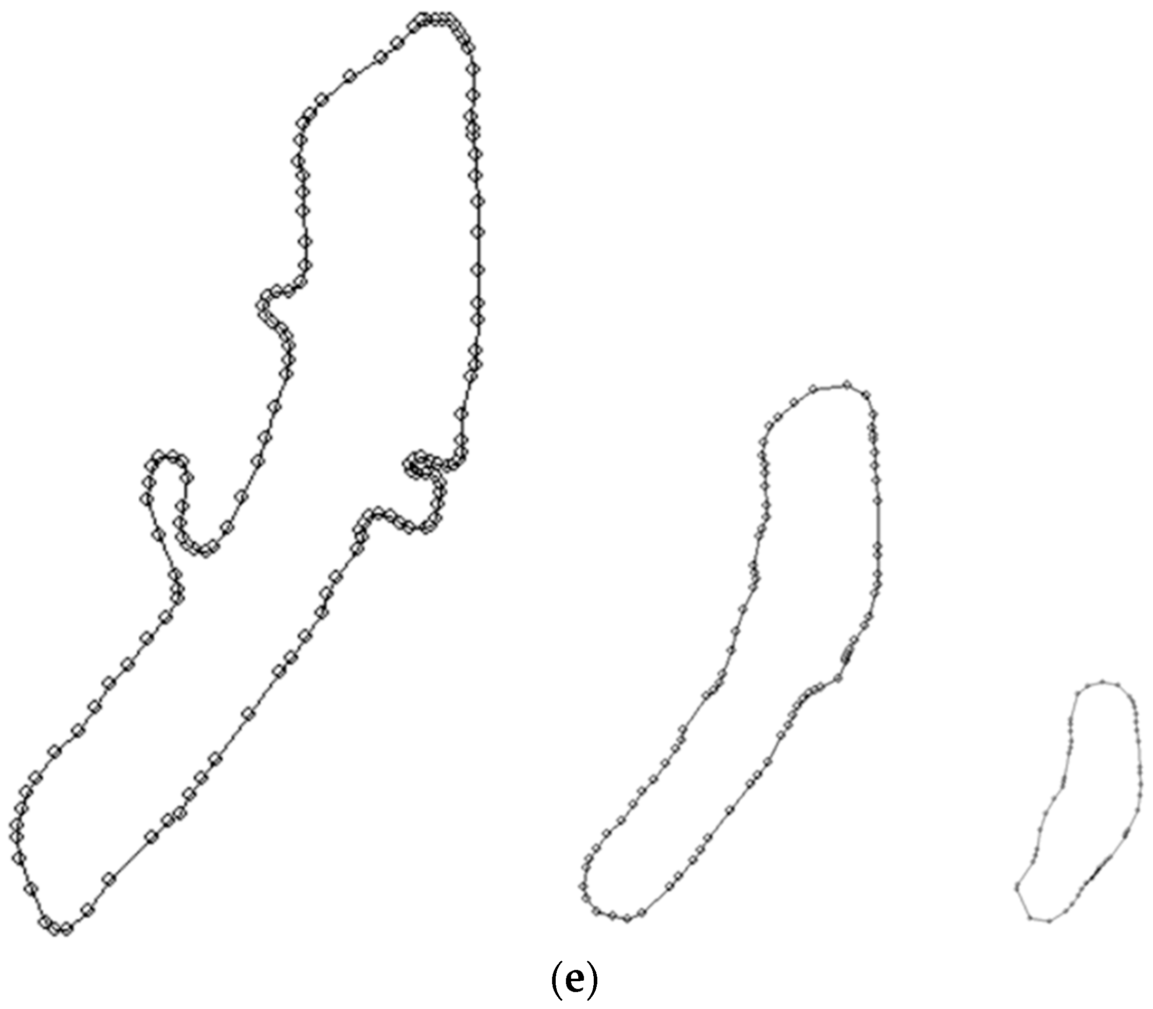
Other types of vector lines were also subjected to the algorithm. One of them is shown in Figure 7a–e. Generalization was applied to a closed vector line, whose shape was obtained as a result of vectorization of the coastline of a water reservoir contained in the topographic map in the scale of 1:25,000. The aim of generalization was to obtain a form of the vector line that would be suitable for application in the process of generalization of a map in the scale of 1:50,000. Figure 7b shows the result of generalization with the modal value of 25 m used as the adopted generalization radius and the MSCF coefficient of 1.6. The operation of the program ended when no changes in the number of vertices occurred in subsequent iterations. The number of vertices of the vector line decreased from 141 to 89.
Figure 7c presents the result of generalization with the applied modal value of 44 m, which, according to Formulae (5) and (6) and the MSCF factor of 1.6, resulted in the Rgen generalization radius of 71 m. Iterations were finished when no further changes occurred in the number of vertices, which was reduced to 56. The aim of this attempt was to generalize the object for a map in the scale of 1:100,000. Figure 7d shows the result of an attempt at the application of the generalization radius of 130 m (modal value—74 m, MSCF 1.75) for further generalization of the object for a map in a scale of 1:250,000. Iterations were finished when no further changes occurred in the number of vertices, which was reduced to 27. Subsequent iterations did not lead to a further reduction.
Figure 7e presents source data in the scale of 1:25,000 and the results of the operation of the generalization algorithm on approximate map scales: 1:50,000 and 1:100,000 in the way, in which they would be presented on such maps.
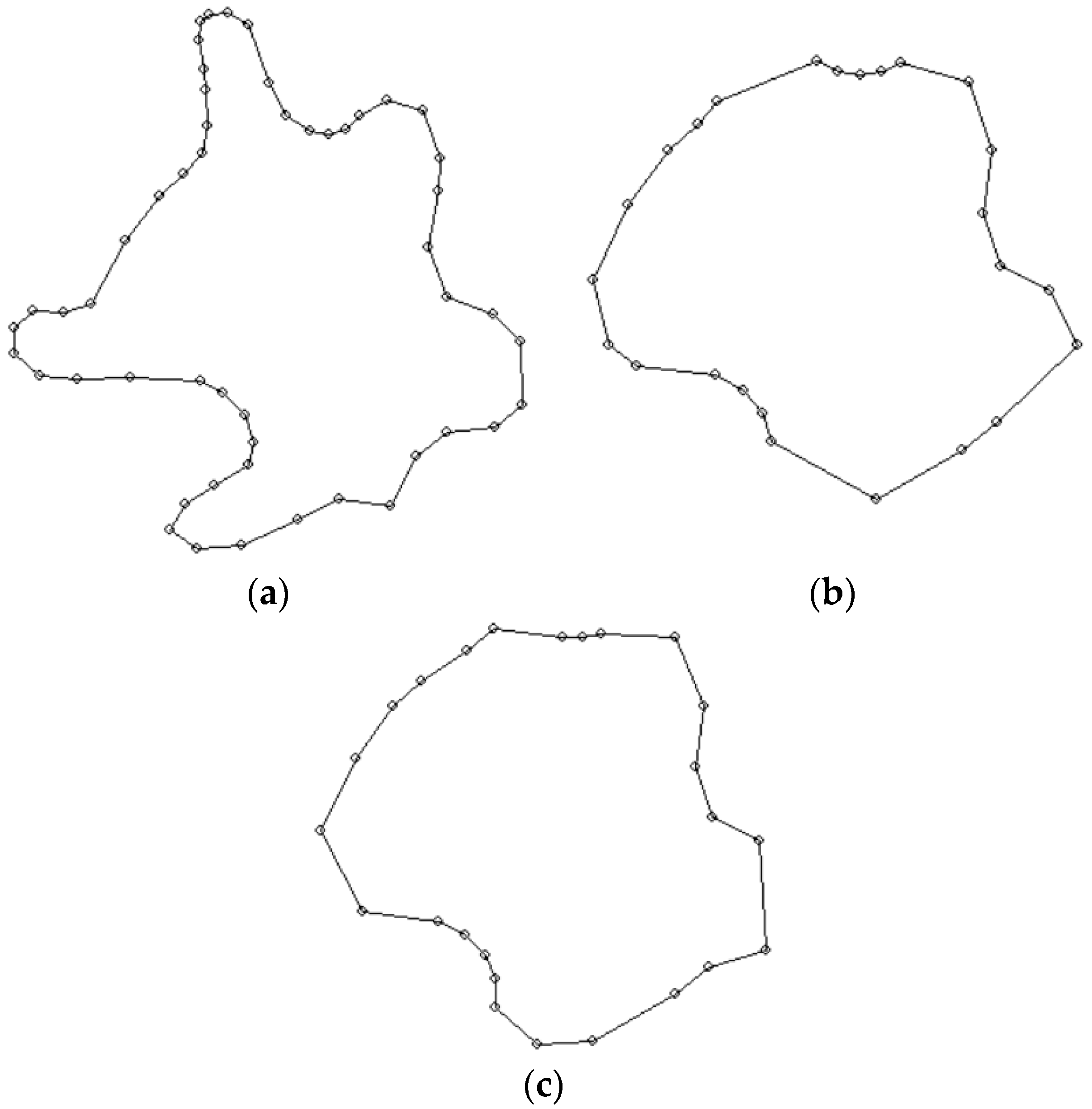
Another example of closed vector line generalization is the shape presented in Figure 8a,b. As in the previous example, the radius based on the modal value of the data series (modal value—26 m, MSCF—1.6) was adopted as the generalization radius from scale of 1:25,000 to the map scale of 1:50,000. Iterations ended when there were no further changes in the number of vertices, which diminished to 25. A similar shape is presented in Figure 8c. The aim of this generalization attempt was to obtain the object shape that would be suitable for a map scale of 1:100,000. The Rgen radius was 67 m, pursuant to Formulae (5) and (6). Iterations were ended when the number of vertices of the vector line decreased to 19 and did not diminish any further.
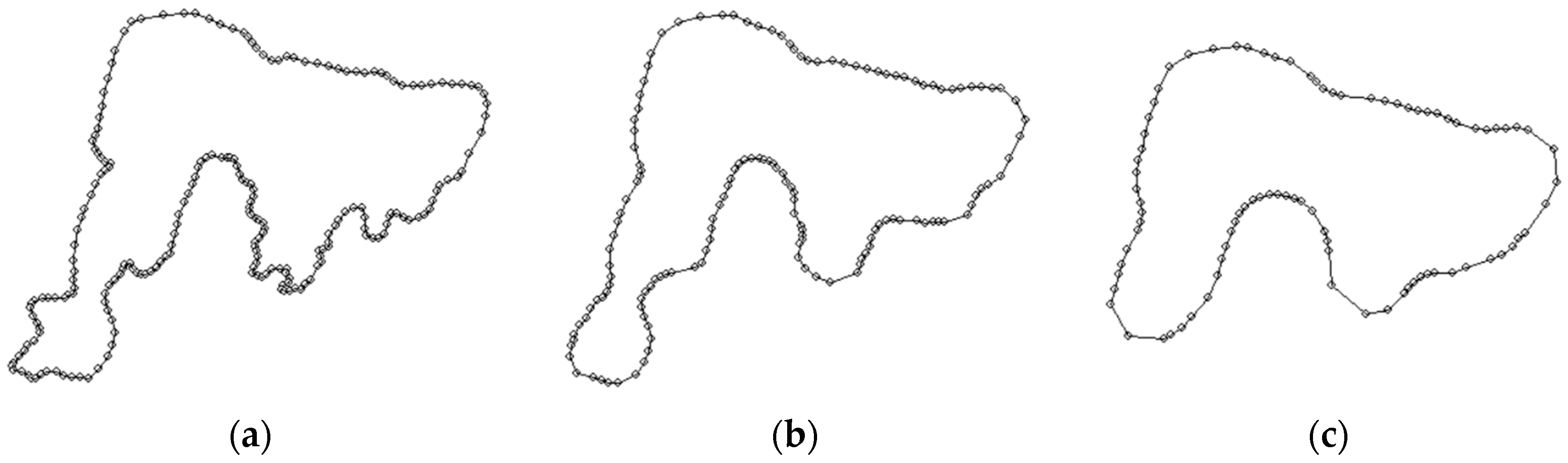
Another example of closed vector line generalization is the shape that is presented in Figure 9a,b. As in the previous example, the radius of 22 based on the modal value of the data series (modal value—14, MSCF—1.6) was adopted as the generalization radius from scale of 1:25,000 to the map scale of 1:50,000. Iterations ended when there were no further changes in the number of vertices, which diminished to 142. A similar shape is presented in Figure 9c. The aim of this generalization attempt was to obtain the object shape that would be suitable for a map scale of 1:100,000. The Rgen radius was 40 m, pursuant to Formulae (5) and (6). Iterations were ended when the number of vertices of the vector line decreased to 89 and they did not diminish any further.
The results of vector line generalization based on this algorithm were compared with the Douglas-Peucker algorith [7] For that purpose, an application in the C++ language was used, whose source code is presented on the website https://rosettacode.org/wiki/Ramer-Douglas-Peucker_line_simplification. The application was compiled in online mode with the use of the compiler that is available on the website https://www.onlinegdb.com/online_c++_compiler.
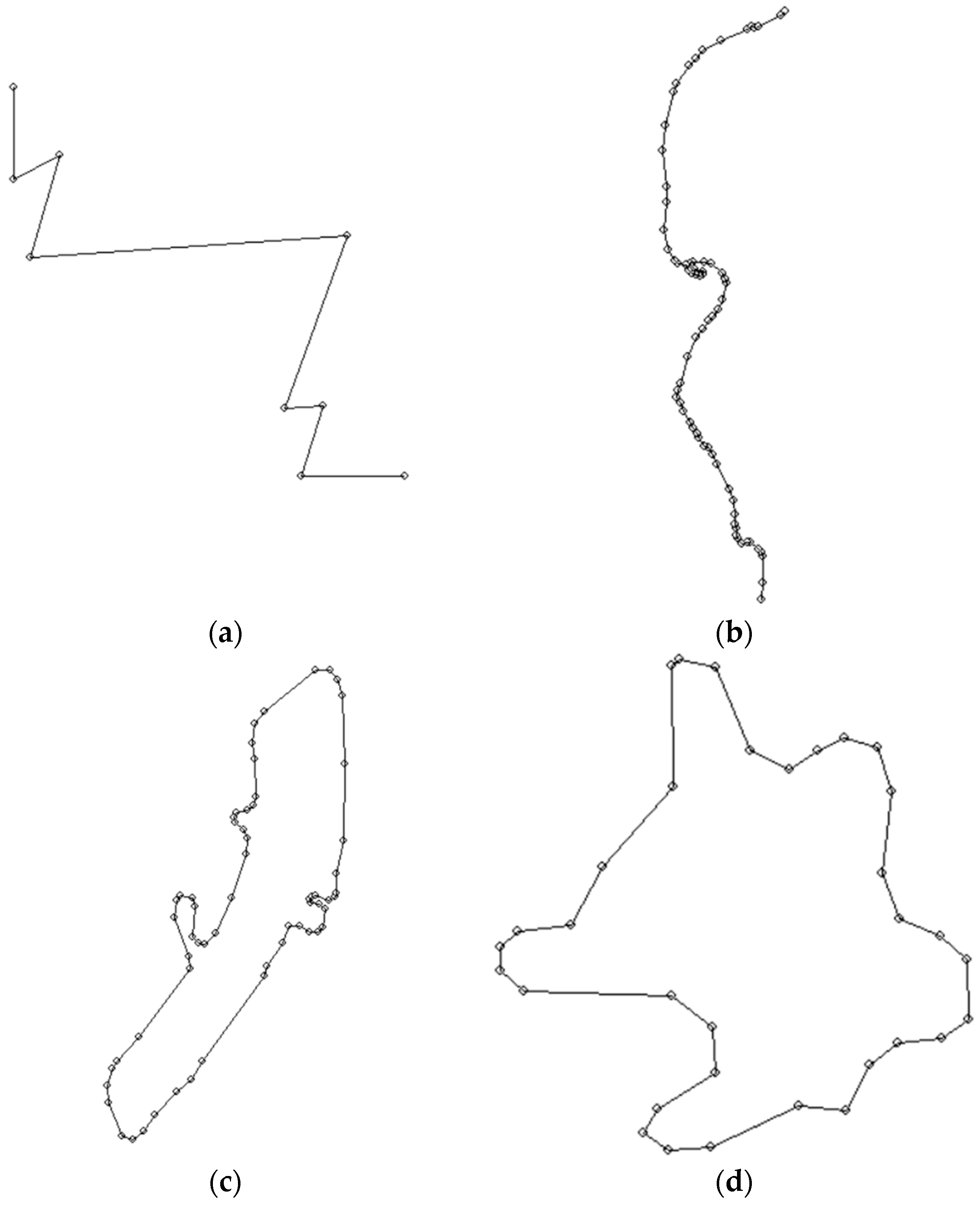
The main problem in the comparison of these algorithms was the determination of the value of the reduction parameter that was used in the Douglas-Peucker method, and more specifically, the determination of its dependence on the scale of the generalized map. The Douglas-Peucker algorithm is a method of reducing the number of vertices. None of the vertices change its position. Figure 10a–d present the results of the reduction of datasets shown, respectively, in Figure 6a,c Figure 7a and Figure 8a. It is difficult to compare the reduction and generalization results, as the operation of the algorithms is based on different principles. The aim of the algorithm that was proposed by the authors is to introduce such changes to the set of vertices that will not only reduce their number, but also change the position of some of them. These changes result from the operation of the smoothing function, which is used in order to maintain the topographic nature of the line. Another reason for changing the position of vertices is to adjust their positions to the optimum position, so that the acceptable difference in the surface areas of polygons is not exceeded. The authors propose to use 1/10 of the modal value of the series of verification radii as the reduction parameter in the Douglas-Peucker algorithm.
5. Discussion
An important parameter of the proposed generalization process is the size of the radius of the generalization circle, at which the optimum shape of the line and number of vertices of the vector line are achieved for the subsequent map scale in the series of scales. Polish analogue topographic maps use scales from 1:25,000 to 1:50,000, 1:000,000, and 1:250,000 in compliance with NATO standards. Assuming that the initial generalization of line shape takes place during the determination of the coordinates of the vertices (e.g., during field measurements or vectorization of orthoimaging) and that it is performed by a surveyor or GIS operator, it is reasonable to assume that the size of the error of the determination of such coordinates is proportional to and compliant with the general principles of generalization of curved lines (empirical curves). The principle states that the difference between the position of the point on the curved line and the chord based on two subsequent vertices of the vector line cannot exceed the error of the position of the determined element that is permissible for the given map. This difference increases with the growth of the scale denominator. The analysis of various shapes of curves that are approximated with vector lines demonstrates the connection between the new, smaller map, with the modal value of the lengths of the radii of circles being based on three consecutive vertices. Adapting the generalization radius calculated for the given scale of the target map according to Formulae (5) and (6) results in a significant reduction in the number of vertices, while the fidelity of the shape of the line after generalization to the original shape is maintained.
The presented method of determining the generalization radius directly depends on the change in map scale (Formula (5)). While developing the algorithm, the authors assumed that its results should reflect the cartographic method of editing maps when changing their scale from large to small. The parameter that controls generalization that was used for the evaluation of the algorithm in tests was one of the statistical indicators of the position of the elements in data series. Treating the determination of the position of vertices of the vector line in a simple vector model as a measurement experiment performed in the field or on the computer screen during vectorization, it was considered that the lengths of the radii of circles defined by three consecutive points are variables that constitute a statistical series. Apart from the influence of the methodological and equipment-related conditions, each result of measurement that is performed by an observer in the process of field or laboratory generalization is also affected by the individual personal traits of the observer. These traits are of a random nature. Due to that, one may attempt to describe the resulting statistical series with use of the statistical position indicator. This indicator depends not so much on the distance between consecutive vertices of the line, but also on their position in relation to each other. This is why this series is called a statistical shape series, as, according to this algorithm, the “co-linearity” of three consecutive vertices of the vector line is an important element that controls generalization.
To assess the usability of location indices that can be used in assessing the validity of generalization, we tested the use of dominant, median, and average radii of circles as factors enabling the determination of the radius of the generalization. These statistics are presented in Table 1. Four datasets (shown in the Figure 5c, Figure 6a, Figure 7a and Figure 8a) were analyzed and accordingly these data were grouped in Table 1. Data set number 1 applies to a linear object (polyline), while the rest relates to areas (polygon). The data contained in the table show that with the implementation of subsequent generalizations for individual map scales, in each data set the same relationships between the basic statistical indicators are observed.
Conducting generalization for subsequent map scales results in a proportional increase in the calculated median and modal value of the radii of verification circles.
With the increase of the radius of generalization, the number of vertices decreases and the average radius of circles that are based on successive points of the line increases. This trend is noticeable in each set of analyzed data. Similar changes were observed for statistical indicators (median and modal value).
The table contains a list of calculated mean squared errors of the position of vertices after generalization. The column marked as Mp_map contains the values of acceptable errors in the position of points on maps in the analyzed scales, pursuant to the hdop value that is specified in Formula (2). Column Msm1 presents the values of smoothing errors calculated pursuant to Formula (7), where measurement data or the results of previous generalization were used as the initial values of coordinates. The initial values of coordinates were adopted for calculations as error-free. Each calculated error value was referred to the adopted map scale. Column Mred1 contains the values of reduction errors calculated pursuant to Formula (10). The calculations were based on the value of the Hausdorf distance between the removed vertex and the chord connecting the start and end points of the analyzed three vertices. Each calculated error value was referred to the adopted map scale.
Columns Msm2 and Mred2 contain, respectively, the errors calculated while considering the erroneous positions of points obtained from the previous M generalizations where error for generalization j is equal to MP1i, pursuant to the formula:
where: Mp2 refers, respectively, to Msm2 and Mred2 errors.
Columns marked as Mgen1 and Mgen2 present the values of generalization errors, described as:
where: i—error index in the specific column of Table 2.
Error values are an indicator of generalization quality. The values that are contained in the table demonstrate that the generalization error increases with the increase in the generalization radius (adequately to the map scale denominator. In one case (dataset No. 3, generalization from map scale 1:100,000 to scale 1:250,000), it slightly exceeds the acceptable values of point position error for the relevant map scale. These results demonstrate that the assumptions set for the developed algorithm have been fulfilled, i.e., that the simplified shape of vector lines subjected to subsequent generalizations has been maintained and thee error in developing a topographic map in the given scale has not been exceeded.
In order to evaluate the usability of potential indicators, we have tested the use of modal value, median, and average of the radii of circles as the factors that enable the determination of the length of the objective generalization radius. The authors understand the objectivity of the applied generalization method as becoming independent from the individual habits of cartographers-editors. Each of such cartographers-editors, although they comply with the same principles during the generalization of shapes, does it in an individual, subjective way. Due to the extensive and complex data resources in topographic maps, the principles of editing such maps are in some instances quite general. This allows, for example, to determine the shape of linear objects quite freely. Another aim of the application of the proposed algorithm is to increase the degree of automation of the analogue map editing process on the stage of developing their digital form. Analogue maps (cartographic versions of maps in digital format) are the final stage of the technological process of their creation. In simple terms, their development consists of several stages:
- obtaining spatial data and recording them in an IT system, usually GIS;
- complementing their characteristics with descriptive data;
- creating a cartographic data base; and,
- processing it to obtain a topographic analogue map in the desired scale.
It is possible to use the algorithm at the final stage of developing a topographic map, during the reparation of the so-called “carto output”. The tool used for creating, updating and editing topographic maps is GIS software, such as ArcGIS® by ESRI or Geomedia® by Intergraph. The language of the internal applications in GIS systems is the currently very popular Python language. For the purposes of using this generalization method in these software systems, an application in the Python environment should be developed.
The results of these attempts presented in Figure 5a to Figure 7d demonstrate that the statistical indicator of a data series that reflects the nature of the generalized line best is the modal value of this series. Figure 5a,b present a quite simple example of a vector line with a small number of vertices. It does not show any actual field object and it illustrates the effectiveness of the algorithm in reducing the number of vertices and simplifying the shape. The line (polyline) that is presented in Figure 5c,d is a result of the vectorization of a river coastline. It was subjected to generalization with use of a simple smoothing function based on the principle of moving certain vertices onto the circle of the generalization radius.
Both the indicator of the reduction of the number of vertices of the vector line and the shape of vector line obtained after generalization, which reflects its original shape quite correctly, prove that the application of this indicator was justified. Figure 5d,e and Figure 6f show generalized shapes of vector lines in printout scales. This enables comparing the quality of the algorithm in terms of maintaining the characteristics of the vector line.
The computer application was also equipped with an option that enables comparing the difference in the surface area of the polygon before and after generalization. The authors developed an iteration algorithm that adjusts the position of points after generalization, so that the difference between the area enclosed by the line after the reduction of vertices and the initial area does not exceed the assumed error in the determination of surface area. The invariant of the coordinates’ re-calculation process is the position of the centroid of the figure created by the polygon. Figure 6d shows the generalization of polygon shape after generalization adequate for analogue map scale of 1:250,000. The surface area is similar to the initial one, and the shape approximates an oval, which, in further iterations, may be approximated by a circle.
6. Conclusions
The presented generalization method was designed as a tool to be used mainly for processing digital data during the process of compiling analogue (cartographic) maps. Cartographic compiling of topographic maps is a labor consuming and individualized stage of working on maps in a scale smaller than the initial scale. Each such map has some properties that are characteristic for the person who performs the editing. As a result, each map is unique and subjective. The proposed algorithm by definition automates and facilitates the process of simplification and the reduction of linear elements of the map. Its main property consists in the objective reduction of vertices of lines, while at the same time maintaining a high degree of similarity between the generalized elements. The algorithm fulfils the condition stating that nodal points of the set of lines cannot be subject to changes (removal or displacement).
In order to test the operation of the algorithm, a computer program in the Delphi language was developed. Apart from realizing the functions of reduction and simplification of the vector lines, it also smoothens them, and for areas that are delimited by vector lines it performs the procedure of the adjustment of the position of vertices in order to maintain their surface areas relatively stable. The conducted tests of the operation of the algorithm in the form of a computer program allow for us to state that:
- the design of the algorithm does not require complicated programming solutions to implement it in GIS systems;
- the algorithm may be applied both to polylines and to vector lines that constitute the borders of areas. The algorithm works best for such physiographic elements of the map as water courses, land/water borders, borders of forest complexes etc.; and,
- the following points do not change their position and they are not subject to reduction during generalization: the start and end of the polyline, the center of gravity of the figure constituting the area and selected points marked in the dataset.
Based on the tests and analyses conducted so far, we believe that it is justified to conclude that the presented algorithm is well-suited for the generalization of vector lines in computerised systems of digital maps. However, its application and further testing in GIS systems must be preceded by translating the computer application from the Delphi language to the language that is used by the applications of those systems, e.g., Python.
Author Contributions
B.K. and D.L. developed and designed the study; J.A. analyzed the results and developed a summary of the research; B.K. conducted experiments and wrote an article; B.K., D.L. and J.A. read and accepted the manuscript.
Funding
The research was carried out as part of the statutory work “Acquisition and processing of geodata for the purposes of national security and defense” implemented in 2015–2018 at the Military University of Technology in Warsaw, Poland.
Conflicts of Interest
The authors declare no conflict of interest.
References
- Kraak, M.J.; Omerling, F. Kartografia; PWN: Warszawa, Poland, 1998. [Google Scholar]
- Saliszczew, A.K. Kartografia Ogólna; PWN: Warszawa, Poland, 1984. [Google Scholar]
- Magnuszewski, A. GIS w Geografii Fizycznej; Wydawnictwo Naukowe PWN: Warszawa, Poland, 1999. [Google Scholar]
- Robinson, A.; Sale, R.; Morrison, J. Podstawy Kartografii; PWN: Warszawa, Poland, 1988. [Google Scholar]
- Tobler, W. Numerical map generalization. Mich. Inter-Univ. Commun. Math. Geogr. 1966, 8, 25. [Google Scholar]
- Iwaniak, A.; Paluszyński, W.; Żyszkowska, W. Generalizacja map numerycznych - koncepcje, narzędzia. Polski Przegląd Kartograficznyc 1998, 30, 79–88. [Google Scholar]
- Douglas, D.H.; Peucker, T.K. Algorithms for the reduction of the number of points required to represent a digitized line or its caricature. Can. Cartogr. 1973, 10, 112–122. [Google Scholar] [CrossRef]
- Li, Z.; Openshaw, S. Algorithms for automated line generalization based on a natural principle of objective. Int. J. Geogr. Inf. Syst. 1992, 6, 373–389. [Google Scholar] [CrossRef]
- Visvalingam, M.; Whyatt, J. Line generalization by repeated elimination of points. Cartogr. J. 1993, 30, 46–51. [Google Scholar] [CrossRef]
- Wang, Z.; Muller, J.-C. Line generalization based on analysis of shape characteristics. Cartog. Geogr. Inf. Syst. 1998, 25, 3–15. [Google Scholar] [CrossRef]
- Jiang, B.; Nakos, B. Line Simplification Using Self-organizing Maps. In Proceedings of the ISPRS Workshop on Spatial Analysis and Decision Making, Hong Kong, China, 3–5 December 2003. [Google Scholar]
- Zhou, S.; Jones, C. Shape-aware Line Generalisation with Weighted Effective Area. In Developments in Spatial Data Handling; Springer: Berlin/Heidelberg, Germany, 2004; pp. 369–380. [Google Scholar]
- Dyken, C.; Daehlen, M.; Sevaldrud, T. Simultaneous curve simplification. J. Geogr. Syst. 2009, 11, 273–289. [Google Scholar] [CrossRef]
- Saalfeld, A. Topologically consistent line simplification with the Douglas-Peucker algorithm. Cartogr. Geogr. Inf. Sci. 1999, 26, 7–18. [Google Scholar] [CrossRef]
- Mustafa, N.; Krishnan, S.; Varadhan, G.; Venkatasubramanian, S. Dynamic simplification and visualization of large maps. Int. J. Geogr. Inf. Sci. 2006, 20, 273–320. [Google Scholar] [CrossRef]
- Nöllenburg, M.; Merrick, D.; Wolff, A.; Benkert, M. Morphing polylines: A step towards continuous. Comput. Environ. Urban Syst. 2008, 32, 248–260. [Google Scholar] [CrossRef]
- Stanislavski, L.; Raposa, P.; Butterfield, B. Automated Metric Assessment of Line Simplification in Humid Landscapes. In Proceedings of the AutoCarto 2012, Columbus, OH, USA, 16–18 September 2012. [Google Scholar]
- Veregin, H. Quantifying positional error induced by line simplification. Int. J. Geogr. Inf. Sci. 2000, 14, 113–130. [Google Scholar] [CrossRef]
- McMaster, R. The integration of simplification and smoothing algorithms in line generalization. Cartogr. Int. J. Geogr. Inf. Geovis. 1989, 26, 101–121. [Google Scholar] [CrossRef]
- Gökgöz, T.; Sen, A.; Memduhoglu, A.; Hacar, M. A New Algorithm for Cartographic Simplification of Streams and Lakes Using Deviation Angles and Error Bands. ISPRS Int. J. Geo-Inf. 2015, 4, 2186–2204. [Google Scholar] [CrossRef]
- Bose, P.; Cabello, S.; Cheong, O.; Gudmundsson, J.; Van Kreveld, M.; Speckmann, B. Area-preserving approximations of polygonal paths. J. Discret. Algorithms. 2006, 4, 554–566. [Google Scholar] [CrossRef] [Green Version]
- Buchin, K.; Meulemans, W.; Renssen, A.; Speckmann, B. Area-preserving simplification and schematization. J. Discret. Algorithms. 2016, 2, 2. [Google Scholar]
- Perkal, J. Próba obiektywnej generalizacji. Geodezja i Kartografia 1958, 8, 130. [Google Scholar]
- Perkal, J. O długości krzywych empirycznych. Zastosowania Matematyki 1958, 3, 258–284. [Google Scholar] [CrossRef] [Green Version]
- Chrobak, T. Modeling of spatial data in a database for the needs of cartographic generalization. Geodezja i Kartografia 2000, 49, 7–20. [Google Scholar]
- Chrobak, T. Metoda uogólnienia danych w procesie generalizacji obiektów liniowych. Geoinformacja Zintegrowanym Narzędziem Badań Przestrzennych 2003, 13, 15–17. [Google Scholar]
- Chrobak, T. Badania Przydatności Trójkąta Elementarnegow Komputerowej Generalizacji Kartograficznej; Wydawnictwo Naukowo-Dydaktyczne AGH: Kraków, Poland, 1999. [Google Scholar]
Figure 1.
(a) Beginning shape of line string. (b) The first case according to the Formula (1); (c) The second case according to the Formula (1); (d) The third case according to the Formula (2); and, (e) The fourth case according to the Formula (1).
Figure 1.
(a) Beginning shape of line string. (b) The first case according to the Formula (1); (c) The second case according to the Formula (1); (d) The third case according to the Formula (2); and, (e) The fourth case according to the Formula (1).


Figure 2.
The result of the first stage of generalization.

Figure 3.
Advanced stage of generalization.

Figure 4.
Line string after generalization.

Figure 5.
(a) Block diagram of the algorithm. (b) Smoothing the vector line.


Figure 6.
(a) Line string before generalization, initial number of vertexes—15, minimal radius—61 m; (b) Line string after generalization, final form, number of vertexes—8, radius of generalization (modal value × 1.6)—170 m; (c) Line string before generalization, initial number of vertices—125, scale of the map 1:25,000; (d) Line string after generalization, final form, number of vertices—94, radius of generalization (modal value × Map Scale Change Factor (MSCF))—65 m × 1.6 = 104 m, scale of the map 1:50,000; (e) Line string after generalization, final form, number of vertices—80, radius of generalization (modal value × MSCF)—105 m × 1.6 = 168 m, scale of the map 1:100,000.

Figure 7.
(a) Area limited by a polygon, number of vertices—141; (b) Area limited by a polygon, number of vertices—89, radius of generalization (modal value × MSCF)—25 × 1.6 = 40 m. (c) Area limited by a polygon, number of vertices—58, radius of generalization (modal value × MSCF)—44 m × 1.6 =70 m. (d) Area limited by a polygon, number of vertices—29, radius of generalization (modal value × MSCF)—74 m × 1.75 = 130 m. (e) Generalization results presented in approximate map scales: 1:25,000, 1:50,000, 1:100,000.


Figure 8.
(a) Area limited by a polygon, number of vertices—52; (b) Area limited by a polygon, number of vertices—25, radius of generalization (modal value × MSCF)—42 m × 1.6 = 67 m; (c) Area limited by a polygon, number of vertices—19, radius of generalization (modal value × MSCF)—44 m × 1.6 = 70 m.

Figure 9.
(a) Area limited by a polygon, number of vertices—215; (b) Area limited by a polygon, number of vertices—142, radius of generalization (modal value × MSCF)—14 m × 1.6 = 22 m; (c) Area limited by a polygon, number of vertices—89, radius of generalization (modal value × MSCF)—25 m × 1.6 = 40 m.

Figure 10.
(a) Reduction of diagram data (org. Figure 6a), reduction parameter—90 m, number of vertices—9; (b) Line string reduction (org. Figure 6c), reduction parameter—2.1 m, number of vertices—81; (c) Polygon reduction (org. Figure 7a), reduction parameter—2.5 m, number of vertices—62; (d) Polygon reduction (org. Figure 8a), reduction parameter—4.1 m, number of vertices—34.


Table 1.
Summary of statistical indicators of the analyzed data.
| Data Set | Source Map Scale | The Scale of the Target Map | The Type of Object | The Length of the Line [m] | Area Field [m²] | Avg. Side Length | Number of Vertices | Radii [m] | |||||
|---|---|---|---|---|---|---|---|---|---|---|---|---|---|
| Average | Max. | Minimum | Median | Modal Value | Generalization | ||||||||
| No 1 | 1:25,000 | 1:50,000 | polyline | 3867 | x | 29 | 125 | 688 | 17,020 | 1 | 175 | 65 | 104 |
| 1:50,000 | 1:100,000 | polyline | 3845 | x | 38 | 94 | 693 | 8397 | 24 | 236 | 105 | 168 | |
| 1:100,000 | 1:250,000 | polyline | 3580 | x | 38 | 80 | 904 | 8397 | 31 | 281 | 173 | 277 | |
| 1:250,000 | 1:500,000 | polyline | 3454 | x | 43 | 62 | 1030 | 8154 | 42 | 401 | 401 | 702 | |
| No 2 | 1:25,000 | 1:50,000 | polygon | x | 109,244 | 17 | 140 | 260 | 3729 | 1 | 59 | 25 | 40 |
| 1:50,000 | 1:100,000 | polygon | x | 109,173 | 30 | 89 | 415 | 4715 | 21 | 154 | 44 | 70 | |
| 1:100,000 | 1:250,000 | polygon | x | 109,168 | 55 | 58 | 5718 | 51,914 | 71 | 158 | 74 | 130 | |
| No 3 | 1:25,000 | 1:50,000 | polygon | x | 43,600 | 23 | 51 | 128 | 1848 | 11 | 40 | 42 | 67 |
| 1:50,000 | 1:100,000 | polygon | x | 43,599 | 41 | 26 | 111 | 444 | 42 | 68 | 44 | 70 | |
| 1:100,000 | 1:250,000 | polygon | x | 43,598 | 32 | 19 | 301 | 2454 | 66 | 101 | 73 | 128 | |
| No 4 | 1:25,000 | 1:50,000 | polygon | x | 85,607 | 41 | 216 | 106 | 3191 | 3 | 29 | 14 | 22 |
| 1:50,000 | 1:100,000 | polygon | x | 85,053 | 17 | 142 | 121 | 1839 | 21 | 44 | 25 | 40 | |
| 1:100,000 | 1:250,000 | polygon | x | 84,568 | 12 | 89 | 234 | 5123 | 40 | 71 | 55 | 96 | |
Table 2.
List of mean errors of the position of points after generalization.
| Data Set | Source Map Scale | The Scale of the Target Map | The Type of Object | Mp_map | Msm1 | Mred1 | Mgen1 | Msm2 | Mred2 | Mgen2 |
|---|---|---|---|---|---|---|---|---|---|---|
| No 1 | 1:25,000 | 1:50,000 | polyline | 15 m | ±8.4 m | ±21.6 m | ±23.2 m | ±8.4 m | ±21.6 m | ±23.2 m |
| 1:50,000 | 1:100,000 | polyline | 30 m | ±15.0 m | ±1.8 m | ±15.1 m | ±17.2 m | ±21.7 m | ±27.7 m | |
| 1:100,000 | 1:250,000 | polyline | 75 m | ±25.5 m | ±15.1 m | ±29.6 m | ±30.8 m | ±26.4 m | ±40.5 m | |
| 1:250,000 | 1:500,000 | polyline | 150 m | ±44.7 m | ±44.2 m | ±62.8 m | ±54.2 m | ±51.4 m | ±74.8 m | |
| No 2 | 1:25,000 | 1:50,000 | polygon | 15 m | ±12.3 m | ±2.9 m | ±12.7 m | ±12.3 m | ±2.9 m | ±12.6 m |
| 1:50,000 | 1:100,000 | polygon | 30 m | ±13.5 m | ±3.3 m | ±13.9 m | ±18.3 m | ±4.4 m | ±18.8 m | |
| 1:100,000 | 1:250,000 | polygon | 75 m | ±54.7 m | ±19.6 m | ±58.1 m | ±57.7 m | ±20.1 m | ±61.1 m | |
| No 3 | 1:25,000 | 1:50,000 | polygon | 15 m | ±26.3 m | ±7.8 m | ±27.4 m | ±26.3 m | ±21.6 m | ±34.0 m |
| 1:50,000 | 1:100,000 | polygon | 30 m | ±14.2 m | ±2.7 m | ±14.5 m | ±29.9 m | ±21.7 m | ±36.9 m | |
| 1:100,000 | 1:250,000 | polygon | 75 m | ±41.4 m | ±52.3 | ±66.7 m | ±51.1 m | ±56.6 m | ±76.2 m | |
| No 4 | 1:25,000 | 1:50,000 | polygon | 15 m | ±6.4 m | ±1.6 m | ±6.6 m | ±6.4 m | ±1.6 m | ±6.6 m |
| 1:50,000 | 1:100,000 | polygon | 30 m | ±7.3 m | ±8.0 m | ±10.8 m | ±9.7 m | ±8.2 m | ±12.7 m | |
| 1:100,000 | 1:250,000 | polygon | 75 m | ±33.2 m | ±15.5 m | ±36.6 m | ±34.5 m | ±17.6 m | ±38.8 m |
© 2018 by the authors. Licensee MDPI, Basel, Switzerland. This article is an open access article distributed under the terms and conditions of the Creative Commons Attribution (CC BY) license (http://creativecommons.org/licenses/by/4.0/).
Share and Cite
MDPI and ACS Style
Kolanowski, B.; Augustyniak, J.; Latos, D. Cartographic Line Generalization Based on Radius of Curvature Analysis. ISPRS Int. J. Geo-Inf. 2018, 7, 477. https://0-doi-org.brum.beds.ac.uk/10.3390/ijgi7120477
AMA Style
Kolanowski B, Augustyniak J, Latos D. Cartographic Line Generalization Based on Radius of Curvature Analysis. ISPRS International Journal of Geo-Information. 2018; 7(12):477. https://0-doi-org.brum.beds.ac.uk/10.3390/ijgi7120477
Chicago/Turabian StyleKolanowski, Bogdan, Jacek Augustyniak, and Dorota Latos. 2018. "Cartographic Line Generalization Based on Radius of Curvature Analysis" ISPRS International Journal of Geo-Information 7, no. 12: 477. https://0-doi-org.brum.beds.ac.uk/10.3390/ijgi7120477
Note that from the first issue of 2016, this journal uses article numbers instead of page numbers. See further details here.