Checking the Consistency of Volunteered Phenological Observations While Analysing Their Synchrony


Abstract
:
1. Introduction
1.1. VGI Attribute Consistency
1.2. Synchrony of Phenological VGI
2. Materials and Methods
2.1. VPOs and Temperature Datasets
2.2. Analysing Consistency and Synchrony of VPOs
3. Results
4. Discussion
5. Conclusions
Author Contributions
Funding
Acknowledgments
Conflicts of Interest
Appendix A


References
- Beaubien, E.G.; Hamann, A. Plant phenology networks of citizen scientists: recommendations from two decades of experience in Canada. Int. J. Biometeorol. 2011, 55, 833–841. [Google Scholar] [CrossRef] [PubMed]
- Ferster, C.J.; Coops, N.C. A review of earth observation using mobile personal communication devices. Comput. Geosci. 2013, 51, 339–349. [Google Scholar] [CrossRef]
- Ballatore, A.; Zipf, A. A Conceptual Quality Framework for Volunteered Geographic Information. In Spatial Information Theory; Lecture Notes in Computer Science; Springer: Cham, Switzerland, 2015. [Google Scholar]
- Senaratne, H.; Mobasheri, A.; Ali, A.L.; Capineri, C.; Haklay, M. A review of volunteered geographic information quality assessment methods. Int. J. Geogr. Inf. Sci. 2017, 31, 139–167. [Google Scholar] [CrossRef]
- Feick, R.; Roche, S. Understanding the Value of VGI. In Crowdsourcing Geographic Knowledge; Springer: Dordrecht, The Netherlands, 2013; pp. 15–29. [Google Scholar]
- Antoniou, V.; Skopeliti, A. Measures and indicators of VGI quality: An overview. ISPRS Ann. Photogramm. Remote Sens. Spat. Inf. Sci. 2015, II-3/W5, 345–351. [Google Scholar] [CrossRef]
- Arsanjani, J.J.; Mooney, P.; Zipf, A.; Schauss, A. Quality Assessment of the Contributed Land Use Information from OpenStreetMap Versus Authoritative Datasets. In OpenStreetMap in GIScience; Springer: Cham, Switzerland, 2015. [Google Scholar]
- Elwood, S.; Goodchild, M.F.; Sui, D.Z. Researching Volunteered Geographic Information: Spatial Data, Geographic Research, and New Social Practice. Ann. Assoc. Am. Geogr. 2012, 102, 571–590. [Google Scholar] [CrossRef]
- Yanenko, O.; Schlieder, C. Enhancing the Quality of Volunteered Geographic Information: A Constraint-Based Approach. In Bridging the Geographic Information Sciences: International AGILE’2012 Conference, Avignon (France), 24–27 April 2012; Gensel, J., Josselin, D., Vandenbroucke, D., Eds.; Springer: Berlin/Heidelberg, Germany, 2012; pp. 429–446. ISBN 978-3-642-29063-3. [Google Scholar]
- Schlieder, C.; Yanenko, O. Spatio-temporal proximity and social distance. In Proceedings of the 2nd ACM SIGSPATIAL International Workshop on Location Based Social Networks, San Jose, CA, USA, 2 November 2010; ACM Press: New York, NY, USA, 2010; p. 60. [Google Scholar]
- Barron, C.; Neis, P.; Zipf, A. A Comprehensive Framework for Intrinsic OpenStreetMap Quality Analysis. Trans. GIS 2014, 18, 877–895. [Google Scholar] [CrossRef]
- Goodchild, M.F.; Li, L. Assuring the quality of volunteered geographic information. Spat. Stat. 2012, 1, 110–120. [Google Scholar] [CrossRef]
- Haklay, M. How Good is Volunteered Geographical Information? A Comparative Study of OpenStreetMap and Ordnance Survey Datasets. Environ. Plan. B Plan. Des. 2010, 37, 682–703. [Google Scholar] [CrossRef]
- Mooney, P.; Corcoran, P. The Annotation Process in OpenStreetMap. Trans. GIS 2012, 16, 561–579. [Google Scholar] [CrossRef]
- Ali, A.L.; Schmid, F. Data Quality Assurance for Volunteered Geographic Information. In Geographic Information Science; Duckham, M., Pebesma, E., Stewart, K., Frank, A.U., Eds.; Lecture Notes in Computer Science; Springer: Cham, Switzerland, 2014; Volume 8728. [Google Scholar]
- Bonter, D.N.; Cooper, C.B. Data validation in citizen science: A case study from Project FeederWatch. Front. Ecol. Environ. 2012, 10, 305–307. [Google Scholar] [CrossRef]
- Van Vliet, A.J.H.; de Groot, R.S.; Bellens, Y.; Braun, P.; Bruegger, R.; Bruns, E.; Clevers, J.; Estreguil, C.; Flechsig, M.; Jeanneret, F.; et al. The European Phenology Network. Int. J. Biometeorol. 2003, 47, 202–212. [Google Scholar] [CrossRef] [PubMed]
- Mayer, A. Phenology and Citizen Science. Bioscience 2010, 60, 172–175. [Google Scholar] [CrossRef] [Green Version]
- Chmielewski, F.M. Phenology in Agriculture and Horticulture. In Phenology: An Integrative Environmental Science; Springer: Dordrecht, The Netherlands, 2013; pp. 539–561. ISBN 978-94-007-6924-3. [Google Scholar]
- Doi, H.; Katano, I. Phenological timings of leaf budburst with climate change in Japan. Agric. For. Meteorol. 2008, 148, 512–516. [Google Scholar] [CrossRef]
- Gordo, O.; Sanz, J.J. Impact of climate change on plant phenology in Mediterranean ecosystems. Glob. Chang. Biol. 2010, 16, 1082–1106. [Google Scholar] [CrossRef] [Green Version]
- Zurita-Milla, R.; Goncalves, R.; Izquierdo-Verdiguier, E.; Ostermann, F.O. Exploring Vegetation Phenology at Continental Scales: Linking Temperature-Based Indices and Land Surface Phenological Metrics. In Proceedings of the 2017 Conference on Big Data from Space, Toulouse, France, 28–30 November 2017. [Google Scholar]
- Devictor, V.; Whittaker, R.J.; Beltrame, C. Beyond scarcity: citizen science programmes as useful tools for conservation biogeography. Divers. Distrib. 2010, 16, 354–362. [Google Scholar] [CrossRef] [Green Version]
- Ault, T.R.; Schwartz, M.D.; Zurita-Milla, R.; Weltzin, J.F.; Betancourt, J.L.; Ault, T.R.; Schwartz, M.D.; Zurita-Milla, R.; Weltzin, J.F.; Betancourt, J.L. Trends and Natural Variability of Spring Onset in the Coterminous United States as Evaluated by a New Gridded Dataset of Spring Indices. J. Clim. 2015, 28, 8363–8378. [Google Scholar] [CrossRef]
- Rosemartin, A.H.; Denny, E.G.; Weltzin, J.F.; Lee Marsh, R.; Wilson, B.E.; Mehdipoor, H.; Zurita-Milla, R.; Schwartz, M.D. Lilac and honeysuckle phenology data 1956-2014. Sci. Data 2015, 2, 150038. [Google Scholar] [CrossRef]
- Soroye, P.; Ahmed, N.; Kerr, J.T. Opportunistic citizen science data transform understanding of species distributions, phenology, and diversity gradients for global change research. Glob. Chang. Biol. 2018, 24, 5281–5291. [Google Scholar] [CrossRef]
- Ims, R.A. The ecology and evolution of reproductive synchrony. Trends Ecol. Evol. 1990, 5, 135–140. [Google Scholar] [CrossRef]
- English-Loeb, G.M.; Karban, R. Consequences of variation in flowering phenology for seed head herbivory and reproductive success in Erigeron glaucus (Compositae). Oecologia 1992, 89, 588–595. [Google Scholar] [CrossRef]
- Bolmgren, K.; Eriksson, O. Are mismatches the norm? Timing of flowering, fruiting, dispersal and germination and their fitness effects in Frangula alnus (Rhamnaceae). Oikos 2015, 124, 639–648. [Google Scholar] [CrossRef]
- Weis, A.; Kossler, T. Genetic variation in flowering time induces phenological assortative mating: Quantitative genetic methods applied to Brassica rapa. Am. J. Bot. 2004, 91, 825–836. [Google Scholar] [CrossRef] [PubMed]
- Both, C.; Van Asch, M.; Bijlsma, R.G.; Van Den Burg, A.B.; Visser, M.E. Climate change and unequal phenological changes across four trophic levels: constraints or adaptations? J. Anim. Ecol. 2009, 78, 73–83. [Google Scholar] [CrossRef] [PubMed] [Green Version]
- Henderson, A.; Fischer, B.; Scariot, A.; Whitaker Pacheco, M.A.; Pardini, R. Flowering phenology of a palm community in a central Amazon forest. Brittonia 2000, 52, 149–159. [Google Scholar] [CrossRef]
- Menzel, A.; Sparks, T.H.; Estrella, N.; Koch, E.; Aasa, A.; Ahas, R.; Alm-KÜBler, K.; Bissolli, P.; BraslavskÁ, O.; Briede, A.; et al. European phenological response to climate change matches the warming pattern. Glob. Chang. Biol. 2006, 12, 1969–1976. [Google Scholar] [CrossRef] [Green Version]
- Wang, C.; Tang, Y.; Chen, J. Plant phenological synchrony increases under rapid within-spring warming. Sci. Rep. 2016, 6, 25460. [Google Scholar] [CrossRef] [PubMed] [Green Version]
- Sparks, T.H.; Huber, K.; Tryjanowski, P. Something for the weekend? Examining the bias in avian phenological recording. Int. J. Biometeorol. 2008, 52, 505–510. [Google Scholar] [CrossRef] [PubMed]
- Mihorski, M.; Sparks, T.H.; Tryjanowski, P. The weekend bias in recording rare birds: mechanisms and consequencess. Acta Ornithol. 2012, 47, 87–94. [Google Scholar] [CrossRef]
- Mehdipoor, H.; Zurita-Milla, R.; Rosemartin, A.; Gerst, K.L.; Weltzin, J.F. Developing a Workflow to Identify Inconsistencies in Volunteered Geographic Information: A Phenological Case Study. PLoS ONE 2015, 10, e0140811. [Google Scholar] [CrossRef] [PubMed]
- Kelling, S.; Gerbracht, J.; Fink, D.; Lagoze, C.; Wong, W.-K.; Yu, J.; Damoulas, T.; Gomes, C. eBird: A Human/Computer Learning Network for Biodiversity Conservation and Research. In Proceedings of the Twenty-Fourth Innovative Applications of Artificial Intelligence conference (IAAI 2012), Toronto, ON, Canada, 22–26 July 2012. [Google Scholar]
- Frigge, M.; Hoaglin, D.C.; Iglewicz, B. Some Implementations of the Boxplot. Am. Stat. 1989, 43, 50–54. [Google Scholar]
- Nasiri, A.; Ali Abbaspour, R.; Chehreghan, A.; Jokar Arsanjani, J. Improving the Quality of Citizen Contributed Geodata through Their Historical Contributions: The Case of the Road Network in OpenStreetMap. ISPRS Int. J. Geo-Inf. 2018, 7, 253. [Google Scholar] [CrossRef]
- Sester, M.; Jokar Arsanjani, J.; Klammer, R.; Burghardt, D.; Haunert, J.-H. Integrating and Generalising Volunteered Geographic Information. In Abstracting Geographic Information in a Data Rich World; Springer: Cham, Switzerland, 2014; pp. 119–155. [Google Scholar]
- Hochachka, W.M.; Fink, D. Broad-scale citizen science data from checklists: prospects and challenges for macroecology. Front. Biogeogr. 2012, 4. [Google Scholar] [CrossRef]
- Van Vliet, A.J.H.; Bron, W.A.; Mulder, S. De Natuurkalender 2004–2008; Wageningen University: Wageningen, The Netherlands, 2009. [Google Scholar]
- Baeten, L. Recruitment and Performance of Forest Understorey Plants in Post-Agricultural Forests Lander Baeten. Ph.D. Thesis, Ghent University, Ghent, Belgium, 2010. [Google Scholar]
- Jolly, W.M.; Nemani, R.; Running, S.W. A generalized, bioclimatic index to predict foliar phenology in response to climate. Glob. Chang. Biol. 2005, 11, 619–632. [Google Scholar] [CrossRef]
- De Frenne, P.; Kolb, A.; Verheyen, K.; Brunet, J.; Chabrerie, O.; Decocq, G.; Diekmann, M.; Eriksson, O.; Heinken, T.; Hermy, M.; et al. Unravelling the effects of temperature, latitude and local environment on the reproduction of forest herbs. Glob. Ecol. Biogeogr. 2009, 18, 641–651. [Google Scholar] [CrossRef]
- McMaster, G.S.; Wilhelm, W.W. Growing degree-days: One equation, two interpretations. Agric. For. Meteorol. 1997, 87, 291–300. [Google Scholar] [CrossRef]
- Lappalainen, H.; Heikinheimo, M. The effect of temperature on the phenology of perennial plant species. Finn. Res. Program. Clim. 1994, 203–208. [Google Scholar]
- Zavalloni, C.; Andresen, J.A.; Flore, J.A. Phenological Models of Flower Bud Stages and Fruit Growth of ‘Montmorency’ Sour Cherry Based on Growing Degree-day Accumulation. J. Am. Soc. Hortic. Sci. 2006, 131, 601–607. [Google Scholar]
- Cook, B.I.; Wolkovich, E.M.; Davies, T.J.; Ault, T.R.; Betancourt, J.L.; Allen, J.M.; Bolmgren, K.; Cleland, E.E.; Crimmins, T.M.; Kraft, N.J.B.; et al. Sensitivity of Spring Phenology to Warming Across Temporal and Spatial Climate Gradients in Two Independent Databases. Ecosystems 2012, 15, 1283–1294. [Google Scholar] [CrossRef] [Green Version]
- Van Vliet, A.J.H.; Bron, W.A.; Mulder, S. The how and why of societal publications for citizen science projects and scientists. Int. J. Biometeorol. 2014, 58, 565–577. [Google Scholar] [CrossRef]
- Paul Chew, L. Constrained delaunay triangulations. Algorithmica 1989, 4, 97–108. [Google Scholar] [CrossRef]
- Shi, Y.; Deng, M.; Yang, X.; Liu, Q. Adaptive detection of spatial point event outliers using multilevel constrained Delaunay triangulation. Comput. Environ. Urban Syst. 2016, 59, 164–183. [Google Scholar] [CrossRef]
- Thackeray, S.J.; Henrys, P.A.; Hemming, D.; Bell, J.R.; Botham, M.S.; Burthe, S.; Helaouet, P.; Johns, D.G.; Jones, I.D.; Leech, D.I.; et al. Phenological sensitivity to climate across taxa and trophic levels. Nature 2016, 535, 241–245. [Google Scholar] [CrossRef] [PubMed] [Green Version]
- Jie, C.; Bao-hua, G.; Ying, G.N.; Yuk-sing Gilbert, C. Comparative studies on phenotypic plasticity of two herbs Changium smyrnioides and Anthriscus sylvestris. J. Zhejiang Univ. Sci. A 2004, 5, 656–662. [Google Scholar]
- Shen, M.; Cong, N.; Cao, R. Temperature sensitivity as an explanation of the latitudinal pattern of green-up date trend in Northern Hemisphere vegetation during 1982-2008. Int. J. Climatol. 2015, 35, 3707–3712. [Google Scholar] [CrossRef]
- Van de Weygaert, R.; Schaap, W. The Cosmic Web: Geometric Analysis. In Data Analysis in Cosmology; Springer: Berlin/Heidelberg, Germany, 2008; pp. 291–413. [Google Scholar]
- Boissonnat, J.-D.; Cazals, F. Smooth surface reconstruction via natural neighbour interpolation of distance functions. Comput. Geom. 2002, 22, 185–203. [Google Scholar] [CrossRef]
- Sibson, R. A brief description of natural neighbour interpolation. In Interpreting Multivariate Data; John Wiley & Sons: New York, NY, USA, 1981; pp. 21–36. [Google Scholar]
- Andresen, M.A.; Malleson, N. Testing the Stability of Crime Patterns: Implications for Theory and Policy. J. Res. Crime Delinq. 2011, 48, 58–82. [Google Scholar] [CrossRef]
- Calinger, K.M.; Queenborough, S.; Curtis, P.S. Herbarium specimens reveal the footprint of climate change on flowering trends across north-central North America. Ecol. Lett. 2013, 16, 1037–1044. [Google Scholar] [CrossRef] [PubMed]
- Sogaard, G.; Johnsen, O.; Nilsen, J.; Junttila, O. Climatic control of bud burst in young seedlings of nine provenances of Norway spruce. Tree Physiol. 2008, 28, 311–320. [Google Scholar] [CrossRef] [Green Version]
- Laube, J.; Sparks, T.H.; Estrella, N.; H?fler, J.; Ankerst, D.P.; Menzel, A. Chilling outweighs photoperiod in preventing precocious spring development. Glob. Chang. Biol. 2014, 20, 170–182. [Google Scholar] [CrossRef]
- Penuelas, J.; Filella, I.; Comas, P. Changed plant and animal life cycles from 1952 to 2000 in the Mediterranean region. Glob. Chang. Biol. 2002, 8, 531–544. [Google Scholar] [CrossRef]
- Studer, S.; Appenzeller, C.; Defila, C. Inter-Annual Variability and Decadal Trends in Alpine Spring Phenology: A Multivariate Analysis Approach. Clim. Chang. 2005, 73, 395–414. [Google Scholar] [CrossRef]


| Year | Lesser Celandine | Wood Anemone | Cow Parsley | Pedunculate Oak |
|---|---|---|---|---|
| 2003 | 160 | 67 | 73 | 23 |
| 2004 | 202 | 83 | 154 | 43 |
| 2005 | 279 | 105 | 179 | 58 |
| 2006 | 309 | 124 | 159 | 41 |
| 2007 | 303 | 117 | 157 | 59 |
| 2008 | 330 | 118 | 195 | 57 |
| 2009 | 259 | 109 | 148 | 50 |
| 2010 | 239 | 104 | 118 | 53 |
| 2011 | 262 | 121 | 160 | 39 |
| 2012 | 197 | 96 | 145 | 32 |
| 2013 | 190 | 91 | 118 | 45 |
| 2014 | 163 | 90 | 121 | 47 |
| 2015 | 149 | 73 | 83 | 40 |
| Original | Outlier-Free | Consistent | |
|---|---|---|---|
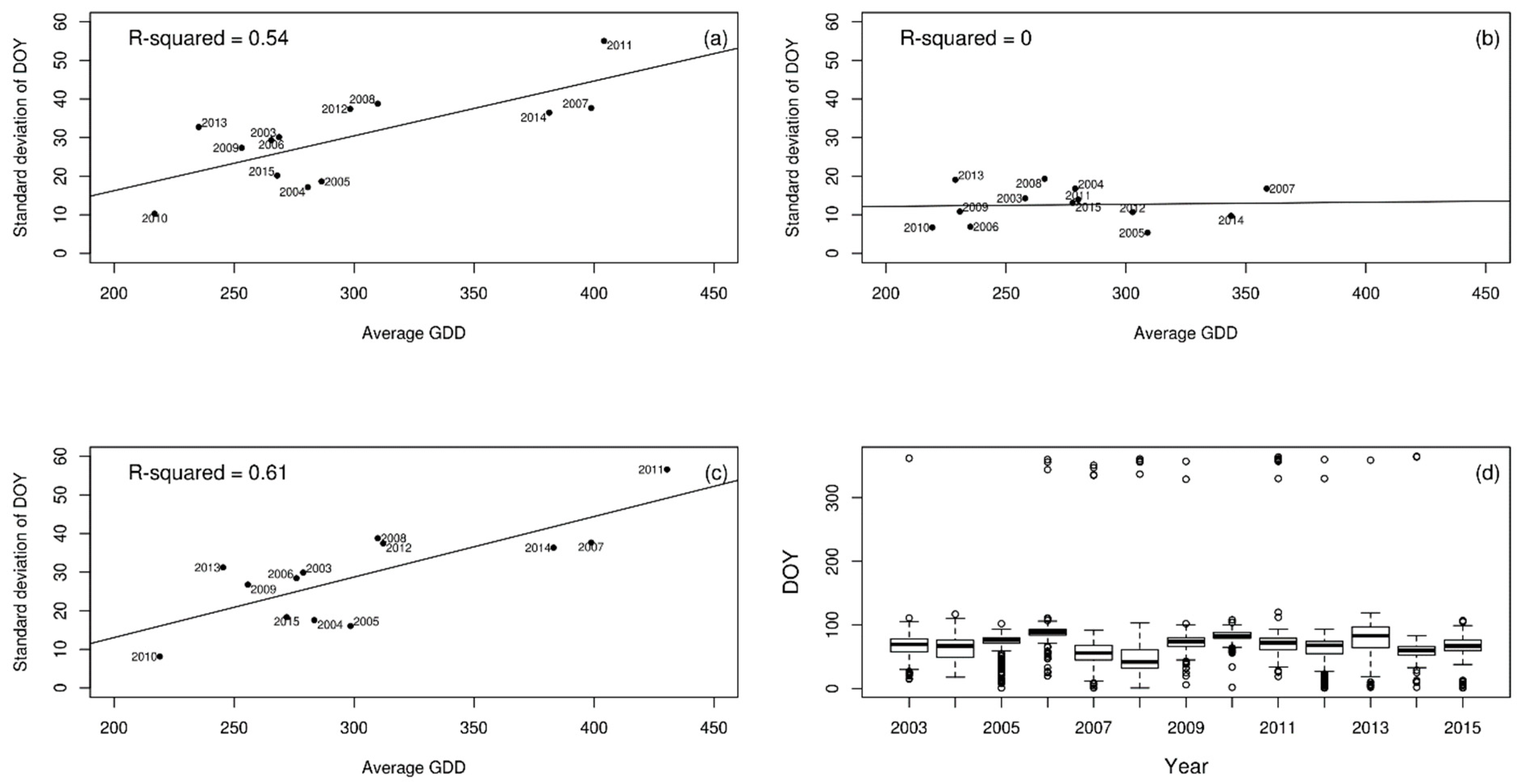
| Lesser celandine | 0.54 | 0.00 | 0.61 |
| Wood anemone | 0.43 | 0.28 | 0.40 |
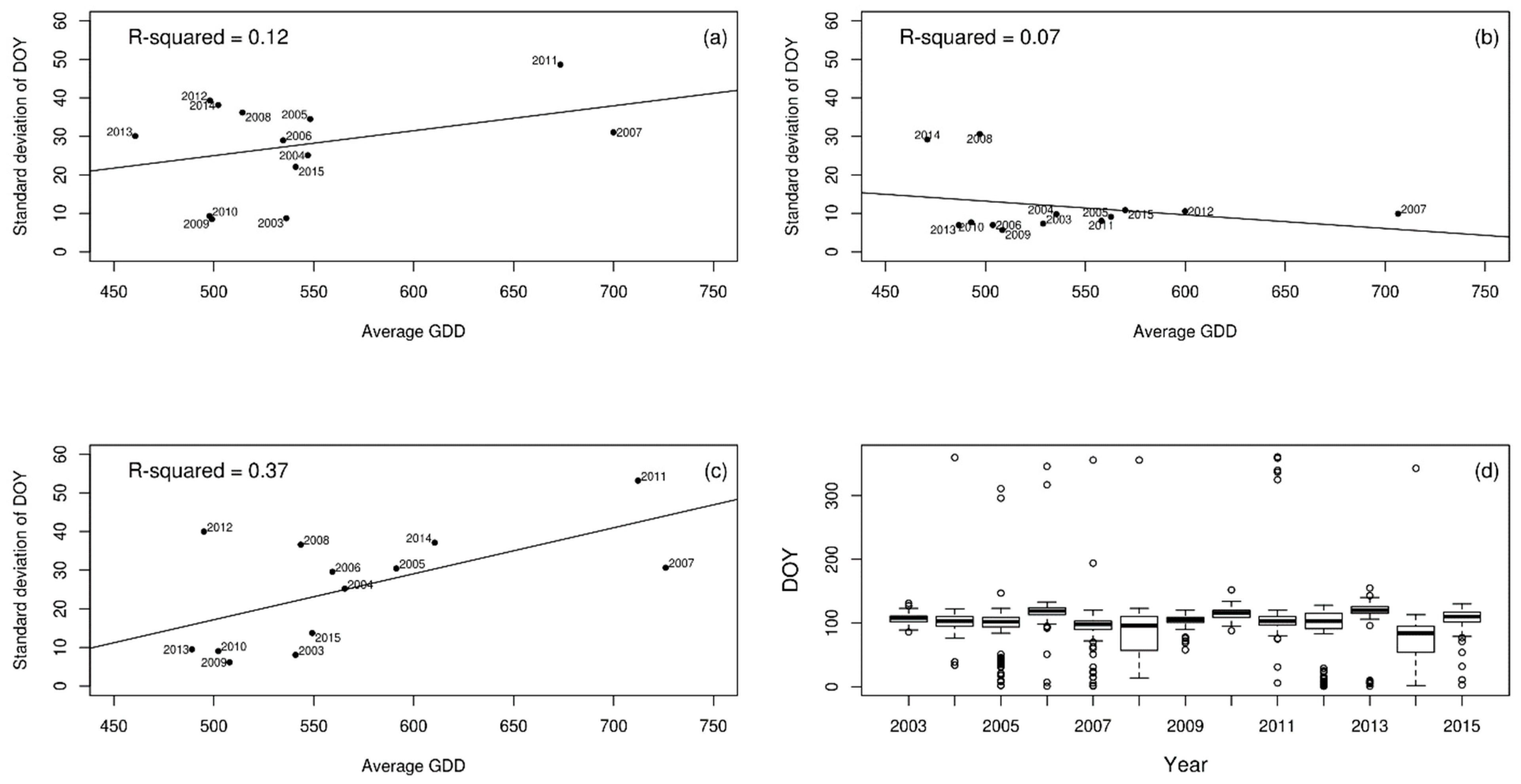
| Cow parsley | 0.12 | 0.07 | 0.37 |
| Pedunculate oak | 0.35 | 0.16 | 0.36 |
© 2018 by the authors. Licensee MDPI, Basel, Switzerland. This article is an open access article distributed under the terms and conditions of the Creative Commons Attribution (CC BY) license (http://creativecommons.org/licenses/by/4.0/).
Share and Cite
Mehdipoor, H.; Zurita-Milla, R.; Augustijn, E.-W.; Van Vliet, A.J.H. Checking the Consistency of Volunteered Phenological Observations While Analysing Their Synchrony. ISPRS Int. J. Geo-Inf. 2018, 7, 487. https://0-doi-org.brum.beds.ac.uk/10.3390/ijgi7120487
Mehdipoor H, Zurita-Milla R, Augustijn E-W, Van Vliet AJH. Checking the Consistency of Volunteered Phenological Observations While Analysing Their Synchrony. ISPRS International Journal of Geo-Information. 2018; 7(12):487. https://0-doi-org.brum.beds.ac.uk/10.3390/ijgi7120487
Chicago/Turabian StyleMehdipoor, Hamed, Raul Zurita-Milla, Ellen-Wien Augustijn, and Arnold J. H. Van Vliet. 2018. "Checking the Consistency of Volunteered Phenological Observations While Analysing Their Synchrony" ISPRS International Journal of Geo-Information 7, no. 12: 487. https://0-doi-org.brum.beds.ac.uk/10.3390/ijgi7120487