A New Approach to Line Simplification Based on Image Processing: A Case Study of Water Area Boundaries


School of Resource and Environmental Sciences, Wuhan University, Wuhan 430079, China
*
Author to whom correspondence should be addressed.
ISPRS Int. J. Geo-Inf. 2018, 7(2), 41; https://0-doi-org.brum.beds.ac.uk/10.3390/ijgi7020041
Submission received: 29 October 2017
/
Revised: 16 January 2018
/
Accepted: 28 January 2018
/
Published: 30 January 2018
Abstract
:Line simplification is an important component of map generalization. In recent years, algorithms for line simplification have been widely researched, and most of them are based on vector data. However, with the increasing development of computer vision, analysing and processing information from unstructured image data is both meaningful and challenging. Therefore, in this paper, we present a new line simplification approach based on image processing (BIP), which is specifically designed for raster data. First, the key corner points on a multi-scale image feature are detected and treated as candidate points. Then, to capture the essence of the shape within a given boundary using the fewest possible segments, the minimum-perimeter polygon (MPP) is calculated and the points of the MPP are defined as the approximate feature points. Finally, the points after simplification are selected from the candidate points by comparing the distances between the candidate points and the approximate feature points. An empirical example was used to test the applicability of the proposed method. The results showed that (1) when the key corner points are detected based on a multi-scale image feature, the local features of the line can be extracted and retained and the positional accuracy of the proposed method can be maintained well; and (2) by defining the visibility constraint of geographical features, this method is especially suitable for simplifying water areas as it is aligned with people’s visual habits.
1. Introduction
Line simplification is the process of reducing the complexity of line elements when they are expressed at a larger scale while maintaining their bending characteristics and essential shapes [1,2,3]. For decades, as the most important and abundant map elements, line elements have been an important area of research in cartography. Due to the complexity of the shape and diversity of line elements, it is difficult to design a perfect automated algorithm for line simplification. The line simplification algorithm is used to generate the graphical expression of a line at different scales, and three basic principles should be followed during simplification [4,5,6]: (1) maintaining the basic shape of curves, namely, the total similarity of graphs; (2) maintaining the accuracy of the characteristic points of bending; (3) maintaining the contrast of the curving degree in different locations.
Since the 1970s, classic algorithms used for line simplification have been proposed [7,8,9,10,11]. The Douglas–Peucker (DP) algorithm [8] uses a distance tolerance to subdivide the original line features in a recursive way. When the distance between the vertices and the line segment connecting the two original points is within a certain range, the vertices are eliminated. Li and Openshaw [9] presented a new approach to line simplification based on the natural process that people use to observe geographical objects. The method simulates the natural principle. The ratio of input and target resolutions is used to calculate the so-called “smallest visible object”. The method proved to be effective for detecting and retaining the overall shape of line features. Visvalingam and Whyatt [10] attempted to realize the progressive simplification of line features by using the concept of “effective area”. Based on the analysis and detection of line bends, Wang and Muller [11] proposed a typical algorithm for line simplification, which can generate reasonable results.
In recent years, research on line simplification has focused on shape maintenance [12,13,14,15,16], topological consistency [17,18], geo-characteristics [19,20,21,22], and data quality [23,24,25,26,27,28,29]. Jiang and Nakos [13] presented a new approach for line simplification based on shape detection of geographical objects in self-organizing maps. Dyken et al. [17] developed an approach for the simultaneous simplification of piecewise curves. The method uses the constrained Delaunay triangulation to preserve the topological relations between the linear features. Nabil Mustafa et al. [19] presented a method for line simplification based on the Voronoi diagram. First, the complex cartographic curve is divided into a series of safe sets. Then, the safe sets are simplified by using methods such as the DP algorithm. With this method, the intersections of the lines input can be avoided. Nöllenburg et al. [20] proposed a method for polylines morphing at different levels of detail. The method can be used to perform continuous generalization for linear geographical elements such as rivers and roads. Park and Yu [21] developed an approach for hybrid line simplification. In comparison with the single simplification algorithms, the method proved to be more effective in the field of vector displacement. Stanislawski et al. [23] studied various types of metric assessments such as the Hausdorff distance, segment length, vector displacement, areal displacement and sinuosity for the generalization of linear geographical elements. Their research can provide a reference for the appropriate parameter-settings of line generalization at different scales. Nakos et al. [24] made full use of the operations of data exaggeration, typification, enhancement, smoothing, or any combination thereof while performing line simplification. The study made remarkable progress regarding the highly automated generalization of full-life-circle data.
Other algorithms have been proposed for simplifying polygonal boundaries [30,31,32,33,34]. To reduce the area change, McMaster [30] presented a method for line simplification based on the integration of smoothing and simplification. Bose et al. [29] proposed an approach to simplifying polygonal boundaries. In their research, according to a given threshold of area change, the path that contains the smallest number of edges is used for simplification. Buchin et al. [32] presented an area-preserving method for the simplification of polygonal boundaries using an edge-move operation. During the process, the orientation of the polygons can be maintained by the edge-move operation that moves edges of the polygons inward or outward.
Studies of line representation based on image theory have mainly focused on polygonal approximation [35,36,37,38]. Kolesnikov and Fränti [36] presented a method for determining the optimal approximation of a closed curve. In the study, the best possible starting point can be selected by searching in the extended space of the closed curve. Ray and Ray [38] developed an approach for polygonal approximation based on a proposition of exponential averaging.
As indicated above, most studies have used vector data to simplify line elements or polygonal boundaries, but few studies have used raster data. In addition, the existing studies based on image theory cannot meet the requirements of cartographic generalization because of a lack of consideration of the three basic principles. However, with the continuous development of computer vision and artificial intelligence technology, extracting and processing information from a growing number of unstructured datasets (such as pictures, street view, 3D models, video and so on) is a worthwhile and challenging task. Thus, line simplification based on image data is necessary due to the growing number of unstructured datasets.
Therefore, this paper presents a new line simplification method based on image processing techniques using unstructured image data. Following this introduction, Section 2 describes a comparison between scale space and map generalization, which lays out a theoretical foundation for line simplification based on image data. In Section 3, we describe the methods of line simplification, which include corner detection, minimum-perimeter polygons and matching candidate points and approximate feature points. Section 4 presents the results of experiments that illustrate the proposed approaches, and a discussion and analysis of our approaches are provided. Section 5 presents our conclusions.
2. Scale Space and Map Generalization
Scale space describes a theory of signal representation at different scales [39]. In the process of the scaling transformation, the representation of images at different scales is parametrized according to the size of the smoothing kernel, and the fine-scale details can be successively suppressed [40]. As the primary type of scale space, the linear scale space is widely applicable and has the effective property of being able to be derived from a small set of scale space axioms. The Gaussian kernel and its derivatives are regarded as the only possible smoothing kernels [41].
For a given image , the linear Gaussian scale-space representation can be described as a family of derived signals , which is defined by the convolution of the image with the two-dimensional Gaussian kernel [41]:
such that
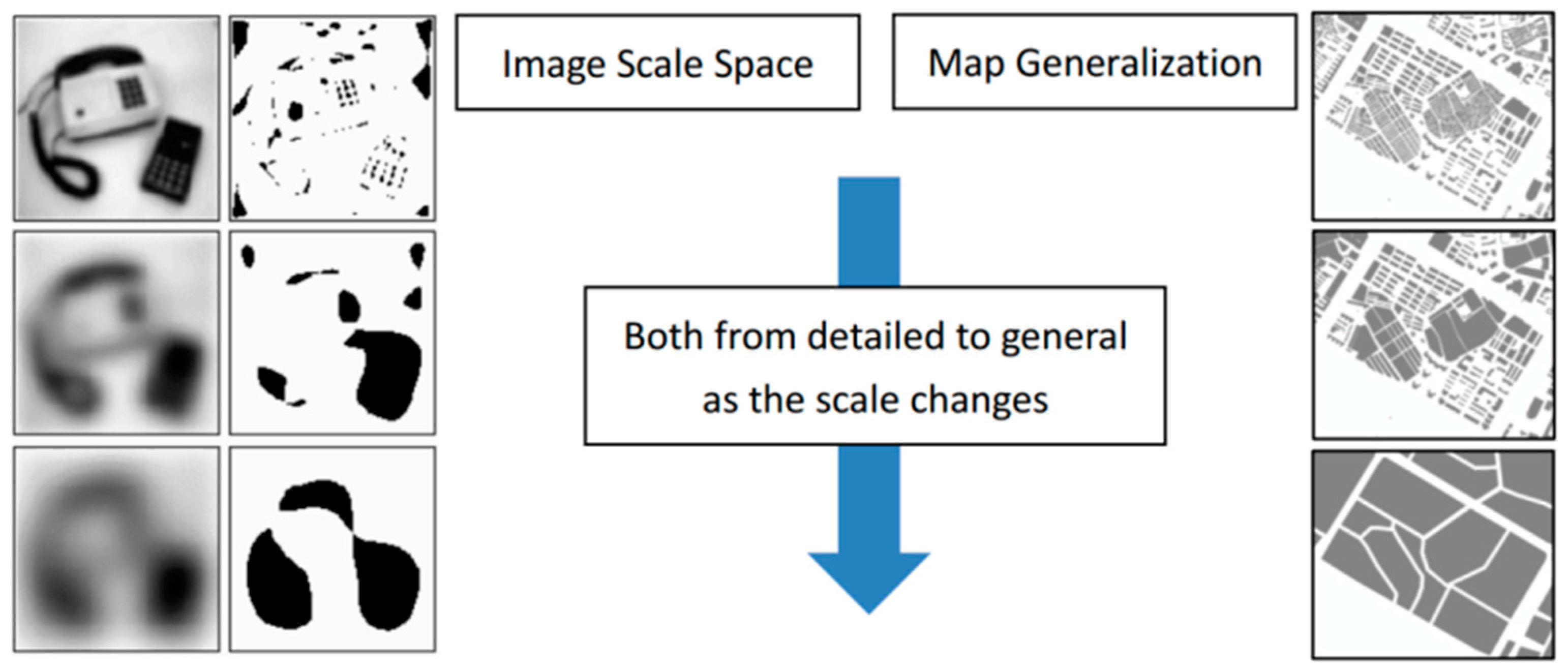
In Equation (1), denotes the two-dimensional Gaussian filter, x denotes the distance from the origin in the horizontal axis, y denotes the distance from the origin in the vertical axis, and t denotes the standard deviation of the Gaussian distribution. In Equation (2), the semicolon in the argument of L indicates that the convolution is executed only over the variables x and y. The scale variate t after the semicolon indicates which scale level is being defined. Although a continuum of scales can be described by the definition of L, only a finite, discrete set of levels will be taken into account in the representation of scale space. The variance of the Gaussian filter is described by the scale parameter . When the scale parameter , the filter g is an impulse function such that , which indicates that the scale-space representation at scale level becomes the image f itself. With an increase of the scale parameter t, the filter g becomes increasingly larger. As L is the outcome of smoothing f with a filter, an increasing number of details from the images will be removed in this process. Since describes the standard deviation of the filter, the details of an image that are significantly smaller than this value will be removed at scale level t. In Figure 1, the left panel shows a typical example of a scale space representation at different scales.
Analogously, cartographic generalization, or map generalization, is a process that simplifies the representation of geographical data to generate a map at a smaller scale from a larger scale map [42]. For example, the right panel of Figure 1 represents residential areas at different scales. In this process, the details are abandoned and the general information is retained. As the essence of both processes is the same, this paper seeks to use rasterize map data and image processing methods based on the scale space theory to simplify the polygonal boundary on a map.
3. Methodologies for Line Simplification
We use the image processing techniques such as corner detection and calculation of the minimum-perimeter polygon to simplify the polygonal boundary. The methods for simplifying lines can be divided into three steps: (1) corner detection based on scale space to extract the local features of the objects from the raster data and ensure the positioning accuracy of feature points; (2) calculation of a minimum-perimeter polygon (MPP) to simplify the overall shape of the objects; and (3) matching candidate points and approximate feature points from the MPP. The detailed steps are as follows.
3.1. Classification and Detection of Corners
Typically, a point with two different and dominant edge directions in the local neighbourhood of this point can be considered a corner. The corners in images represent critical information in local image regions and describe local features of objects. A corner can be a point with locally maximal curvature on a curve, a line end, or a separate point with local intensity minimum or maximum. The detection of corners can be successfully applied to many applications, such as object recognition, image matching or motion tracking [43,44,45]. As a result, there have been a number of studies on different approaches for corner detection [46,47,48,49,50]. As shown in Figure 2, corners can be divided into three types: acute and right corners, round corners, and obtuse corners. Figure 2d shows the curvature plot of a round corner in Figure 2b.
In 1992, Rattarangsi and Chin presented a multi-scale approach for corner detection of planar curves based on curvature scale space (CSS) [51]. The method is based on Gaussian scale space, which is made up of the maxima of the absolute curvature of the boundary function presented at multiple scales. Because the method based on CSS performs well in maintaining invariant geometric features of the curves at different scales, Mokhtarian and Suomela developed two algorithms of corner detection based on CSS [52,53] for greyscale images. These methods based on CSS are effective for corner detection and are robust to noise. In this study, we developed an improved method of corner detection for polygonal boundaries. The definition of curvature K, from [54], is as follows:
where , , , , and represents the convolution operator, while represents a Gaussian distribution of width , is the first derivative of and is the second derivative of .
In traditional single-scale methods, such as references [46,48], the corners are detected by considering their local characteristics. In these cases, the fine features could be missed, and some noise may be incorrectly interpreted as corners. The benefit of the CSS algorithms is that they take full advantage of global and local curvature characteristics, and they balance the influence of both types of characteristics in the process of extracting corners. To better extract the local features of the polygonal boundary from the images and ensure the positioning accuracy of feature points, we add the classification stage of corner points on the basis of CSS, and an improved method of corner detection based on CSS is proposed as follows:
- (1)
- To obtain the binary edges, the method of Canny edge detection [55] is applied.
- (2)
- Edge contours are extracted from the edge map as described in the CSS method.
- (3)
- After the edge contours are extracted, the curvature of each contour is computed at a small scale to obtain the true corners. If the absolute curvature of a point is the local maximum, it can be treated as a corner candidate.
- (4)
- Classification of corner points. According to the mean curvature within a region of support, an adaptive threshold is calculated. The round corner is marked by comparing the adaptive threshold with the curvature of corner candidates. According to a dynamically recalculated region of support, the angles of the corner candidates should also be calculated, and any false corners will be eliminated. As a result, the corners can be divided into three types: acute and right corners, round corners, and obtuse corners.
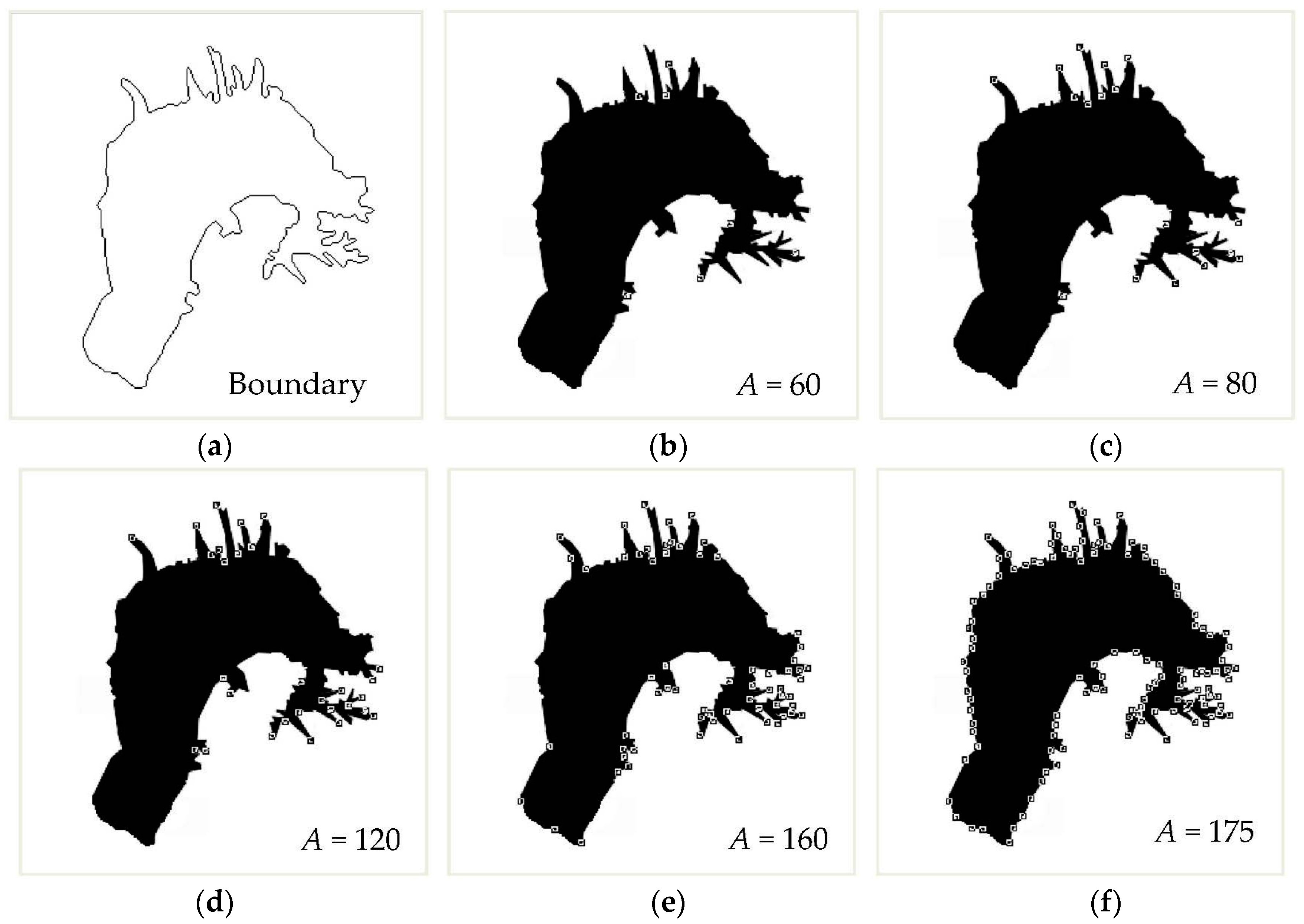
Figure 3 shows the results of corner detection with different angles. As shown in Figure 3, increasing the angle generates more corner points.
There are three important parameters in the proposed method based on CSS: (1) Ratio (R): R is used to detect round corners, and it represents the minimum ratio of the major axis to the minor axis of an ellipse; (2) Angle (A): A is used to detect the acute, right and obtuse angle corners, and it represents the maximum angle used when screening for corners; (3) Filter (F): F represents the standard deviation of the Gaussian filter during the process of computing curvature. In Figure 3, the default values are F = 3 and R = 1. Detailed information about the adaptive threshold and the parameter R can be found in reference [55].
3.2. Calculation of a Minimum-Perimeter Polygon
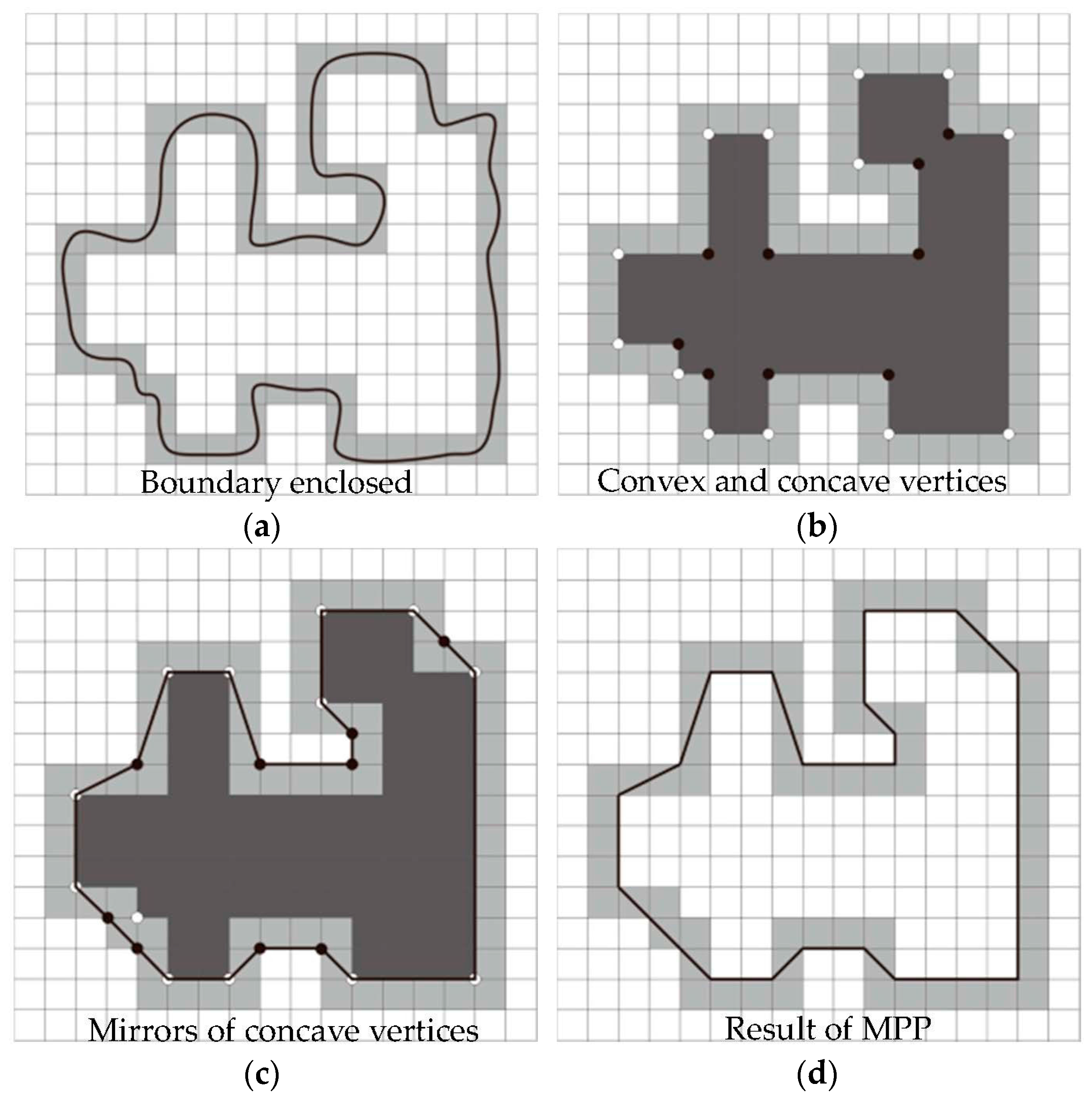
For a given boundary, the aim of the approximation is to obtain the essence of the shape, and there should be as few segments as possible. This problem deserves attention in general, and polygonal approximation methods of modest complexity are well suited to image-processing tasks. Among a variety of technologies, a minimum-perimeter polygon (MPP) [56] is one of the most powerful methods to represent a boundary. The following discussion gives the basic definitions of a MPP [57].
An MPP of a boundary represents a rasterized polygon with the shortest perimeter among all the polygons whose images coincide with the given boundary. To intuitively generate an algorithm to calculate MPPs, an appealing approach is to enclose a boundary with a set of concatenated cells, as shown in Figure 4a. The boundary can be treated as a rubber band that is allowed to shrink. The rubber band will be limited by the inner and outer walls of the bounding region defined by the cells, as shown in Figure 4b,c. Finally, the shape of a polygon with the minimum perimeter is created by shrinking the boundary, as shown in Figure 4d. All the vertices of the polygon are produced with the corners of either the inner or the outer wall of the grey region. For a given application, the goal is to use the largest possible cell size to produce MPPs with the fewest vertices. The detailed process of finding these MPP vertices is as follows.
The cellular method just described reduces the shape of the original polygon, which is enclosed by the original boundary, to the area circumscribed by the grey wall, as shown in Figure 4a. This shape in dark grey is presented in Figure 4b, and its boundary is made up of four connected straight-line segments. Assuming that the boundary is traversed in a counter-clockwise direction, when a turning point appears in the traversal, it will be either a convex or a concave vertex, and the angle of a turning point is an interior angle of the 4-connected boundary. Figure 4b shows the convex and concave vertices with white and black dots, respectively. We see that each black (concave) vertex in the dark grey region corresponds to a mirror vertex in the light grey region, which is located diagonally opposite the black vertex. The mirrors of all the concave vertices are presented in Figure 4c. The vertices of the MPP consist of convex vertices in the inner wall (white dots) and the mirrors of the concave vertices (black dots) in the outer wall.
The accuracy of the polygonal approximation is determined by the size of the cells (cellsize). For example, if , then the size of one cell is . If , then the size of one cell is . In a limited case, when the size of each cell equals a pixel in the boundary, the error between the MPP approximation and the original boundary in each cell would be at most s, where s represents the minimum possible distance between pixels. If each cell in the polygonal approximation is forced to be centred on its corresponding pixels in the original boundary, the error can be reduced by half. The detailed algorithm to find the vertices of the MPP can be found in reference [57].
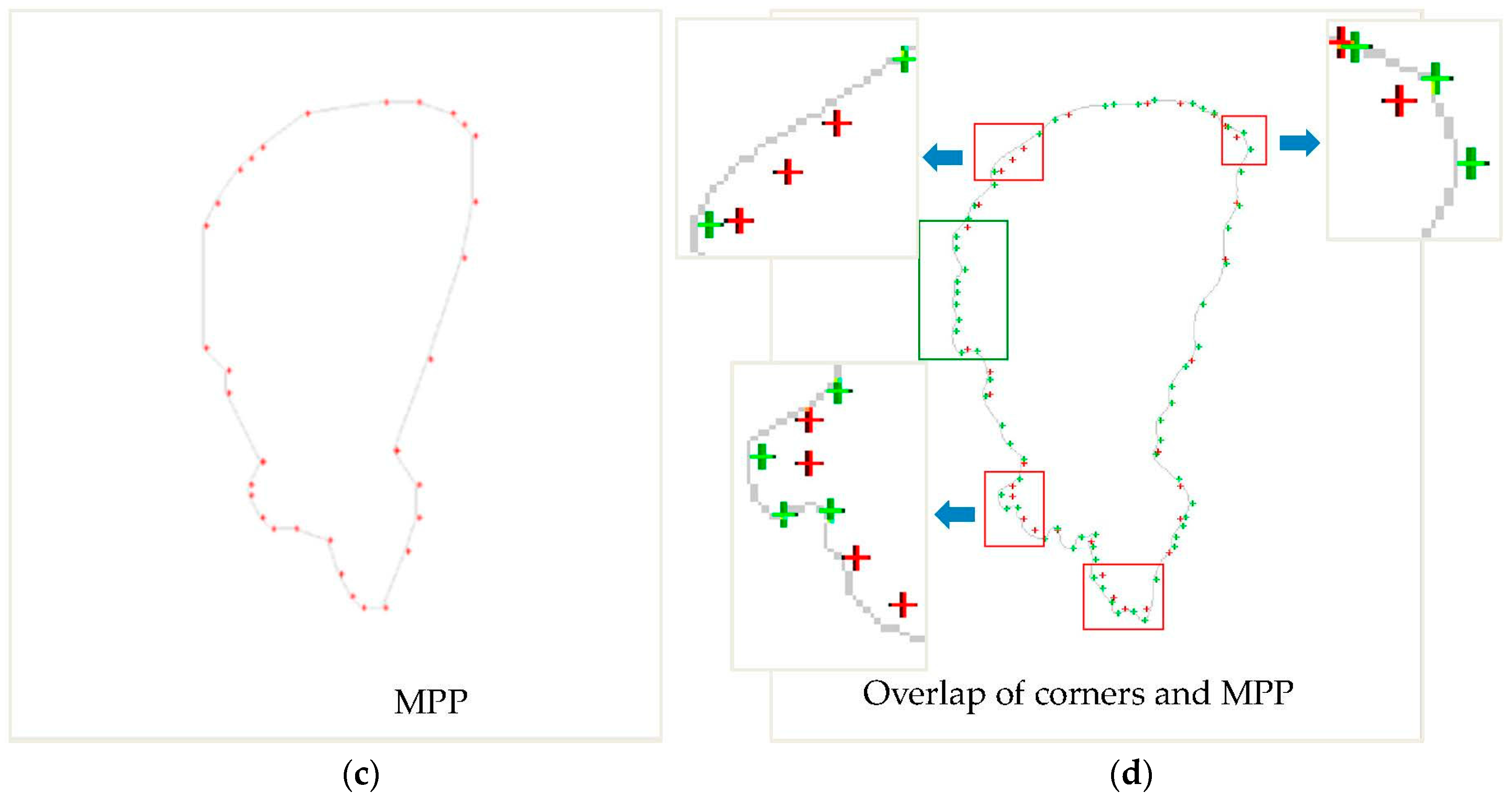
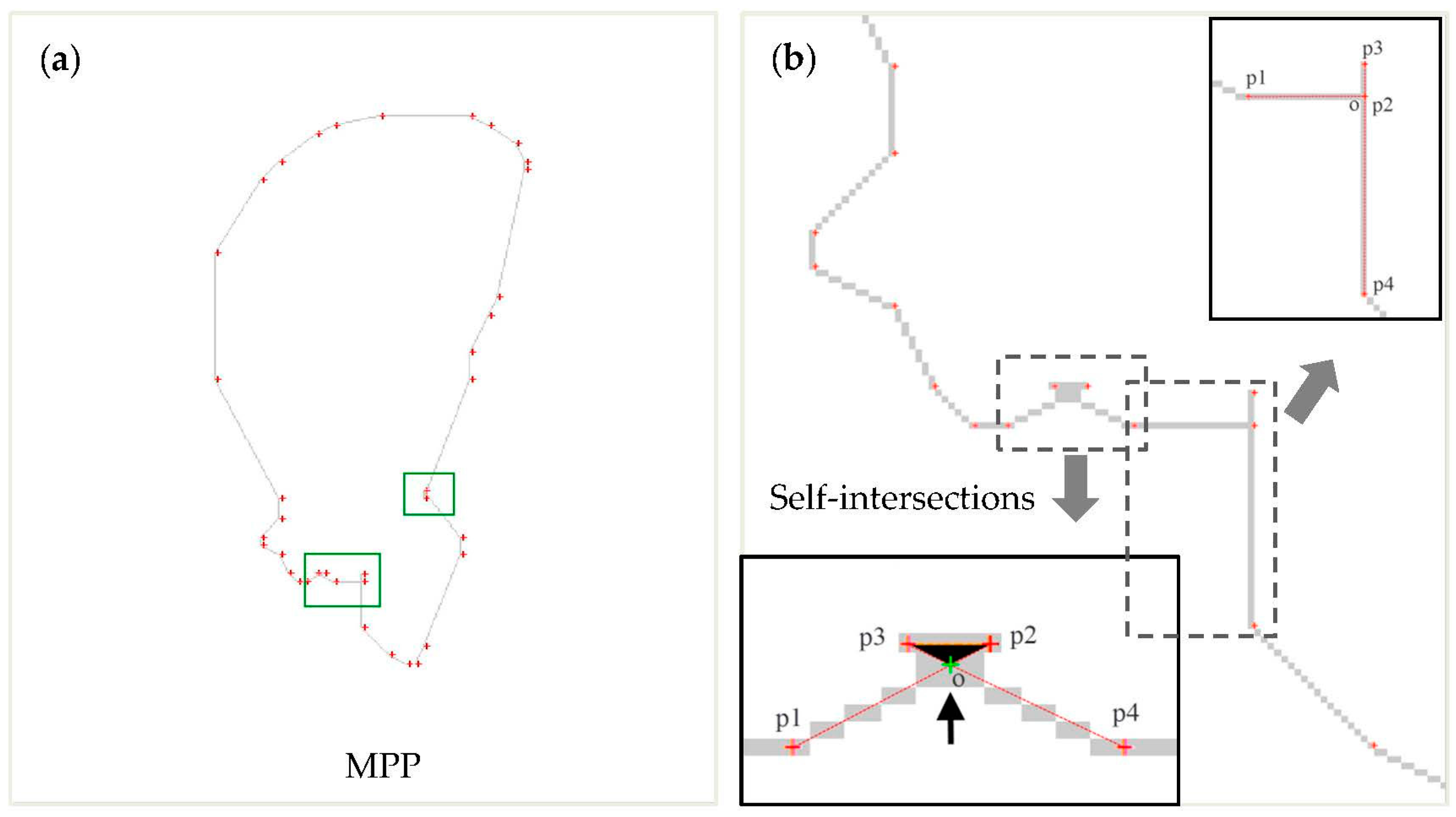
Figure 5 shows typical examples. Figure 5a shows the result of boundary extraction. Figure 5b shows the result of corner detection. Figure 5c shows the minimum-perimeter polygon of the lake when cellsize = 6. Figure 5d shows the overlapping result between corner points (marked with green) and MPP points (marked with red). As we can see from Figure 5d, the MPP points are mostly not on the boundary, as shown in the red box. Furthermore, when the boundary is relatively flat, the distribution of MPP points is sparse, as shown in the green box. Although the MPP algorithm has a certain ability to simplify the overall shape of a polygon, it obviously cannot meet the requirements of cartographic generalization because of the uneven distribution and location error of points. Conversely, although the corner points have good localization accuracy and show local characteristics, they cannot meet the requirements of cartographic generalization because of the lack of overall shape simplification. Therefore, in the following sections, we will take full advantage of these two methods to simplify the polygonal boundary.
3.3. Simplification of a Polygonal Boundary
To simplify the overall shape of the lake and ensure the localization accuracy of local feature points, we combine the advantages of two algorithms and use the method of matching neighbouring points. The main steps are shown below.
(1) Remove the self-intersecting lines of MPP
When the parameter cell size changes, it can easily produce self-intersecting lines in narrow zones, as shown in Figure 6a. Normally, the cross section is not visible because the cell size is too big. As shown in Figure 6b, the line segment composed of points p1, p2, p3, and p4 is self-intersecting. The cross section op3p2 is not visible and should be removed. Thus, point p3 and p2 will be removed, and the intersection point o will be added to constitute a new polygon. In some instances, point p2 and o are overlapping, as shown in the upper right of Figure 6b.
(2) Filter corner points
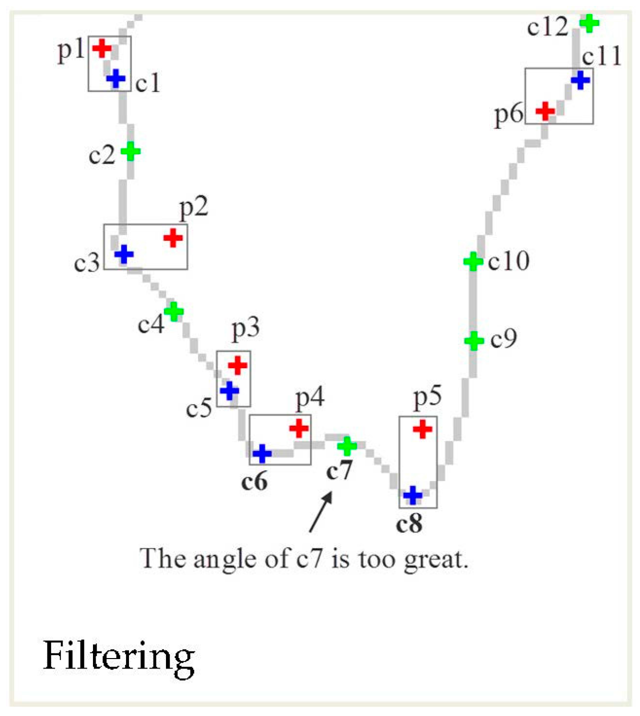
The simplified feature points will be selected from corner points that are in the neighbourhood of the MPP points after the removal of self-intersections. If the distance between the corner point and the MPP point is the shortest, the corner point will be selected. As shown in Figure 7, the red points are the MPP points after the removal of self-intersections, the green points are the corner points, and the blue points are the selected corner points that make up the simplified point set. However, it may contain multiple corner points with similar distances to the MPP point in the neighbourhood of the MPP points. Given that the features of a sharp area are more obvious than those of at flat area, the corner with a small angle in a neighbourhood of MPP points will be selected preferentially. For example, points c6 and c7 are both in the neighbourhood of point p4, and the distance between c6 and p4 is close to the distance between c7 and p4. In this case, the simplified point set will be selected according to the types of corner points. The priority of corner points for selection is as follows: point of acute (right) angle > point of rounded angle > point of obtuse angle.
In Figure 7, the angle of point c6 is smaller than the angle of point c7, so point c6 is selected.
(3) Densification of simplified points
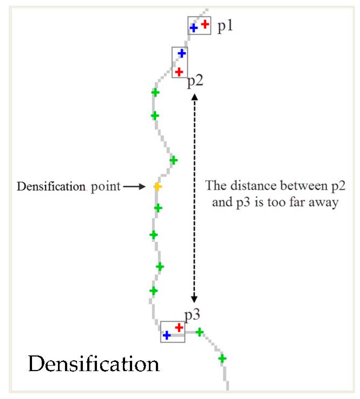
When the boundary is relatively flat, the distribution of MPP points is sparse, as shown in Figure 8. In this case, because the distance between two adjacent points is too great, to maintain the consistency of the distribution density of the points, the corner point in the neighbourhood of the midpoint of the connecting line between the two adjacent points should be selected as the densification point. The yellow point in Figure 8 is the densification point. If there are several candidate corner points in the neighbourhood of the midpoint, the point should be selected according to the priority outlined in the second step.
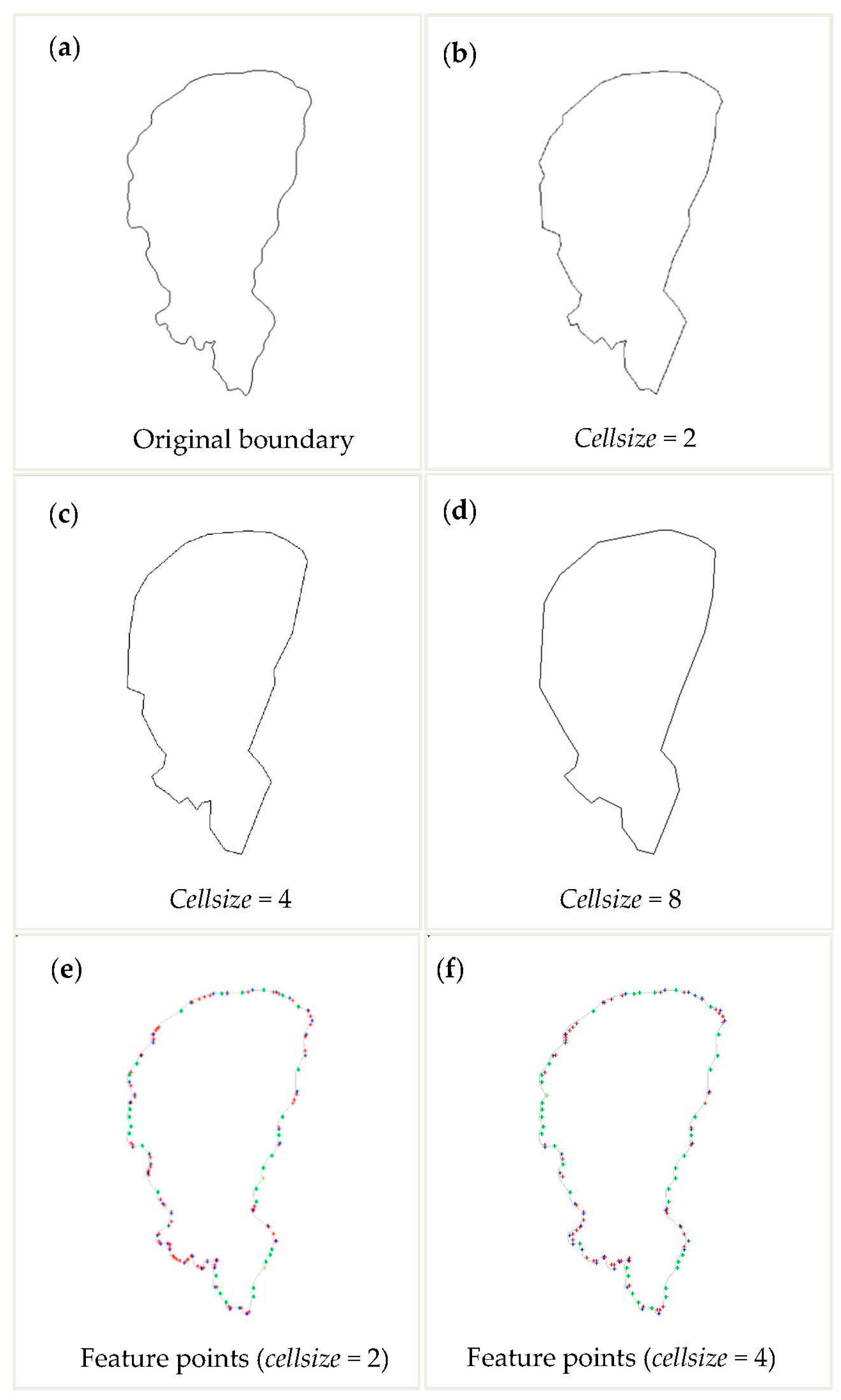
Figure 9 shows an example of simplifying a polygonal boundary using the method proposed in this paper. Figure 9a shows the original boundary of a lake. The number of pixels comprising the original boundary is 959. Figure 9b–d show the simplification results of the lake when cellsize = 2, cellsize = 4 and cellsize = 8, respectively. Cellsize is the side length (pixel) of square cells. As shown in the figures, with increasing cellsize, more details of the boundary are abandoned. The overall shape of the boundary is simplified as well, and the simplified points have good localization accuracy. Figure 9e,f show the calculation results of different types of feature points when cellsize = 2 and cellsize = 4. The red points are the MPP points after the removal of self-intersections, the green points are the corner points, the blue points are the selected corner points that make up the simplified point set, and the yellow points are the densification points. With increasing cellsize, the MPP points after the removal of self-intersections decrease in number.
Table 1 shows detailed information on parameter changes before and after simplification. With increasing cellsize, the numbers of MPP points and simplified points decrease in number, and the percent changes in length increase. The percent changes in area are relatively small.
4. Experiments and Evaluations
4.1. Study Area
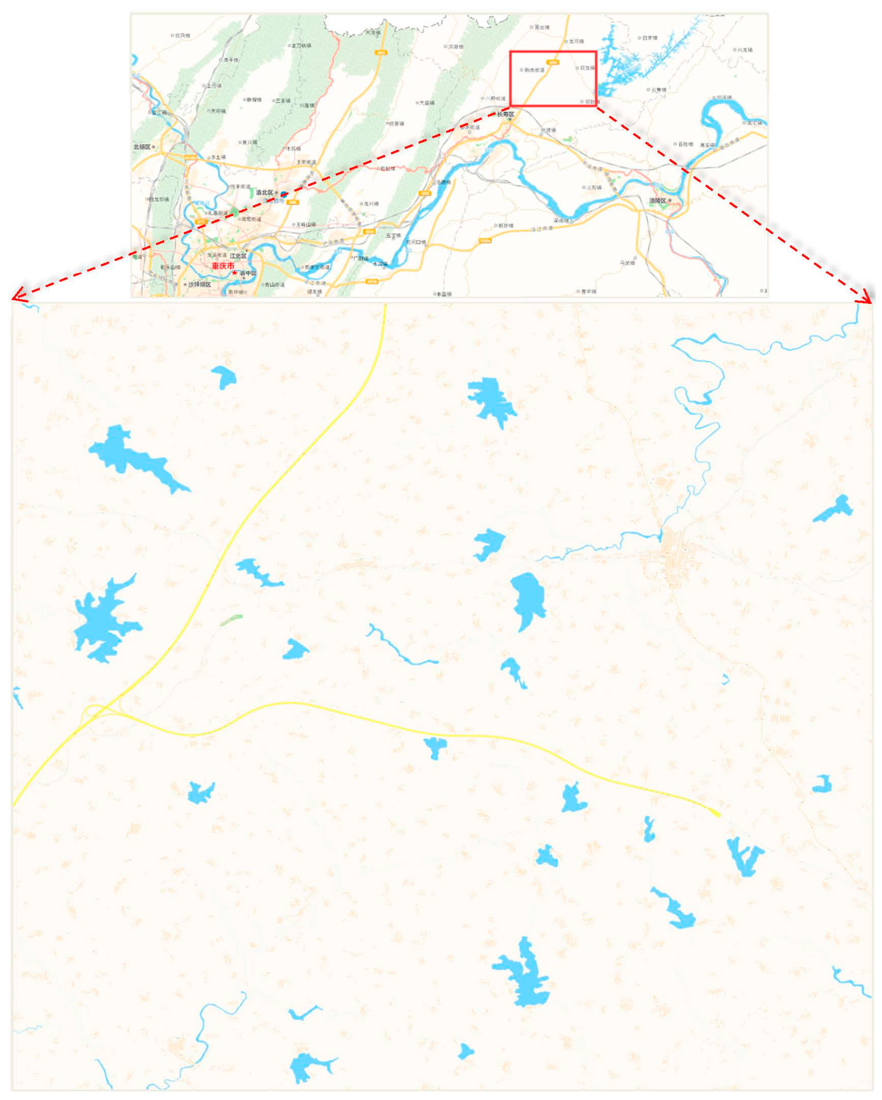
In this study, experimental data that were used to simplify water areas at a large scale were obtained from the Tiandi map for China. We used data at the 17th level from the Tiandi map. The corresponding scale at the 17th level is 1:5000. The study area is located in the northeast part of Changshou District of Chongqing in China, as shown in Figure 10. Several lakes and a few rivers are present within this area. The study area is located between 29.90 and 29.99 degrees north latitude and between 107.12 and 107.23 degrees east longitude. The data at the 17th level consist of 4480 tiles, and the size of one tile is 256 by 256 pixels (1 pixel = 1.194 m). The coordinate range of these tiles is 43,700 ≤ x ≤ 43,769, 209,082 ≤ y ≤ 209,145. The image that is formed from these tiles contains 17,920 by 16,384 pixels.
4.2. Results and Analysis
There are many difficulties when extracting water areas from the tile map. As the data are obtained from the Tile Map Server (TMS) on the Internet, each tile has a uniform resource locator (URL), which can be downloaded for free. Compared with the other geographic elements on a map, the water areas are usually rendered in blue. Thus, we can use a method of threshold segmentation to separate the water areas from the other geographical elements on a map. However, because of overlays with other geographical elements, such as annotations and roads, the extracted water areas from a map may contain obvious “holes” or fractures. Considering these two factors, there are three steps for extracting water areas from a tile map: (1) extracting water areas by colour segmentation; (2) connecting fractures in water areas; and (3) filling holes in water areas. The detailed explanations and demonstrations can be found in a previous work [58].
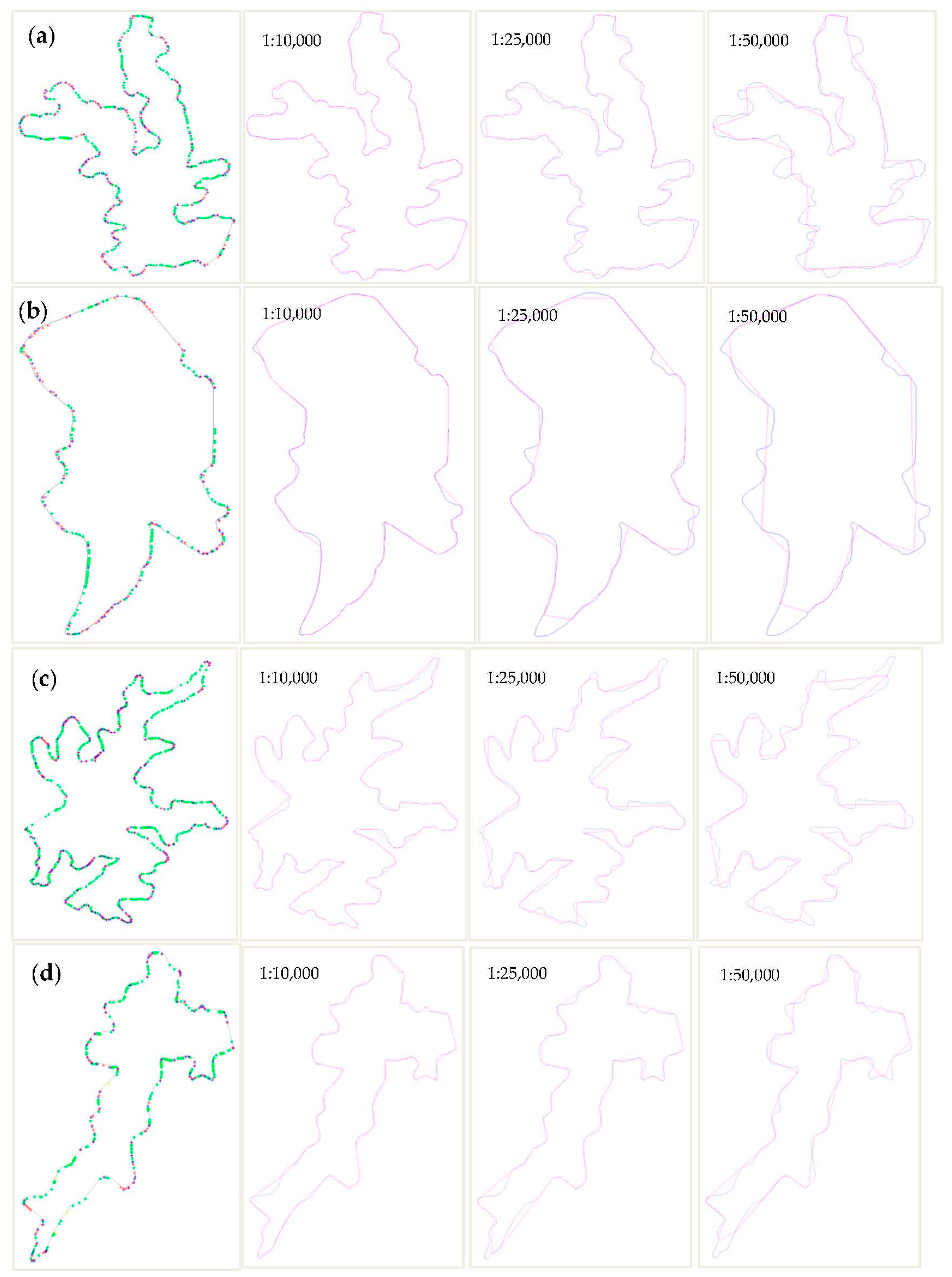
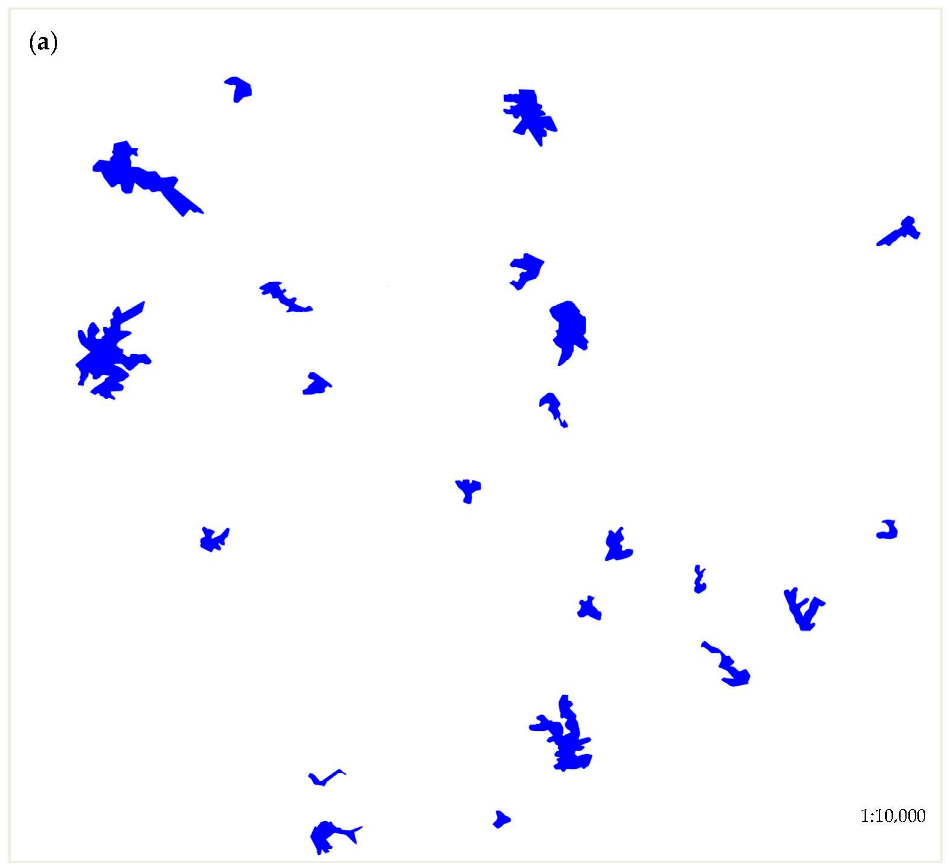
Figure 11 shows the experimental data after extraction. We removed the narrow rivers and retained the lakes. There were 22 lakes in total. We chose four lakes, as marked with red boxes in Figure 11, to display in detail. Figure 12 shows the results of simplification of the four lakes at different scales (1:10,000, 1:25,000, 1:50,000). In Figure 12(a1,b1,c1,d1) show the calculation results of different types of feature points when cellsize = 10. The red points are the MPP points after the removal of self-intersections, the green points are the corner points, the blue points are the selected corner points that make up the simplified point set, and the yellow points are the densification points.
As shown in Figure 12, with an increase in cellsize, the simplifying effect of the boundary becomes more obvious. In the process of increasing the cellsize, small bends are gradually abandoned. As for overall characteristics, the shape of the whole lake is maintained after simplification. As for local characteristics, the most prominent feature points in the local area are maintained, and the position precision of the feature points is guaranteed. The number of all points before and after simplification is shown in Table 2.
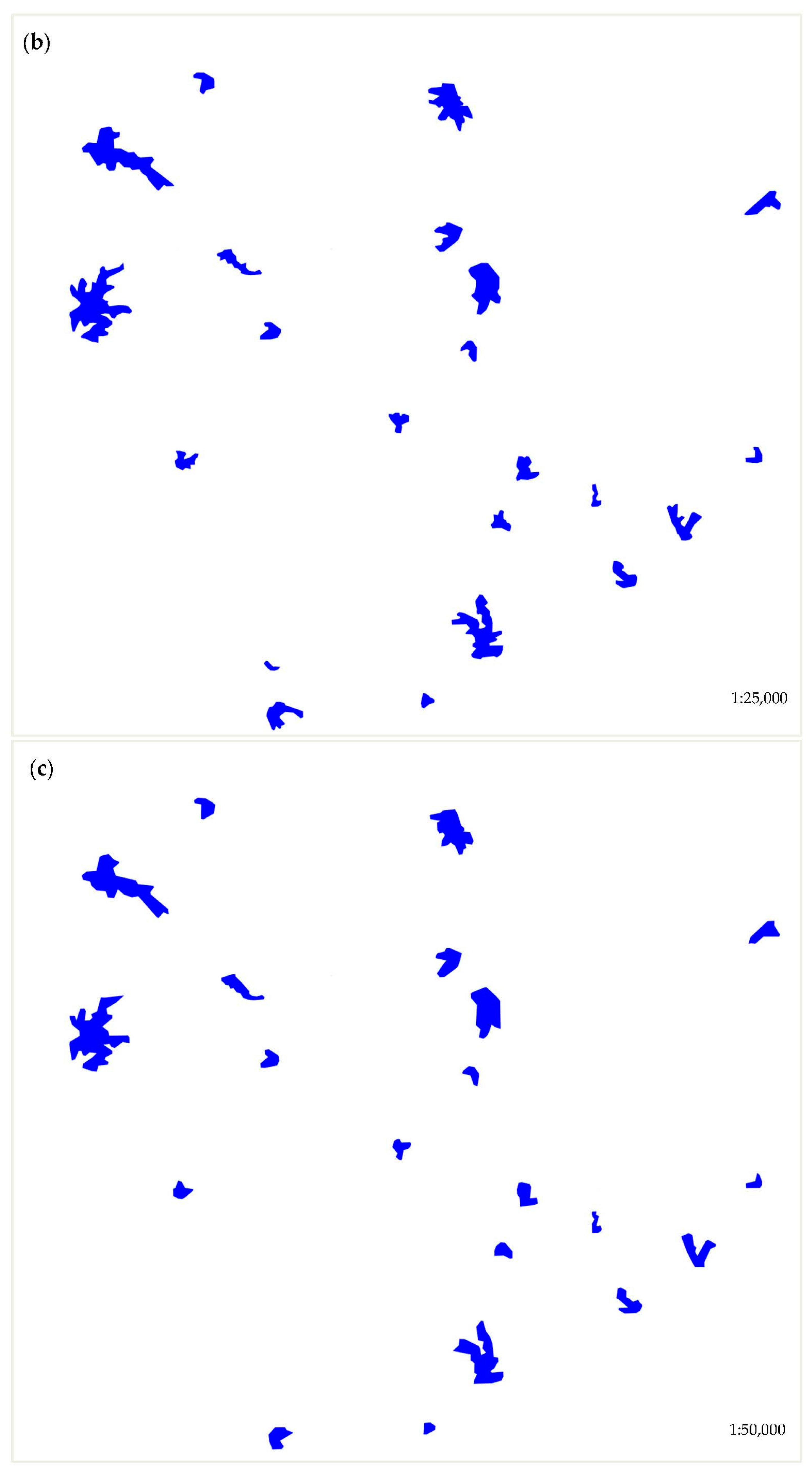
As shown in Table 2, with an increase in cellsize, the number of simplified points decreases. Figure 13 shows the results of simplification of all the lakes at three different scales (1:10,000, 1:25,000, 1:50,000). The values of the cellsize are cellsize = 10, cellsize = 30, cellsize = 50, respectively. To obtain a good result, the default values of R, A and F can be set as R = 1.5, A = 175, and F = 3, respectively. We also used the DP and Wang and Muller [11] (WM) algorithms to conduct contrastive experiments. During the experiment, the original water areas are raster data. We use ArcGIS software (www.arcgis.com) for the conversion of the data format and registration of the scale. Given that the three methods are controlled by different parameters, it is difficult to strictly determine whether their results reflect the same map scale. By combining the rules for setting values from reference [1] and manual experience in cartographic generalization, the parameters of the DP and WM algorithms used in this study can be set as shown in Figure 4, which is relatively reasonable in this experiment.
Muller proposed that v = 0.4 mm [59] (size on the drawing) is the minimum value when it is visually identifiable. Thus, we define the minimum visibility (mv) of a feature as follows:
To ensure the best visual effect, we set the parameter value mv to be approximately 1 during the experiment. The corresponding relationship of scale, cellsize, and mv is shown in Table 3:
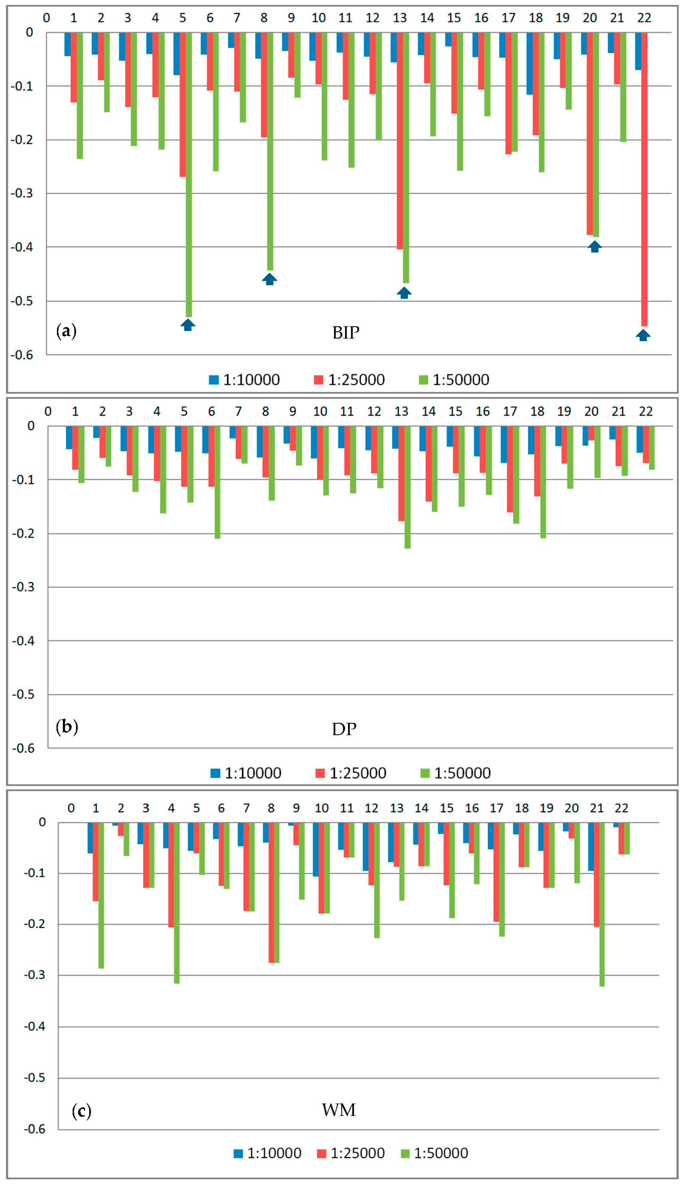
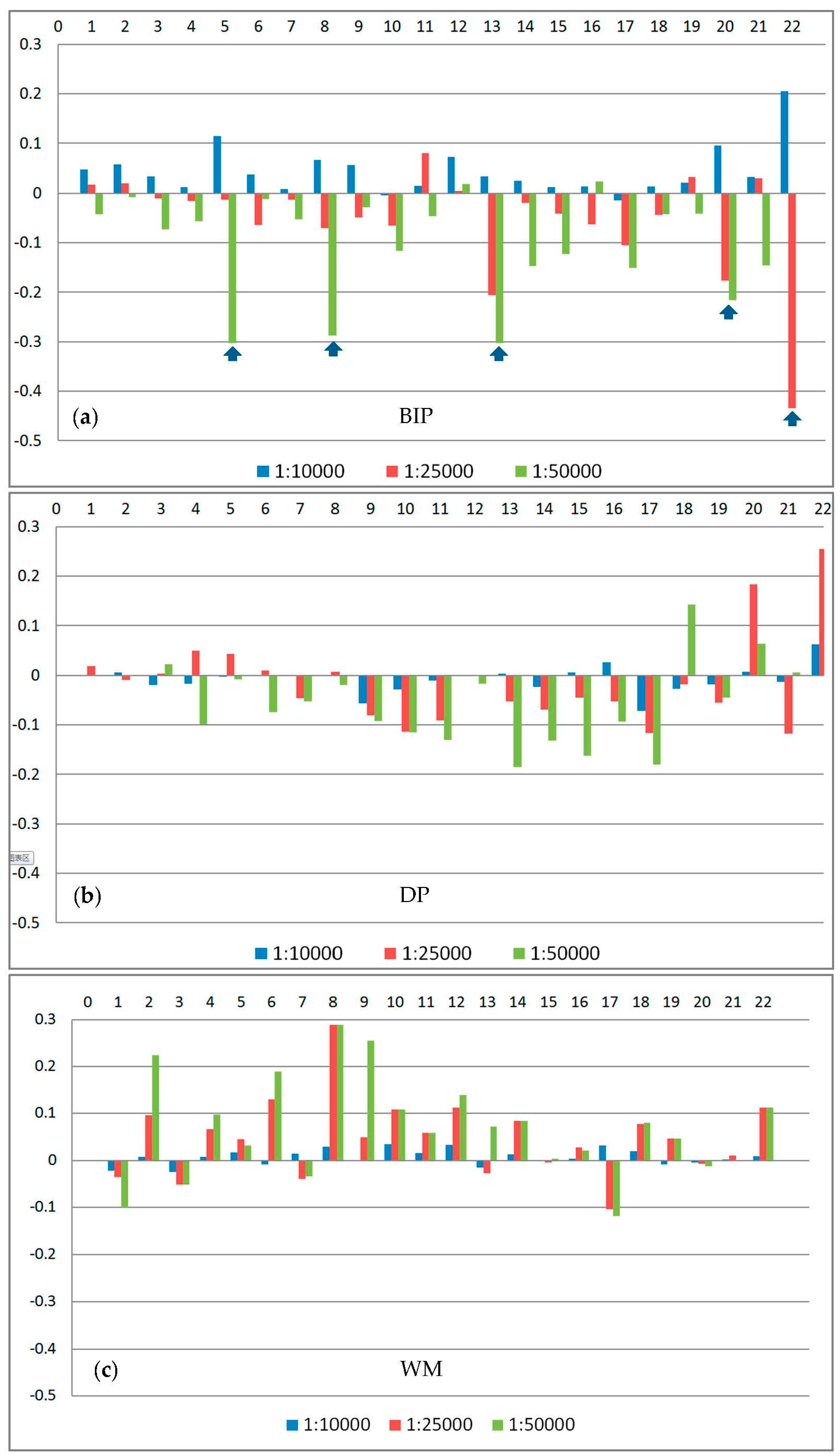
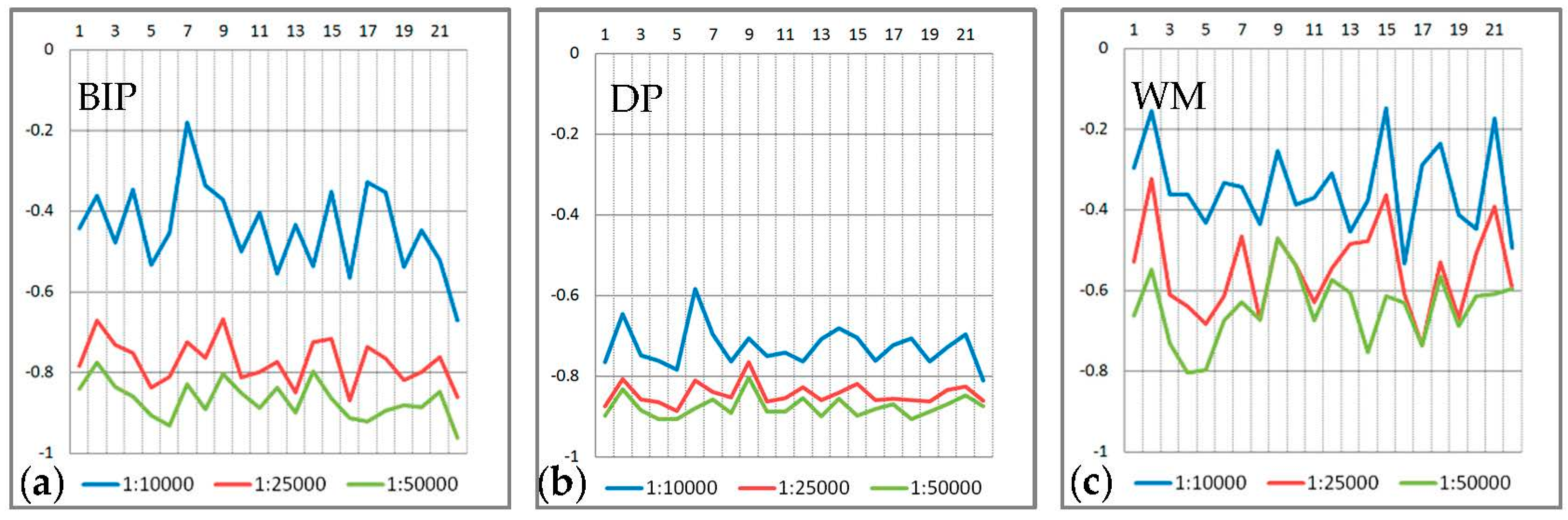
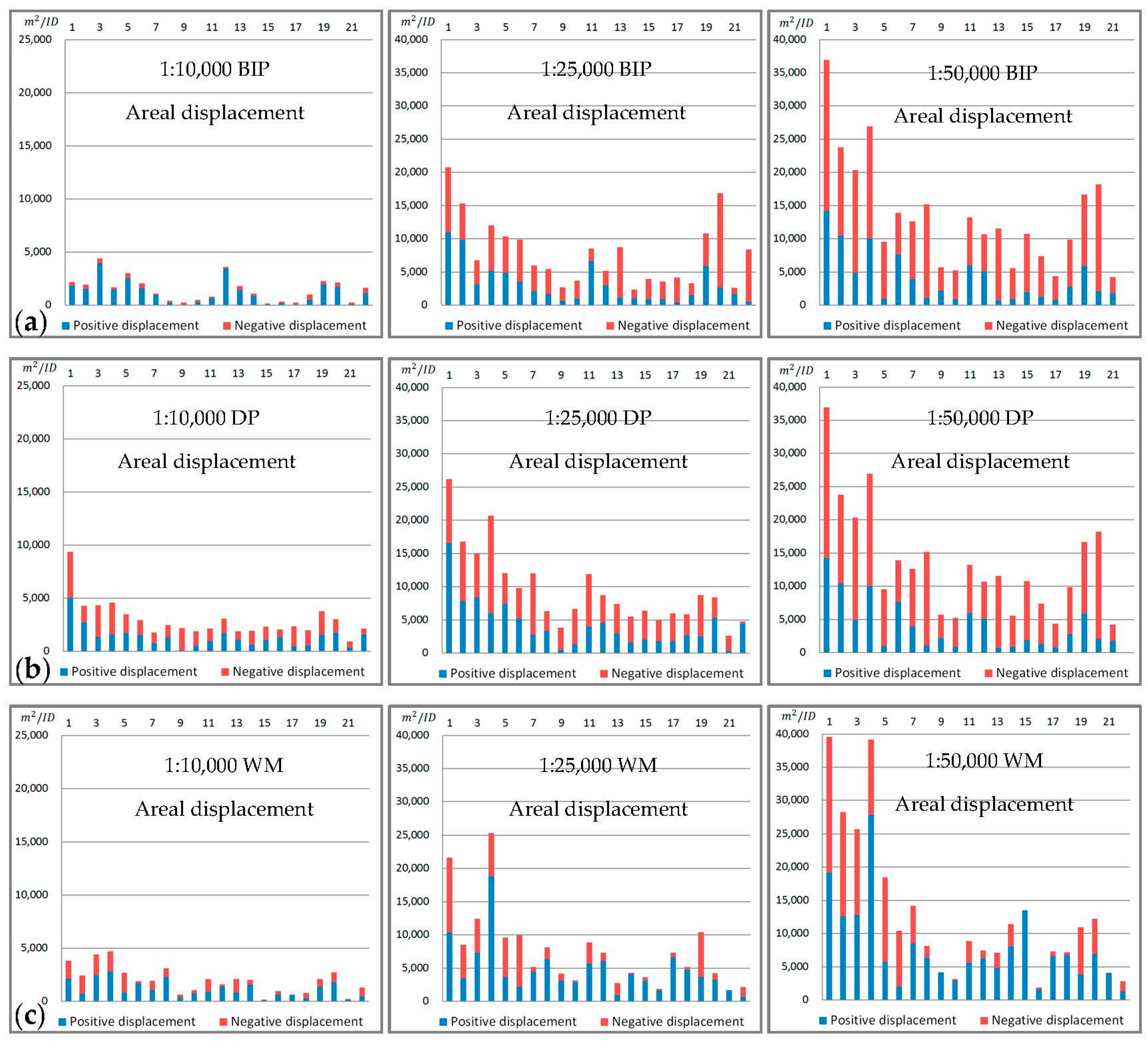
Table 4 presents the comparisons of three groups of experiments. Figure 13 shows the simplification results for all the lakes in three different scales. The values of the parameter cellsize at three scales are cellsize = 10, cellsize = 30, cellsize = 50, respectively. Figure 14 shows the typical simplification results of the DP, WM, and BIP methods. Figure 15, Figure 16 and Figure 17 show the comparison of changes in length, area and number of points at the three scales for the three methods, respectively. Figure 18 and Table 5 show the comparison of areal displacement at the three scales for the three methods.
From Figure 13, Figure 14, Figure 15, Figure 16, Figure 17 and Figure 18 and Table 4 and Table 5, we observe the following:
- (1)
- The proposed BIP method can be effectively used for polygonal boundary simplification of water areas at different scales. The BIP method for the simplification of water areas aligns with people’s visual processes. With an increase in visual distance, i.e., as the scale becomes smaller, the small parts of an object will appear invisible. The invisible parts should be abandoned in the process of simplification. As shown in Figure 14, the black polygons are the results of simplification using the DP and WM algorithms, and the pink polygons are the results of simplification using the proposed BIP method. The smaller part of the polygon marked with the black dotted box can be removed using our method because this part is too small to be seen when the scale is small. The same areas are conserved using the DP and WM algorithms, and this type of simplification is unreasonable as we can hardly see these areas at the small scale.
- (2)
- The changes in length resulting from the proposed BIP method are slightly larger than those resulting from the DP and WM methods. With a decrease in scale, the changes in length increase for the three methods. As shown in Table 4, the average per cent changes in the perimeters at scales 1:25,000 and 1:50,000 are −0.176 and −0.253, respectively, for the BIP method. The corresponding per cent changes for the DP method are −0.094 and −0.133, respectively. However, there is an interesting phenomenon in Figure 15, which shows the detailed changes in the perimeter of each object at three scales. As shown in Figure 15, five lakes have remarkable changes in their perimeters because of characteristics based on the visual processes of the BIP method, as described in the above Section 2. In other words, removing the invisible parts leads to significant changes in the perimeters. The changes in the area between the original and simplified boundaries follow the same rule, as shown in Figure 16.
- (3)
- Figure 17 shows the comparison of changes in the number of points. The average per cent change in the number of points of the proposed method is −0.442 at the largest scale. With an increase in cellsize, the per cent change increases. The average per cent change in the number of points is −0.869 at the smallest scale. Overall, the point reduction ratio of the proposed method at the three scales is lower than the DP method, but higher than the WM methods. Additionally, as shown in Table 4, since the BIP method uses the image data to perform simplification, the execution time of the proposed method is longer than the other two methods.
- (4)
- We also use the areal displacement [60] to measure the location accuracy. As shown in Figure 18 and Table 5, the average areal displacement of the BIP method at the three scales is smaller than that of the DP method. In addition, the average areal displacement of the BIP method at scales of 1:10,000 (1494 m2) is smaller than that of the WM method (1974 m2). However, the average areal displacement of the BIP method at scales of 1:25,000 and 1:50,000 (7918 m2 and 13,468 m2, respectively) is larger than that of the WM method (7628 m2 and 13,362 m2, respectively). Thus, the location accuracy of the proposed method at the three scales is better than that of the DP method, but close to the WM method.
4.3. A Case of Hierarchical Simplification Using the BIP Method
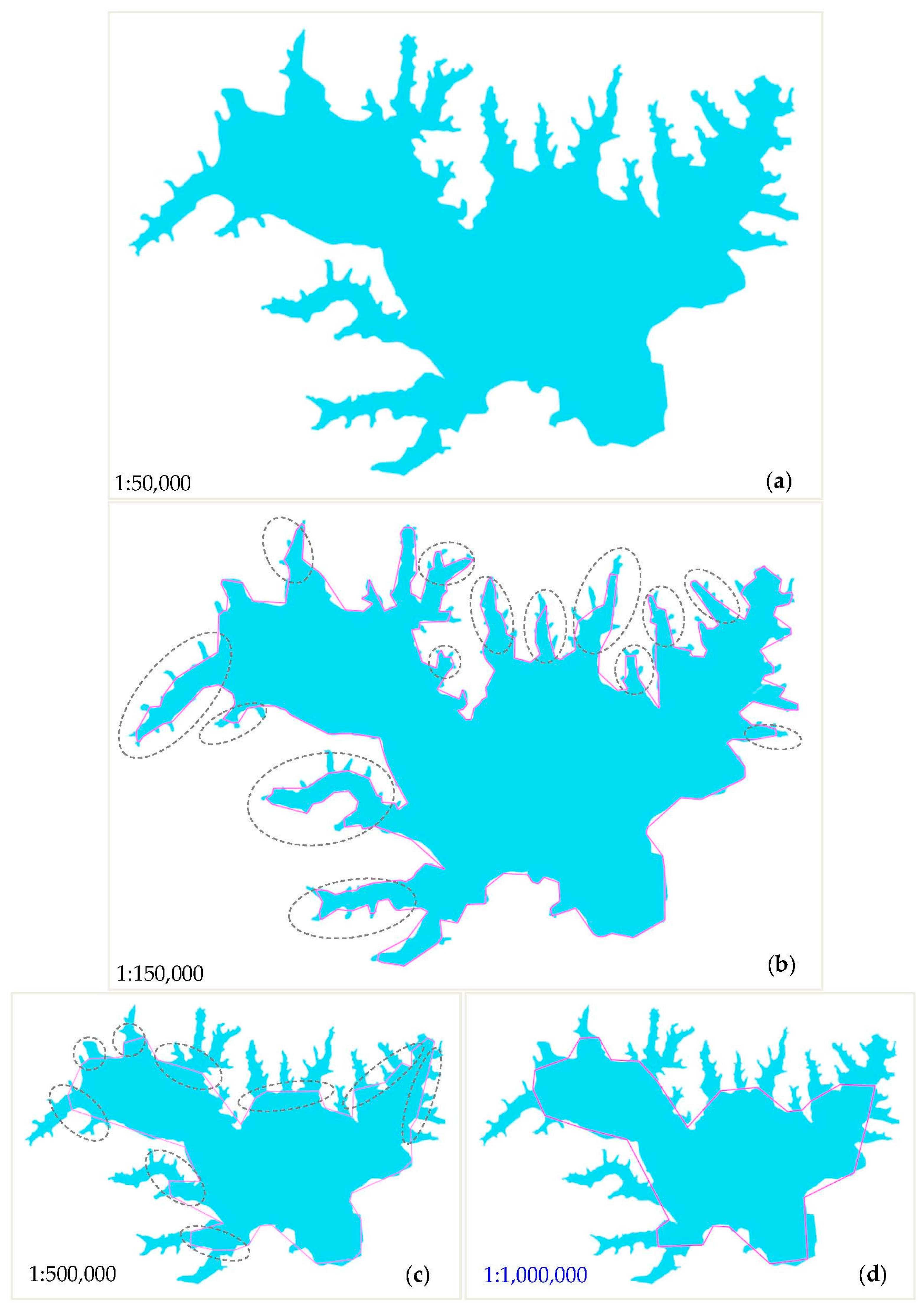
As the proposed BIP method aligns with people’s visual processes, it is very applicable to the simplification of water areas with hierarchical branches. Figure 19 shows the case of hierarchical simplification using the BIP method. Figure 19a is the original lake with detailed branch information. The experimental data that were used to simplify water areas at a small scale were obtained from the Baidu map of China. We used data at the 14th level from the Baidu map. The corresponding scale at the 14th level is 1:50,000. The original resolution of the lake is 1 pixel = 16 m. Figure 19b shows the simplification results after removing the branches in the first layer using the BIP method. Some typical simplification areas are marked with grey dotted ovals. As cellsize increases, the thicker branches will be removed. Figure 19c shows the simplification results after removing the branches in the second layer using the BIP method. According to the definition of the visibility constraint, the values cellsize = 9, cellsize = 33 and cellsize = 60 are used to generate the results at the scales of 1:150,000, 1:500,000, and 1:1,000,000, respectively.
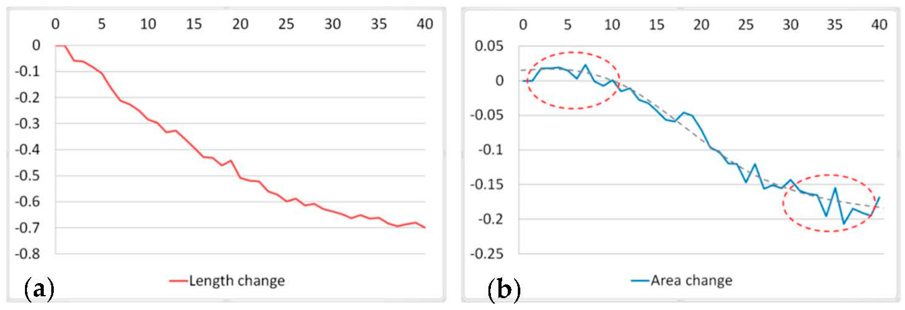
Figure 20 shows the changes in length (Figure 20a) and area (Figure 20b) with increasing cellsize. The default values of R, A and F are R = 1.5, A = 175, and F = 3, respectively. As shown in Figure 20a, the rate of change in length is relatively uniform when the cellsize is less than 30. When the cellsize is greater than 30, the rate of change begins to decrease. As shown in Figure 20b, the rate of change in area is relatively high when the cellsize is in the range of 10–30, but relatively gradual when the cellsize is in the ranges of 0–10 and 30–40. The values of the cellsize used for cutting off the branches are located within the gradual range. These values are cellsize = 9 (first layer) and cellsize = 33 (second layer).
5. Conclusions
This paper proposes a new approach for line simplification using image processing techniques based on a raster map. In the traditional methods of line simplification, vector data are used as the primary experimental data. However, our study focuses on the rules of people’s visual processes to simplify a water area boundary using the BIP method based on image data. The following conclusions can be drawn:
- (1)
- The proposed BIP method can be effectively used for polygonal boundary simplification of water areas at different scales. By using the method of corner detection based on CSS, the local features of the water areas are maintained.
- (2)
- The proposed BIP simplification method aligns with people’s visual processes. As long narrow parts (as shown in Figure 14a) usually attach around water areas, the BIP method can remove the invisible long, narrow parts when the scale decreases by the definition of the minimum visibility (mv) of a feature. Therefore, this method is especially suitable for simplifying the boundary of water areas at larger scales.
- (3)
- In comparison with the DP and WM methods, the length and area change of the proposed method is slightly larger at three scales, and the maximum average percentage difference of length at the three scales is only 0.06%, and the maximum average percentage difference of area at the three scales is only 0.05%. The location accuracy resulting from the proposed BIP method is better than that form the DP method, but close to the WM method.
- (4)
- Given that the proposed BIP method can more accurately remove the details that humans do not need at larger scales, the point reduction ratio of the proposed BIP method at the three scales is lower than the DP method, but higher than the WM method. Additionally, since the BIP method uses the image data to perform simplification, the execution time of the BIP method is longer than the other two methods.
In addition to water areas, we tried to apply the proposed BIP method to any other line elements such as contour lines, buildings, or administrative boundaries. Apparently, due to the different characteristics of different types of line elements, the method cannot satisfy the needs of data generalization for all types of line elements, such as buildings with orthogonal characteristics. In the future, the proposed method should be improved and applied to other geographic line elements.
Acknowledgments
This research was supported by the National Key Research and Development Program of China (Grant No. 2017YFB0503500), the National High-Tech Research and Development Plan of China (Grant No. 2015AA1239012), and the National Natural Science Foundation of China (Grant No. 41531180).
Author Contributions
Yilang Shen and Tinghua Ai conceived and designed the study; Yilang Shen performed the experiments; Yilang Shen analyzed the results and wrote the paper; Yilang Shen, Tinghua Ai and Yakun He read and approved the manusctipt.
Conflicts of Interest
The authors declare no conflict of interest.
References
- Ai, T.; Ke, S.; Yang, M.; Li, J. Envelope generation and simplification of polylines using Delaunay triangulation. Int. J. Geogr. Inf. Sci. 2017, 31, 297–319. [Google Scholar] [CrossRef]
- Ratschek, H.; Rokne, J.; Leriger, M. Robustness in GIS algorithm implementation with application to line simplification. Int. J. Geogr. Inf. Sci. 2001, 15, 707–720. [Google Scholar] [CrossRef]
- Mitropoulos, V.; Xydia, A.; Nakos, B.; Vescoukis, V. The Use of Epsilon-convex Area for Attributing Bends along A Cartographic Line. In Proceedings of the 22nd International Cartographic Conference, La Coruña, Spain, 9–16 July 2005. [Google Scholar]
- Qian, H.; Zhang, M.; Wu, F. A new simplification approach based on the Oblique-Dividing-Curve method for contour lines. ISPRS Int. J. Geo-Inf. 2016, 5, 153. [Google Scholar] [CrossRef]
- Ai, T. The drainage network extraction from contour lines for contour line generalization. ISPRS J. Photogramm. Remote Sens. 2007, 62, 93–103. [Google Scholar] [CrossRef]
- Ai, T.; Zhou, Q.; Zhang, X.; Huang, Y.; Zhou, M. A simplification of ria coastline with geomorphologic characteristics reserved. Mar. Geodesy 2014, 37, 167–186. [Google Scholar] [CrossRef]
- Lang, T. Rules for the robot draughtsmen. Geogr. Mag. 1969, 42, 50–51. [Google Scholar]
- Douglas, D.H.; Peucker, T.K. Algorithms for the reduction of the number of points required to represent a digitized line or its caricature. Can. Cartogr. 1973, 10, 112–122. [Google Scholar] [CrossRef]
- Li, Z.L.; Openshaw, S. Algorithms for automated line generalization based on a natural principle of objective generalization. Int. J. Geogr. Inf. Syst. 1992, 6, 373–389. [Google Scholar] [CrossRef]
- Visvalingam, M.; Whyatt, J.D. Line generalization by repeated elimination of points. Cartogr. J. 1993, 30, 46–51. [Google Scholar] [CrossRef]
- Wang, Z.; Muller, J.C. Line generalization based on analysis of shape characteristics. Cartogr. Geogr. Inf. Sci. 1998, 25, 3–15. [Google Scholar] [CrossRef]
- Jiang, B.; Nakos, B. Line Simplification Using Self-organizing Maps. In Proceedings of the ISPRS Workshop on Spatial Analysis and Decision Making, Hong Kong, China, 3–5 December 2003. [Google Scholar]
- Zhou, S.; Jones, C. Shape-aware Line Generalisation with Weighted Effective Area. In Developments in Spatial Data Handling; Springer: Berlin, Germany, 2004; pp. 369–380. [Google Scholar]
- Raposo, P. Scale-specific automated line simplification by vertex clustering on a hexagonal tessellation. Cartogr. Geogr. Inf. Sci. 2013, 40, 427–443. [Google Scholar] [CrossRef]
- Gökgöz, T.; Sen, A.; Memduhoglu, A.; Hacar, M. A new algorithm for cartographic simplification of streams and lakes using deviation angles and error bands. ISPRS Int. J. Geo-Inf. 2015, 4, 2185–2204. [Google Scholar] [CrossRef]
- Samsonov, T.E.; Yakimova, O.P. Shape-adaptive geometric simplification of heterogeneous line datasets. Int. J. Geogr. Inf. Sci. 2017, 31, 1485–1520. [Google Scholar] [CrossRef]
- Dyken, C.; Dæhlen, M.; Sevaldrud, T. Simultaneous curve simplification. J. Geogr. Syst. 2009, 11, 273–289. [Google Scholar] [CrossRef]
- Saalfeld, A. Topologically consistent line simplification with the Douglas-Peucker algorithm. Cartogr. Geogr. Inf. Sci. 1999, 26, 7–18. [Google Scholar] [CrossRef]
- Mustafa, N.; Krishnan, S.; Varadhan, G.; Venkatasubramanian, S. Dynamic simplification and visualization of large maps. Int. J. Geogr. Inf. Sci. 2006, 20, 273–320. [Google Scholar] [CrossRef]
- Nöllenburg, M.; Merrick, D.; Wolff, A.; Benkert, M. Morphing polylines: A step towards continuous generalization. Comput. Environ. Urban Syst. 2008, 32, 248–260. [Google Scholar] [CrossRef]
- Park, W.; Yu, K. Generalization of Digital Topographic Map Using Hybrid Line Simplification. In Proceedings of the ASPRS 2010 Annual Conference, San Diego, CA, USA, 26–30 April 2010. [Google Scholar]
- Ai, T.; Zhang, X. The Aggregation of Urban Building Clusters Based on the Skeleton Partitioning of Gap Space. In The European Information Society: Leading the Way with Geo-Information; Springer: Berlin/Heidelberg, Germany, 2007; pp. 153–170. [Google Scholar]
- Stanislawski, L.V.; Raposo, P.; Howard, M.; Buttenfield, B.P. Automated Metric Assessment of Line Simplification in Humid Landscapes. In Proceedings of the AutoCarto 2012, Columbus, OH, USA, 16–18 September 2012. [Google Scholar]
- Nakos, B.; Gaffuri, J.; Mustière, S. A Transition from Simplification to Generalisation of Natural Occurring Lines. In Proceedings of the 11th ICA Workshop on Generalisation and Multiple Representation, Montpelier, France, 20–21 June 2008. [Google Scholar]
- Mustière, S. An Algorithm for Legibility Evaluation of Symbolized Lines. In Proceedings of the 4th InterCarto Conference, Barnaul, Russia, 1–4 July 1998; pp. 43–47. [Google Scholar]
- De Bruin, S. Modelling positional uncertainty of line features by accounting for stochastic deviations from straight line segments. Trans. GIS 2008, 12, 165–177. [Google Scholar] [CrossRef]
- Veregin, H. Quantifying positional error induced by line simplification. Int. J. Geogr. Inf. Sci. 2000, 14, 113–130. [Google Scholar] [CrossRef]
- Stoter, J.; Zhang, X.; Stigmar, H.; Harrie, L. Evaluation in Generalisation. In Abstracting Geographic Information in a Data Rich World; Burghardt, D., Duchêne, C., Mackaness, W., Eds.; Springer: Cham, Switzerland, 2014; pp. 259–297. [Google Scholar]
- Chrobak, T.; Szombara, S.; Kozoł, K.; Lupa, M. A method for assessing generalized data accuracy with linear object resolution verification. Geocarto Int. 2017, 32, 238–256. [Google Scholar] [CrossRef]
- McMaster, R.B. The integration of simplification and smoothing algorithms in line generalization. Can. Cartogr. 1989, 26, 101–121. [Google Scholar] [CrossRef]
- Bose, P.; Cabello, S.; Cheong, O.; Gudmundsson, J.; Van Kreveld, M.; Speckmann, B. Area-preserving approximations of polygonal paths. J. Discret. Algorithms 2006, 4, 554–566. [Google Scholar] [CrossRef]
- Buchin, K.; Meulemans, W.; Renssen, A.V.; Speckmann, B. Area-preserving simplification and schematization of polygonal subdivisions. ACM Tran. Spat. Algorithms Syst. 2016, 2, 1–36. [Google Scholar] [CrossRef]
- Tong, X.; Jin, Y.; Li, L.; Ai, T. Area-preservation simplification of polygonal boundaries by the use of the structured total least squares method with constraints. Trans. GIS 2015, 19, 780–799. [Google Scholar] [CrossRef]
- Stum, A.K.; Buttenfield, B.P.; Stanislawski, L.V. Partial polygon pruning of hydrographic features in automated generalization. Trans. GIS 2017, 21, 1061–1078. [Google Scholar] [CrossRef]
- Arcelli, C.; Ramella, G. Finding contour-based abstractions of planar patterns. Pattern Recognit. 1993, 26, 1563–1577. [Google Scholar] [CrossRef]
- Kolesnikov, A.; Fränti, P. Polygonal approximation of closed discrete curves. Pattern Recognit. 2007, 40, 1282–1293. [Google Scholar] [CrossRef]
- Prasad, D.K.; Leung, M.K.H. Polygonal representation of digital curves. In Digital Image Processing; Stefan, G.S., Ed.; InTech: Vienna, Austria, 2012; pp. 71–90. [Google Scholar]
- Ray, K.S.; Ray, B.K. Polygonal approximation of digital curve based on reverse engineering concept. Int. J. Image Graph 2013, 13, 1350017. [Google Scholar] [CrossRef]
- Witkin, A.P. Scale space filtering. In Proceedings of the 8th International Joint Conference Artificial Intelligence, Karlsruhe, Germany, 8–12 August 1983; pp. 1019–1022. [Google Scholar]
- Lindeberg, T. Scale-space theory: A basic tool for analyzing structures at different scales. J. Appl. Stat. 1994, 21, 225–270. [Google Scholar] [CrossRef]
- Babaud, J.; Witkin, A.P.; Baudin, M.; Duda, R.O. Uniqueness of the Gaussian kernel for scale-space filtering. IEEE Trans. Pattern Anal. Mach. Intell. 1986, 1, 26–33. [Google Scholar] [CrossRef]
- Li, Z. Digital map generalization at the age of the enlightenment: A review of the first forty years. Cartogr. J. 2007, 44, 80–93. [Google Scholar] [CrossRef]
- Fung, G.S.K.; Yung, N.H.C.; Pang, G.K.H. Vehicle shape approximation from motion for visual traffic surveillance. In Proceedings of the IEEE 4th International Conference on Intelligent Transportation Systems, Oakland, CA, USA, 25–29 August 2001; pp. 608–613. [Google Scholar] [Green Version]
- Serra, B.; Berthod, M. 3-D model localization using high-resolution reconstruction of monocular image sequences. IEEE Trans. Image Process. 1997, 61, 175–188. [Google Scholar] [CrossRef] [PubMed]
- Manku, G.S.; Jain, P.; Aggarwal, A.; Kumar, A.; Banerjee, L. Object Tracking Using Affine Structure for Point Correspondence. In Proceedings of the IEEE Computer Society Conference on Computer Vision and Pattern Recognition, San Juan, Puerto Rico, 17–19 June 1997; pp. 704–709. [Google Scholar]
- Kitchen, L.; Rosenfeld, A. Gray level corner detection. Pattern Recognit Lett. 1982, 1, 95–102. [Google Scholar] [CrossRef]
- Smith, S.M.; Brady, J.M. SUSAN—A new approach to low-level image processing. Int. J. Comput. Vis. 1997, 23, 45–78. [Google Scholar] [CrossRef]
- Rosenfeld, A.; Johnston, E. Angle detection on digital curves. IEEE Trans. Comput. 1973, 100, 875–878. [Google Scholar] [CrossRef]
- Liu, H.C.; Srinath, M.D. Corner detection from chain-code. Pattern Recognit 1990, 23, 51–68. [Google Scholar] [CrossRef]
- Chabat, F.; Yang, G.Z.; Hansell, D.M. A corner orientation detector. Image Vis. Comput. 1999, 17, 761–769. [Google Scholar] [CrossRef]
- Rattarangsi, A.; Chin, R.T. Scale-based detection of corners of planar curves. In Proceedings of the 10th International Conference on Pattern Recognition, Atlantic City, NJ, USA, 16–21 June 1990; pp. 923–930. [Google Scholar]
- Mokhtarian, F.; Suomela, R. Robust image corner detection through curvature scale space. IEEE Trans. Pattern Anal. Mach. Intell. 1998, 20, 1376–1381. [Google Scholar] [CrossRef]
- Mokhtarian, F. Enhancing the Curvature Scale Space Corner Detector. In Proceedings of the Scandinavian Conference on Image Analysis, Bergen, Norway, 11–14 June 2001; pp. 145–152. [Google Scholar]
- Mokhtarian, F.; Mackworth, A.K. A theory of multi-scale curvature-based shape representation for planar curves. IEEE Trans. Pattern Anal. Mach. Intell. 1992, 14, 789–805. [Google Scholar] [CrossRef]
- He, X.C.; Yung, N.H. Corner detector based on global and local curvature properties. Opt. Eng. 2008, 47, 057008. [Google Scholar] [CrossRef] [Green Version]
- Sklansky, J.; Chazin, R.L.; Hansen, B.J. Minimum-perimeter polygons or digitized silouettes. IEEE Trans. Comput. 1972, 100, 260–268. [Google Scholar] [CrossRef]
- Gonzalez, R.C.; Woods, R.E. Digital Image Processing, 3rd ed.; Prentice Hall: Upper Saddle River, NJ, USA, 2008; pp. 803–807. [Google Scholar]
- Shen, Y.; Ai, T. A hierarchical approach for measuring the consistency of water areas between multiple representations of tile maps with different scales. ISPRS Int. J. Geo-Inf. 2017, 6, 240. [Google Scholar] [CrossRef]
- Muller, J.C. Fractal and automated line generalization. Cartogr. J. 1987, 24, 27–34. [Google Scholar] [CrossRef]
- McMaster, R.B. A statistical analysis of mathematical measures for linear simplification. Am. Cartogr. 1986, 13, 103–116. [Google Scholar] [CrossRef]
Figure 1.
Scale space and map generalization.

Figure 2.
Classification of corner points.

Figure 3.
An example of corner detection. (a) Boundary extraction; (b) ; (c) ; (d) ; (e) ; (f) .

Figure 4.
Process of finding MPP. (a) Boundary enclosed by cells; (b) convex (white dots) and concave (black dots) vertices; (c) the mirrors of all the concave vertices; (d) result of MPP.
Figure 4.
Process of finding MPP. (a) Boundary enclosed by cells; (b) convex (white dots) and concave (black dots) vertices; (c) the mirrors of all the concave vertices; (d) result of MPP.

Figure 5.
Typical examples. (a) Boundary extraction; (b) corner detection; (c) minimum perimeter polygon; (d) overlap of corner and MPP points.
Figure 5.
Typical examples. (a) Boundary extraction; (b) corner detection; (c) minimum perimeter polygon; (d) overlap of corner and MPP points.


Figure 6.
Self-intersecting lines of MPP.

Figure 7.
Filtering of corner points.

Figure 8.
Densification of simplified points.

Figure 9.
An example of simplifying a polygonal boundary. (a) Original boundary; (b) cellsize = 2; (c) cellsize = 4; (d) cellsize = 8; (e) feature points (cellsize = 2); (f) feature points (cellsize = 4).
Figure 9.
An example of simplifying a polygonal boundary. (a) Original boundary; (b) cellsize = 2; (c) cellsize = 4; (d) cellsize = 8; (e) feature points (cellsize = 2); (f) feature points (cellsize = 4).

Figure 10.
Study area.

Figure 11.
Experimental data after extraction.

Figure 12.
Results of simplification in different scales. (a) Feature points (cellsize = 10), cellsize = 10, cellsize = 30, cellsize = 50; (b) feature points (cellsize = 10), cellsize = 10, cellsize = 30, cellsize = 50; (c) feature points (cellsize = 10), cellsize = 10, cellsize = 30, cellsize = 50; (d) feature points (cellsize = 10), cellsize = 10, cellsize = 30, cellsize = 50.

Figure 13.
Results of simplification of all the lakes. (a) Cellsize = 10; (b) cellsize = 30; (c) cellsize = 50.
Figure 13.
Results of simplification of all the lakes. (a) Cellsize = 10; (b) cellsize = 30; (c) cellsize = 50.


Figure 14.
Comparison of the DP, WM and BIP methods. (a) A simplification example in different scales using the DP, WM (black line) and BIP (pink line) methods; (b) a typical example; (c) the lake No. 13.
Figure 14.
Comparison of the DP, WM and BIP methods. (a) A simplification example in different scales using the DP, WM (black line) and BIP (pink line) methods; (b) a typical example; (c) the lake No. 13.

Figure 15.
Comparison of changes in length. (a) BIP; (b) DP; (c) WM.

Figure 16.
Comparison of changes in area. (a) BIP; (b) DP; (c) WM.

Figure 17.
Comparison of changes in the number of points. (a) BIP; (b) DP; (c) WM.

Figure 18.
Comparison of areal displacement. (a) BIP; (b) DP; (c) WM.

Figure 19.
A case of hierarchical simplification using the BIP method. (a) Original lake; (b) removal of the branches in the first layer, cellsize = 9; (c) removal of the branches in the second layer, cellsize = 33; (d) cellsize = 60.
Figure 19.
A case of hierarchical simplification using the BIP method. (a) Original lake; (b) removal of the branches in the first layer, cellsize = 9; (c) removal of the branches in the second layer, cellsize = 33; (d) cellsize = 60.

Figure 20.
Changes in length and area using the BIP method. (a) Length change; (b) area change.


Table 1.
Detailed information before and after simplification.
| Cellsize (pixel) | Number of Corner Points | Number of MPP Points | Number of Simplified Points | Length Change (%) | Area Change (%) |
|---|---|---|---|---|---|
| 2 | 74 | 78 | 43 | −0.036 | 0.006 |
| 4 | 74 | 55 | 35 | −0.046 | −0.001 |
| 8 | 74 | 33 | 30 | −0.082 | −0.005 |
Table 2.
Number of points before and after simplification.
| Object | Scale | Number of Corner Points | Number of MPP Points | Number of Simplified Points |
|---|---|---|---|---|
| a | 1:10,000 | 487 | 189 | 162 |
| 1:25,000 | 487 | 75 | 67 | |
| 1:50,000 | 487 | 43 | 38 | |
| b | 1:10,000 | 198 | 86 | 72 |
| 1:25,000 | 198 | 29 | 28 | |
| 1:50,000 | 198 | 18 | 17 | |
| c | 1:10,000 | 668 | 218 | 194 |
| 1:25,000 | 668 | 88 | 80 | |
| 1:50,000 | 668 | 62 | 56 | |
| d | 1:10,000 | 315 | 101 | 85 |
| 1:25,000 | 315 | 51 | 49 | |
| 1:50,000 | 315 | 35 | 34 |
Table 3.
Corresponding relationship of scale, cellsize, and mv.
| Scale | Cellsize | mv | Original Resolution |
|---|---|---|---|
| 1:10,000 | 10 pixels | 1.194 mm | 1 pixel = 1.194 m |
| 1:25,000 | 30 pixels | 1.432 mm | 1 pixel = 1.194 m |
| 1:50,000 | 50 pixels | 1.194 mm | 1 pixel = 1.194 m |
Table 4.
Detailed information of changes after simplification.
| Methods | Scales | Changes in Perimeter Length (%) | Changes in Area (%) | Changes in the Number of Points (%) | Parameter Settings | Execution Time (s) |
|---|---|---|---|---|---|---|
| BIP | 1:10,000 | −0.047 | 0.044 | −0.442 | 10 pixels | 4.3 s |
| DP | 1:10,000 | −0.045 | −0.008 | −0.727 | 6 m | 0.2 s |
| WM | 1:10,000 | −0.047 | 0.007 | −0.346 | 20 m | 0.8 s |
| BIP | 1:25,000 | −0.176 | −0.055 | −0.774 | 30 pixels | 3.7 s |
| DP | 1:25,000 | −0.094 | −0.014 | −0.844 | 15 m | 0.1 s |
| WM | 1:25,000 | −0.119 | 0.048 | −0.549 | 40 m | 0.6 s |
| BIP | 1:50,000 | −0.253 | −0.103 | −0.869 | 50 pixels | 2.8 s |
| DP | 1:50,000 | −0.133 | −0.052 | −0.876 | 25 m | 0.1 s |
| WM | 1:50,000 | −0.164 | 0.068 | −0.645 | 50 m | 0.3 s |
Table 5.
Average areal displacement of the three methods.
| Scale | BIP | DP | WM |
|---|---|---|---|
| 1:10,000 | 1494 m2 | 2946 m2 | 1974 m2 |
| 1:25,000 | 7918 m2 | 9570 m2 | 7628 m2 |
| 1:50,000 | 13,468 m2 | 13,842 m2 | 13,362 m2 |
© 2018 by the authors. Licensee MDPI, Basel, Switzerland. This article is an open access article distributed under the terms and conditions of the Creative Commons Attribution (CC BY) license (http://creativecommons.org/licenses/by/4.0/).
Share and Cite
MDPI and ACS Style
Shen, Y.; Ai, T.; He, Y. A New Approach to Line Simplification Based on Image Processing: A Case Study of Water Area Boundaries. ISPRS Int. J. Geo-Inf. 2018, 7, 41. https://0-doi-org.brum.beds.ac.uk/10.3390/ijgi7020041
AMA Style
Shen Y, Ai T, He Y. A New Approach to Line Simplification Based on Image Processing: A Case Study of Water Area Boundaries. ISPRS International Journal of Geo-Information. 2018; 7(2):41. https://0-doi-org.brum.beds.ac.uk/10.3390/ijgi7020041
Chicago/Turabian StyleShen, Yilang, Tinghua Ai, and Yakun He. 2018. "A New Approach to Line Simplification Based on Image Processing: A Case Study of Water Area Boundaries" ISPRS International Journal of Geo-Information 7, no. 2: 41. https://0-doi-org.brum.beds.ac.uk/10.3390/ijgi7020041
Note that from the first issue of 2016, this journal uses article numbers instead of page numbers. See further details here.