Mapping Forest Characteristics at Fine Resolution across Large Landscapes of the Southeastern United States Using NAIP Imagery and FIA Field Plot Data


Abstract
:
1. Introduction
2. Materials and Methods
2.1. Overview
2.2. Data
2.3. Data Analysis and Modeling
2.4. Processing
3. Results
3.1. Data Acquisition
3.2. Modeling
3.3. Aggregation and Resampling
4. Discussion
5. Conclusions
Acknowledgments
Author Contributions
Conflicts of Interest
Appendix A
#GAM variable selection routine
#indata = dataframe
#resp = text value identifying response variable
#pred = text vector of predictor variable names
#alpha = numeric values identifying significance level of variables keep in the model
#fam = optional parameter identifying the modeling family to use
#improveby = the amount a new variable must improve an existing model to consider using that variable
library(mgcv)
getSigFldNames < -function(indata, resp, pred, alpha, fam = gaussian(), improveby = 0)
{
sigVar < -c()
pdiv < -0
pr2 < -0
for(i in seq(length(pred)))
{
vars < -c(sigVar, pred[i])
fm < -as.formula(paste(resp, “~”, paste(“s(“,vars,”)”, collapse = “ + ”)))
md < -gam(fm, data = indata, family = fam)
smry < -summary(md)
div < -smry$dev.expl
if(div>(pdiv + improveby))
{
print(paste(“Adding variable”, pred[i], collapse = “ ”))
pvalues < -c(smry$s.pv)
sigVar < -c()
nonSigVar < -c()
for (j in seq(length(vars)))
{
pv < -pvalues[j]
if(pv ≤ alpha)
{
sigVar < -c(sigVar, vars[j])
}
else
{
nonSigVar < -c(nonSigVar, vars[j])
}
}
if(length(nonSigVar) > 0)
{
for (k in nonSigVar)
{
print(paste(cat(“t”), “Rechecking non significant variables”, k, collapse = “ ”))
vars2 < -c(sigVar, k)
cfm < -as.formula(paste(resp, “~”, paste(“s(“,vars2,”)”,collapse = “ + ”)))
nmd < - gam(cfm,data = indata, family = fam)
nsmry < -summary(nmd)
ndiv < -nsmry$dev.expl
pvalues < -c(nsmry$s.pv)
if(pvalues[length(vars2)] ≤ alpha)
{
#ndiv < -smry$dev.expl
#pdiv < -smry$dev.expl
sigVar < -c(sigVar,k)
print(paste(cat(“t”), “adding”, k, “back to the model”, collapse = “ ”))
}
}
ndiv < -pdiv
if(length(sigVar) > 0)
{
cfm < -as.formula(paste(resp, “ ~ ”, paste(“s(“,sigVar,”)”, collapse = “ + ”)))
nmd < -gam(cfm, data = indata, family = fam)
nsmry < -summary(nmd)
ndiv < -nsmry$dev.expl
}
if(ndiv < (pdiv + improveby))
{
print(paste(cat(“t”), “No improvement. Changing sig variables back to previous model”))
sigVar < -vars[1:length(vars)-1]
}
else
{
pdiv < -ndiv
}
}
else
{
pdiv < -div
}
print(paste(cat(“t”), “sig var for iter “,i,”(%Div = “,pdiv,”):”, paste(sigVar, collapse = “ ”)))
}
}
return(sigVar)
}
References
- Davis, L.; Johnson, N. Forest Management, 3rd ed.; McGraw Hill: New York, NY, USA, 1987; p. 790. [Google Scholar]
- Smith, D.; Larson, B.; Kelty, M.; Ashton, M. The Practice of Sliviculture: Applied Forest Ecology, 9th ed.; John Wiley & Sons: New York, NY, USA, 1997; p. 537. [Google Scholar]
- Kimmins, J. Forest Ecology: A Foundation for Sustainable Management; Prentice Hall: Upper Saddle River, NJ, USA, 1997; p. 596. [Google Scholar]
- Avery, T.; Burkhart, H. Forest Measurements, 4th ed.; McGraw Hill: Boston, MA, USA, 1994; p. 408. [Google Scholar]
- White, J.; Coops, N.; Wulder, M.; Varstaranta, M.; Hilker, T.; Tompaiski, P. Remote Sensing Technologies for Enhancing forest Inventories: A Review. Can. J. Remote Sens. 2016, 42, 619–641. [Google Scholar] [CrossRef]
- Rao, J.; Molina, I. Small Area Estimation, 2nd ed.; John Wiley & Sons: Hoboken, NJ, USA, 2015; p. 441. [Google Scholar]
- Jensen, J. Remote Sensing of the Environment: An Earth Resource Perspective; Prentice Hall: Upper Saddle River, NJ, USA, 2000; p. 544. [Google Scholar]
- U.S. Department of Agriculture Forest Service (USFS). Forest Inventory and Analysis National Core Field Guide: Field Data Collection Procedures for Phase 2 Plots. Version 6.0. Vol. 1; Internal Report, 2012. U.S. Department of Agriculture Forest: Washington, DC, USA, 2012. Available online: http://www.fia.fs.fed.us/library/field-guides-methods-proc/docs/2013/Core%20FIA%20P2%20field%20guide_6-0_6_27_2013.pdf (accessed on 5 June 2014).
- Omernik, J.; Griffith, G. Ecoregions of the conterminous United States: Evolution of a hierarchical spatial framework. Environ. Manag. 2014, 54, 1249–1266. [Google Scholar] [CrossRef] [PubMed]
- Gesch, D.; Oimoen, M.; Greenlee, S.; Nelson, C.; Steuck, M.; Tyler, D. The National Elevation Dataset. Photogr. Eng. Remote Sens. 2002, 68, 5–11. [Google Scholar]
- Homer, C.; Dewitz, J.; Yang, L.; Jin, S.; Danielson, P.; Xian, G.; Coulston, J.; Herold, N.; Wickham, J.; Megown, K. Completion of the 2011 National Land Cover Database for the conterminous United States-Representing a decade of land cover change information. Photogr. Eng. Remote Sens. 2015, 81, 345–354. [Google Scholar]
- Gandhi, G.; Parthiban, S.; Thummalu, N.; Christy, A. Ndvi: Vegetation Change Detection Using Remtoe Sensing and Gis—A Case Study of Vellori District. Procedia Comput. Sci. 2015, 57, 1199–1210. [Google Scholar]
- LANDFIRE. Existing Vegetation Type Layer, LANDFIRE 1.1.0, U.S. Department of the Interior, Geological Survey. 2008. Available online: http://landfire.cr.usgs.gov/viewer/ (accessed on 28 October 2010).
- Lowry, J.; Ramsey, R.; Boykin, K.; Bradford, D.; Comer, P.; Falzarano, S.; Kepner, W.; Kirby, J.; Langs, L.; Prior-Magee, J.; et al. Southwest Regional Gap Analysis Project: Final Report on Land Cover Mapping Methods; RS/GIS Laboratory, Utah State University: Logan, UT, USA, 2005. [Google Scholar]
- Escuin, S.; Navarro, R.; Fernandez, P. Fire severity assessment buy using NBR (Normalized Burn Ratio) and NDVI (Normalized Difference Vegetation Index) derived from LANDSAT TM/ETM images. Int. J. Remote Sens. 2008, 29, 1053–1073. [Google Scholar] [CrossRef]
- Davids, C.; Doulgeris, A. Unsupervised change detection of multitemporal Landsat imagery to identify changes in land cover following the Chernobyl accident. In Proceedings of the Geoscience and Remote Sensing Symposium, Barcelona, Spain; 2008; pp. 3486–3489. [Google Scholar]
- Weng, Q.; Fu, P.; Gao, F. Generating daily land surface temperature at Landsat resolution by fusing Landsat and MODIS data. Remote Sens. Environ. 2014, 145, 55–67. [Google Scholar] [CrossRef]
- Popescu, S.; Wynne, R.; Scrivani, J. Fusion of Small-footprint Lidar and Multispectral Data to Estimate Plot-Level Volume and Biomass in Deciduous and Pine forests in Virginia, USA. For. Sci. 2004, 50, 551–565. [Google Scholar]
- Naesset, E. Prediction forest stand characteristics with airborne scanning laser using a practical two-stage procedure and field data. Remote Sens. Environ. 2002, 80, 88–99. [Google Scholar] [CrossRef]
- Tomppo, E.; Olsson, H.; Stahl, G.; Nilsson, M.; Hagner, O.; Katila, M. Combining national forest inventory field plots and remote sensing data for forest databases. Remote Sens. Environ. 2008, 112, 1982–1999. [Google Scholar] [CrossRef]
- National Agriculture Imagery Program (NAIP). National Agriculture Imagery Program (NAIP) Information Sheet. 2012. Available online: http://www.fsa.usda.gov/Internet/FSA_File/naip_info_sheet_2013.pdf (accessed on 14 May 2014).
- America’s Longleaf. Range-Wide Conservation Plan for Longleaf. Available online: http://www.americaslongleaf.org/media/86/conservation_plan.pdf (accessed on 12 May 2015).
- Noss, R.; LaRoe, E.; Scott, J. Endangered Ecosystems of the United States: A Preliminary Assessment of Loss and Degradation; Biological Report 28; National Biological Service: Washington, DC, USA, 1995. [Google Scholar]
- O’Connell, B.; LaPoint, E.; Turner, J.; Riley, T.; Pugh, S.; Wilson, A.; Waddell, K.; Conkling, B. The Forest Inventory and Analysis Database: Database Description and User Guide for Phase 2 (Version 6.0.1). 2014. Available online: http://www.fia.fs.fed.us/library/database-documentation/ (accessed on 26 May 2015).
- Forest Inventory and Analysis Database (FIA Database). U.S. Department of Agriculture, Forest Service, Northern Research Station: St. Paul, MN, USA, 2016. Available online: https://apps.fs.usda.gov/fia/datamart/datamart.html (accessed on 28 March 2018).
- Forest Inventory and Analysis Spatial Data Request (FIA SDR) Requesting Spatial Data, 2016. Available online: http://www.fia.fs.fed.us/tools-data/spatial/requests/index.php (accessed on 16 September 2016).
- United States Geological Survey File Transfer Protocol [USGS FTP] Staged NAIP, 2016. Available online: ftp://rockyftp.cr.usgs.gov/vdelivery/Datasets/Staged/NAIP/ (accessed on 16 September 2016).
- Environmental Systems Research Institute (ESRI). What Is a Mosaic Raster Dataset? ArcPress. 2015. Available online: http://desktop.arcgis.com/en/arcmap/10.3/manage-data/raster-and-images/what-is-a-mosaic-dataset.htm (accessed on 26 May 2015).
- Florida Geographic Data Library Documentation (FGDLD). Florida (UTM 17) 1-m NAIP Digital Ortho Photo Image. 2015. Available online: https://www.fla-etat.org/est/metadata/naip_utm17_2015.htm (accessed on 28 March 2018).
- Hogland, J.; Anderson, N. Function modeling improves the efficiency of spatial modeling using big data from remote sensing. Big Data Cogn. Comput. 2017, 1, 1–14. [Google Scholar] [CrossRef]
- R Core Team. R: A Language and Environment for Statistical Computing; R Foundation for Statistical Computing: Vienna, Austria, 2014. Available online: http://www.R-project.org/ (accessed on 12 January 2018).
- Hogland, J.; Anderson, N. Improved analyses using function datasets and statistical modeling. In Proceedings of the 2014 ESRI Users Conference, San Diego, CA, USA, 14–18 July 2014; Environmental Systems Research Institute: Redlands, CA, USA, 2014. Available online: https://www.fs.fed.us/rm/pubs_other/rmrs_2014_hogland_j001.pdf (accessed on 28 March 2018).
- RMRS. RMRS Raster Utility. 2014. Available online: http://www.fs.fed.us/rm/raster-utility (accessed on 3 June 2014).
- Haralick, R.; Shanmugam, K.; Dinstein, I. Texture features for image classification. IEEE Trans. Syst. Man. Cybern. 1973, 3, 610–621. [Google Scholar] [CrossRef]
- Bishop, C. Pattern Recognition and Machine Learning; Springer: New York, NY, USA, 2006; p. 738. [Google Scholar]
- Sergey, B. ALGLIB. 2007. Available online: http://www.alglib.net/ (accessed on 3 June 2014).
- Breiman, L. Random forests. Mach. Learn. 2001, 45, 5–32. [Google Scholar] [CrossRef]
- Hogland, J.; Anderson, N. Estimating FIA plot characteristics using NAIP imagery, function modeling, and the RMRS Raster Utility coding library. In General Technical Report (GTR), Proceedings of the Pushing Boundaries: New Directions in Inventory Techniques and Applications: Forest Inventory and Analysis (FIA) Symposium, Portland, Oregon, 8–10 December 2015; Stanton, S.M., Christensen, G.A., Eds.; PNW-GTR-931; U.S. Department of Agriculture, Forest Service, Pacific Northwest Research Station: Portland, OR, USA, 2015; pp. 340–344. [Google Scholar]
- Hogland, J.; St. Peter, J.; Anderson, N. Raster Surfaces Created from the Longleaf Mapping Project. Fort Collins, 2017, CO: Forest Service Research Data Archive. Available online: https://0-doi-org.brum.beds.ac.uk/10.2737/RDS-2017-0014/ (accessed on 2 April 2018).
- Hogland, J. Creating Spatial Probability Distributions for Longleaf Pine Ecosystems across East Mississippi, Alabama, The Panhandle of Florida and West Georgia. Master’s Thesis, Auburn University, Auburn, AL, USA, 15 December 2005. [Google Scholar]


| Group Name | Description | FIA Species Codes |
|---|---|---|
| Pine | Mixed Pine | 115, 128, 131, 132, 107, 110, 111 |
| Longleaf | Longleaf Pine | 121, Pinus palustrius |
| Hardwood | Mixed Hardwood | 461, 462, 491, 521, 531, 544, 555, 591, 611, 621, 652, 653, 682, 691, 692, 693, 694, 711, 721, 762, 858, 922, 931, 972, 975, 993, 999, 316, 373, 391, 311, 313, 345, 471, 500, 501, 520, 541, 545, 548, 551, 662, 681, 701, 722, 731, 744, 860, 912, 915, 920, 925, 951, 953, 970, 971, 973, 994, 998, 451, 552, 742, 766, 318, 356, 367, 421, 422, 651, 660, 760, 761, 581, 654, 502, 995, 68, 221, 222, 43, 67, 802, 812, 813, 820, 825, 827, 831, 837, 822, 824, 834, 828, 832, 819, 835, 838, 842, 840, 841, 402, 403, 404, 409, 401, 407, 410, 602 |
| State | Model | Firmware | Months | Images |
|---|---|---|---|---|
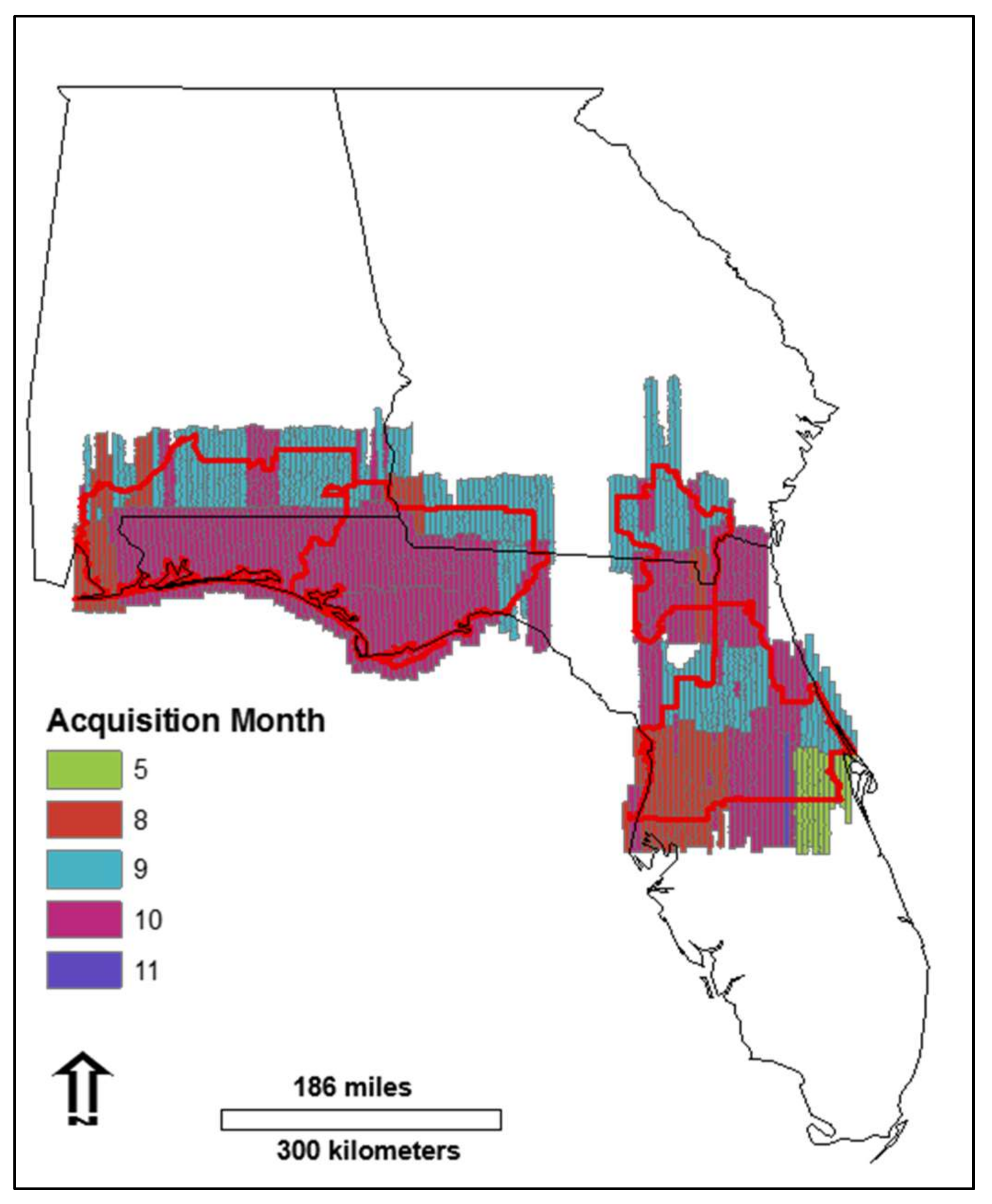
| Alabama | Leica Geosystems | ADS40 SH51 F/W VER 3.23 | August–October | 784 |
| ADS40 SH91 F/W VER 3.23 | ||||
| Georgia | Leica Geosystems | ADS40 SH51 F/W VER 3.23 | August–October | 1831 |
| ADS40 SH91 F/W VER 3.23 | ||||
| Florida | Leica Geosystems | ADS40 SH51 F/W VER 3.23 | May–November | 2371 |
| ADS40 SH81 F/W VER 3.23 | ||||
| ADS40 SH91 F/W VER 3.23 |
| Model | Class | Code | Query |
|---|---|---|---|
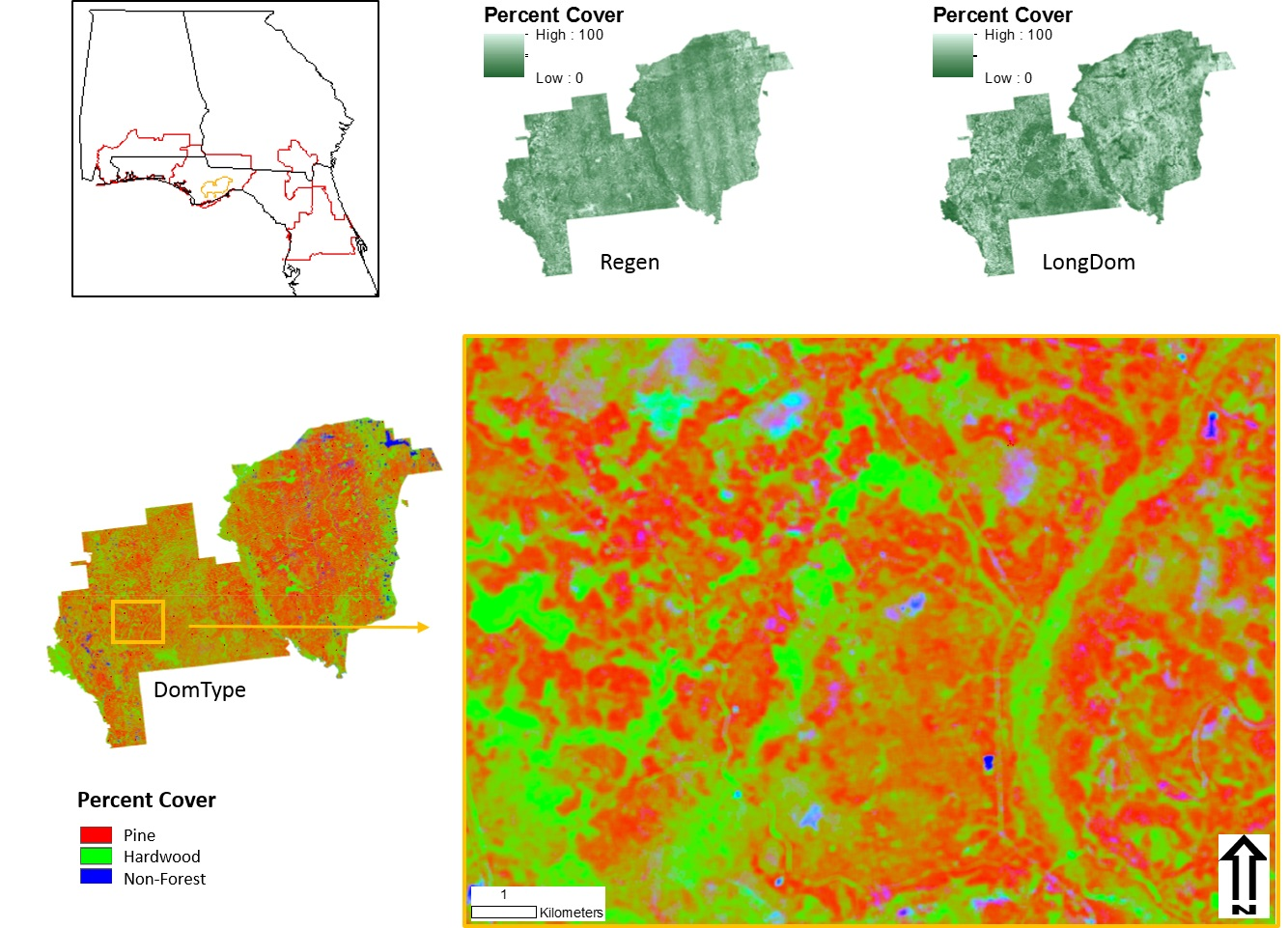
| DomType | Hardwood | 1 | (Hardwood BAA > Pine BAA) and NOT (Total TPA < 8 and TPA less than 5 in DBH < 225) |
| Pine | 2 | (Pine BAA ≥ Hardwood BAA) and not (Total TPA < 8 and TPA less than 5 in DBH < 225) | |
| NONFOR | 3 | Total TPA < 8 and TPA less than 5 in DBH < 225 | |
| Regen | Regen | 1 | (DomType < 3 and Total TPA < 20 and TPA less than 5 in DBH > 300) |
| LongDom | Longleaf | 1 | DomType = 2 AND (((Longleaf BAA)/Pine BAA) ≥ 0.5) |
| State | Model | Predictors | Train RMSE | OOB RMSE | Std. Dev. |
|---|---|---|---|---|---|
| Alabama | Pine BAA | Mean; NAIP1|Standard Deviation; NAIP4|GLCM; NAIP4|DomType; NonForest, Pine, Hardwood|Regen | 9.66 | 28.03 | 35.14 |
| Pine TPA | Mean; NAIP1, NAIP3|Standard Deviation; NAIP4|GLCM; NAIP2, NAIP4|DomType; Pine|Regen | 25.34 | 72.35 | 89.87 | |
| All BAA | Mean; NAIP1, NAIP3|GLCM; NAIP2, NAIP3|DomType; NonForest, Pine | 12.46 | 36.51 | 52.69 | |
| All TPA | Mean; NAIP1, NAIP3|Standard Deviation; NAIP4|GLCM; NAIP2, NAIP4|DomType; Pine|Regen | 25.21 | 71.79 | 99.05 | |
| Georgia | Pine BAA | Mean; NAIP1, NAIP4|Standard Deviation; NAIP4|GLCM; NAIP4|DomType; Hardwood|Regen | 7.95 | 23.17 | 30.29 |
| Pine TPA | Standard Deviation; NAIP4|GLCM; NAIP4|DomType; Pine|Regen | 18.86 | 54.8 | 67.23 | |
| All BAA | Mean; NAIP2, NAIP3, NAIP4|GLCM; NAIP3|DomType; NonForested | 13.62 | 40.2 | 52.86 | |
| All TPA | Standard Deviation; NAIP4|GLCM; NAIP2, NAIP3|DomType; Hardwood|Regen | 24.98 | 72.36 | 93.59 | |
| Florida | Pine BAA | Mean; NAIP1, NAIP2|Standard Deviation; NAIP1-NAIP4|GLCM Contrast; NAIP4|DomType; Pine, Hardwood | 8.00 | 23.38 | 31.37 |
| Pine TPA | Mean; NAIP1, NAIP2|Standard Deviation; NAIP1-NAIP3|GLCM Contrast; NAIP1-NAIP4|DomType: Pine, Hardwood | 20.53 | 59.55 | 82.27 | |
| All BAA | Mean; NAIP1, NAIP4|Standard Deviation; NAIP2, NAIP3|GLCM Contrast; NAIP1, NAIP2, NAIP4|DomType: Hardwood|Regen | 15.82 | 46.12 | 58.91 | |
| All TPA | Mean; NAIP1, NAIP4|Standard Deviation; NAIP2-NAIP4|GLCM Contrast; NAIP1, NAIP2|DomType: Pine | 27.17 | 77.87 | 103.60 |
| Model | State | Predictor variables | Average Error (Bagged) | Most Likely Class Map Accuracy (Bagged) |
|---|---|---|---|---|
| DomType | Alabama | All Mean|All Standard Deviation|All GLCM Horizontal Contrast | 23% (35%) | 76% (73%) |
| Georgia | All Mean|All Standard Deviation|All GLCM Horizontal Contrast | 20% (34%) | 76% (70%) | |
| Florida | All Mean|All Standard Deviation|All GLCM Horizontal Contrast | 23% (35%) | 74% (73%) | |
| Regen | Alabama | All Mean|All Standard Deviation|All GLCM Horizontal Contrast | 10% (11%) | 94% (94%) |
| Georgia | All Mean|All Standard Deviation|All GLCM Horizontal Contrast | 16% (17%) | 89% (89%) | |
| Florida | All Mean|All Standard Deviation|All GLCM Horizontal Contrast | 11% (11%) | 94% (94%) | |
| LongDom | Alabama | Mean; NAIP2, NAIP3|GLCM Contrast; NAIP2, NAIP3, NAIP4 | 13% (13%) | 92% (92%) |
| Georgia | Mean; NAIP2, NAIP3, NAIP4|Standard Deviation; NAIP3, NAIP4|GLCM Contrast; NAIP1, NAIP4|DomType; Hardwood, Pine|RegenProb | 6% (7%) | 96% (95%) | |
| Florida | Mean; NAIP1, NAIP3|Standard Deviation; NAIP4|GLCM Contrast; NAIP2|DomType; Pine|RegenProb | 12% (12%) | 92% (92%) |
| Model | Processing Time (h) | Storage Space (gigabytes) |
|---|---|---|
| ALL BAA | 94 | 143 |
| ALL TPA | 94 | 163 |
| PINE BAA | 94 | 99 |
| PINE TPA | 94 | 145 |
| DomType | 104 | 250 |
| Regen | 104 | 38 |
| LongDom | 78 | 32 |
© 2018 by the authors. Licensee MDPI, Basel, Switzerland. This article is an open access article distributed under the terms and conditions of the Creative Commons Attribution (CC BY) license (http://creativecommons.org/licenses/by/4.0/).
Share and Cite
Hogland, J.; Anderson, N.; St. Peter, J.; Drake, J.; Medley, P. Mapping Forest Characteristics at Fine Resolution across Large Landscapes of the Southeastern United States Using NAIP Imagery and FIA Field Plot Data. ISPRS Int. J. Geo-Inf. 2018, 7, 140. https://0-doi-org.brum.beds.ac.uk/10.3390/ijgi7040140
Hogland J, Anderson N, St. Peter J, Drake J, Medley P. Mapping Forest Characteristics at Fine Resolution across Large Landscapes of the Southeastern United States Using NAIP Imagery and FIA Field Plot Data. ISPRS International Journal of Geo-Information. 2018; 7(4):140. https://0-doi-org.brum.beds.ac.uk/10.3390/ijgi7040140
Chicago/Turabian StyleHogland, John, Nathaniel Anderson, Joseph St. Peter, Jason Drake, and Paul Medley. 2018. "Mapping Forest Characteristics at Fine Resolution across Large Landscapes of the Southeastern United States Using NAIP Imagery and FIA Field Plot Data" ISPRS International Journal of Geo-Information 7, no. 4: 140. https://0-doi-org.brum.beds.ac.uk/10.3390/ijgi7040140