Use of DEMs Derived from TLS and HRSI Data for Landslide Feature Recognition

Abstract

This paper addresses the problems arising from the use of data acquired with two different remote sensing techniques—high-resolution satellite imagery (HRSI) and terrestrial laser scanning (TLS)—for the extraction of digital elevation models (DEMs) used in the geomorphological analysis and recognition of landslides, taking into account the uncertainties associated with DEM production. In order to obtain a georeferenced and edited point cloud, the two data sets require quite different processes, which are more complex for satellite images than for TLS data. The differences between the two processes are highlighted. The point clouds are interpolated on a DEM with a 1 m grid size using kriging. Starting from these DEMs, a number of contour, slope, and aspect maps are extracted, together with their associated uncertainty maps. Comparative analysis of selected landslide features drawn from the two data sources allows recognition and classification of hierarchical and multiscale landslide components. Taking into account the uncertainty related to the map enables areas to be located for which one data source was able to give more reliable results than another. Our case study is located in Southern Italy, in an area known for active landslides.

1. Introduction

Along the marl–clay hillslopes of the Southern Apennine, the most widespread slope movements are complex slide-earthflow landslides. These landslides present an alternate kinematic behavior characterized by prolonged slow motion and shorter partial or total reactivation phases. Due to this space-time behavior, they represent a major natural threat, causing significant and continuous damage to settlements and infrastructures [1,2]. Therefore, the identification, reconnaissance, mapping and geomorphic state is fundamental for present-day hillslope stability at site and landslide hazard assessment at basin scale, requiring a multidisciplinary approach to combine the competences in geomatics, geomorphology, and geological engineering [1,3,4].

Traditional methods for producing landslide maps mainly consist of the interpretation of aerial stereoscopic photographs made by experts, assisted by field observations [5]. Such conventional geomorphological mapping is generally unable to provide a thorough and non-subjective representation of landscape complexities at different scales [6]. Current advances in automated and objective terrain analysis are based on geostatistical and geomorphometric concepts and procedures using digital elevation models (DEMs) from different data sources, processed [7,8,9] by commercial geographical information system (GIS) software packages using grid-based and/or object-oriented procedures [10,11]. Spatial variations in slope, aspect, roughness, and curvature help photo-interpreters to detect and to map landslides, especially when the movements are ancient and the landslide surfaces not straightforwardly discernible by their chromatic signature in the images [12]. Very high resolution DEMs (1-meter resolution or finer) and derivative products (for example, contour maps, shaded relief images, measures of surface roughness, and maps of slope and curvature) are used primarily for visual analysis of topographic surfaces and recognition of morphometric landslide parameters [5,13].

Over the last decade, the use of satellite data and technology for landslide investigations has been significantly increasing, mostly as a result of the increased availability of high-resolution satellite (HRS) sensors. HRS images can be draped over DEMs to obtain 3D views of terrain, which can be visually interpreted in order to detect and map landslides [14,15,16].

Review of the vast literature reveals that images taken by optical sensors are preferred for landscape detection and mapping using visual or analytical methods [17,18,19,20]. Highly detailed DEMs can be easily produced across wide areas with HRSI stereopairs and aerial laser scanners (ALS), although these are sometime not suitable for steep and rugged slopes or on smaller areas, typically including landslides, where a land-based acquisition geometry, whenever possible, allows for better description [21,22,23,24,25]. Terrestrial laser scanner (TLS) survey provides good results due to both its high point density and greater intrinsic accuracy, even if its frontal acquisition geometry limits its range of application. A few studies have used statistical measures such as semi-variograms and spatial autocorrelation for geomorphometry; both of these can provide some information about topographic variability and surface roughness [26,27,28].

However, it is important to verify that the produced DEMs have a high accuracy in addition to their high resolution. Kriging, like other interpolation methods, allows us to produce a map showing errors associated with the built DEM. In the literature, DEM accuracy is often estimated by comparing a sample of elevation values extracted from DEM with the corresponding values actually measured on the ground through topographic technique or using cross validation [29,30,31]. The accuracy of the parameters derived from DEM is frequently evaluated using Monte Carlo methods [32,33], but this requires the use of an a priori model for DEM error analysis.

For validation and calibration of landslide hazard and risk assessment, an integrated procedure in objective geomorphological mapping, based on a hierarchical, multiscale step-by-step and training-target approach, has been proposed in the literature [6] and also discussed within the international geomorphological community [34]. For landslide field study at a regional scale, Coico [35] has proposed an extended approach of landslide analysis and mapping, focusing on the use of hierarchical generalization that can be used as a first operative step [36].

In our paper, we discuss how to compute and make use of the uncertainty of DEMs and derived products, starting from data provided by HRSI stereopairs and TLS surveys. We suggest a methodology for assigning uncertainty to the elevation value of each node of a DEM and then propagating it to derived products (for example, slope) in order to delimit the extension of the reliable area for analysis. We used the kriging algorithm to interpolate data, which also produces an estimate of DEM interpolation error as its output. The accuracy of DEM-derived products was estimated through propagation of error starting from the DEM uncertainty after the covariance matrix was modelled.

Applying the same procedure and the same codes to two different datasets allows us to highlight differences in the results due to intrinsic characteristics. Our assessment of the uncertainty of the elevation and of the DEM-derived parameters allows us to bound the extension of the areas within which we expect to be able to perform a reliable analysis.

The purpose of this paper is to show how a detailed and accurate knowledge of local topography can improve landform characterization mapping. Using the method described above, this research aims at understanding the spatial characteristics of a highly hazardous landslide complex, analyzing the relationships between geomorphological parameters and landslide events. The landslide we studied is located in a well-known landslide district, the Pisciotta–Ascea coastal landscape in the Tyrrhenian borderland ecoregion in southern Italy [37].

2. Test Case and Data

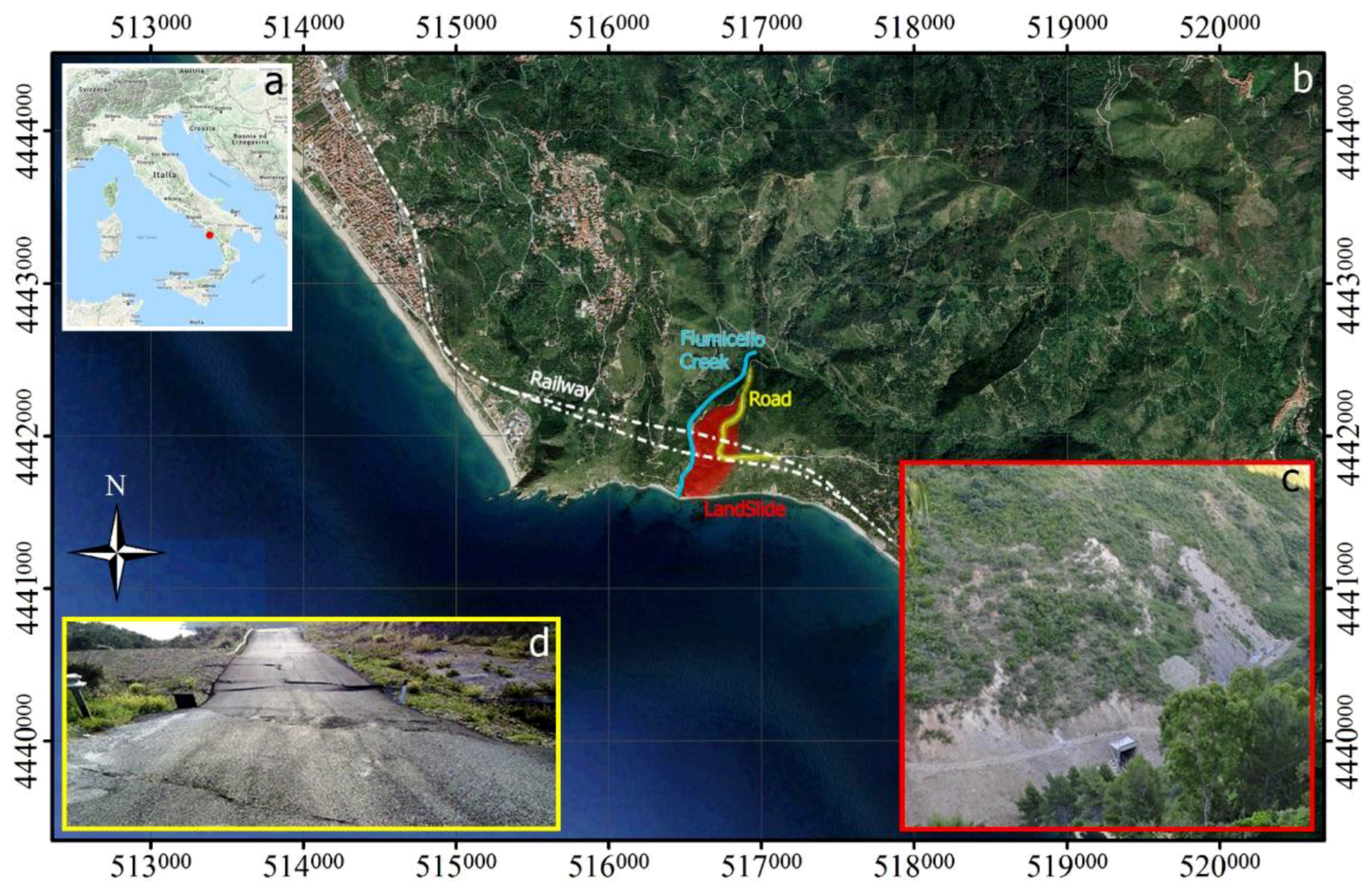
2.1. Test Case

The landslide case study is located in Pisciotta municipality (southern Italy) on the left side of the valley along the final portion of the Fiumicello Creek. Landslides cause extensive damage both to the important Palinuro state road and to the two sections of the railway line connecting north and south Italy [38]. The consequences of these movements are visible on a long stretch of road that appears to be progressively disrupted. In December 2008, due to a sudden reactivation landslide event, the railway was endangered and disrupted by a landslide-caused dam break. This landslide system (Figure 1a–d) is a well-known reactivated, deep-seated, slow-moving slope mass movement in the Cilento, Vallo di Diano and Alburni (CVDA) UNESCO global geopark; hence, it was selected as one of the most relevant prototypal moving geosites by the Geopark Scientific Committee [35]. Topographic and geotechnical monitoring campaigns carried out from 2005 to 2009 showed that the landslide moved about 0.5 cm/day horizontally, and vertically about 0.2 cm/day [39,40].

Two different datasets were used to study the behavior of this landslide: satellite stereo images, which require complex procedures to process the data; and terrestrial laser scans, which require careful planning and accurate editing. TLS data were acquired in June 2011 using the long-range TLS Riegl VZ400. Six months later, we acquired a GeoEye-1 stereo image pair covering an area of 110 km², inclusive of the landslide. The image was captured in reverse scan mode and recorded the panchromatic band and all four multispectral bands. For our analysis, only the panchromatic imagery was used.

The topography of the area covered by the stereopair is highly variable, ranging from sea level to altitudes of over 1000 m. Shrubs and isolated large trees cover most of the area; however, there are also a few residential zones and isolated houses.

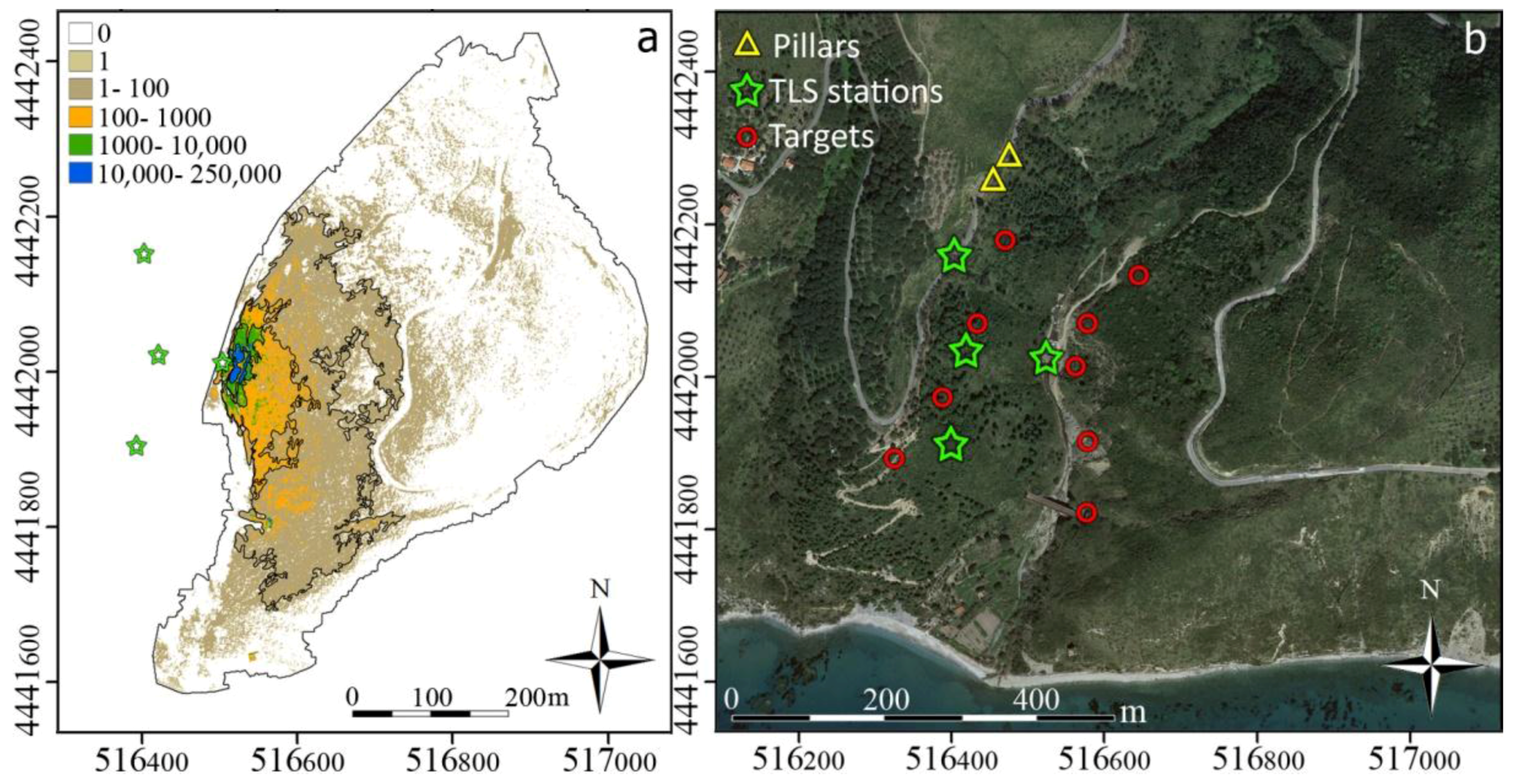
2.2. TLS Data

Data acquired through TLS required several processing steps. Many of them are of a critical nature in terms of obtaining good results. Multiple overlapping scans were needed to survey the entire landslide area. The rugged morphology of the surveyed area was a major factor in our choice of sites for placing stations and artificial targets. We recorded laser scan measurements acquired from several TLS stations located on stable locations (as highlighted in the hazard maps of the local river basin authority) at different altitudes along the opposite side of the valley in order to measure both the upper and the lower parts of the landslide downstream. Some of the characteristics of terrestrial laser scanner (Riegl VZ-400) used to acquire data, are listed in

Table 1. A few characteristics of the TLS used.

Riegl VZ400
Min. range (m)	1.5
Max. range (m)	600
Beam diameter at exit (mm)	7
Beam divergence (mrad)	0.3
Spot at 50 m distance (mm)	18
Max. Horiz. Field of view (deg)	360
Max. Vert. Field of view (deg)	100
Min. Horiz. & Vert. step size (deg)	0.0024
Max. measurement rate (KHz)	300
Uncertainty of Horiz. & Vert. Step size (deg)	0.0034
Software name	RiscanPro

.

We used nine spherical targets for co-registration between scans and for georeferencing the global-aligned point cloud in a given reference system. The combined total of points is about 110 million. The distance between TLS stations and the reflecting surface of the ground ranged from roughly 50 to 600 m. Since the angular sampling step of the laser beam was kept constant, the distances between the points on the ground in the laser beam’s direction, being a linear function of the distance between the laser station and the ground, were highly variable. Very high return point density was observed in the close vicinity of the scanning stations and in overlapping areas. However, the return point density at the boundaries of the survey area was low to the point that it could no longer be used to develop a reliable terrain model using interpolation techniques [41,42]. The slope causes point density to be higher at the toe of the landslide, nearest to the TLS stations, and lower in the upper part. The density distribution map is shown in Figure 2a.

The coordinates of both the targets and the TLS stations were measured by global navigation satellite systems (GNSS) receivers in static mode, keeping fixed the coordinates of two vertices marked by steel pillars firmly placed on a concrete wall in a stable area. The distance between targets and pillars ranged from a few dozen to a few hundred meters. The two pillars were connected to two permanent stations (PS) 26 km (Castellabate) and 38 km (Sapri) away from the landslide in the network of the Campania Region for Network Real Time Kinematic (NRTK) service. Due to the great distance between the landslide area and the PS, we made continuous daily GNSS observations. This allowed us to frame the LiDAR survey into a stable and continuously monitored reference frame. The reference system adopted was the national one, the European Terrestrial Reference Frame 2000 (ETRF00).

The positions of pillars, TLS stations, and targets are marked, respectively, with yellow, green and red symbols in Figure 2b. The final coordinates of the targets were derived through least squares adjustment in ETRF00.

Single scans with an amount of overlap ranging from 40% to 80% were co-registered and georeferenced using the Polyworks software package by Innovmetric (2014) [43]. Co-registration of overlapping scans is a very crucial step to avoid distortion between adjacent clouds and to preserve geometric relations between the points of the two clouds. Co-registration was performed with a Polyworks tool based on the iterative closest point (ICP) algorithm, and by using a six-parameter rigid-body (affine) transformation.

The resulting aligned global scan required editing to remove all points not belonging to the bare soil from the dataset. In our application, this mostly concerned vegetation, but also included some artifacts. To perform the manual editing of the point cloud, we used Cloud Compare open-source software (ver. 2.8.1) [44]. The georeferenced point cloud was cut into a number of tiny strips, which were shown in cross-section in order to better locate those points not belonging to bare earth to be removed from the dataset.

In order to georeference all of the scans, an affine transformation was performed and compared with a seven-parameter Helmert transformation. The values of the rotations (in decimal degrees) were measured up to the fifth decimal digit. The values of the translations differed by 1–5 mm, and the scale factor was 0.99986. The georeferencing residuals were less than 10 cm. Their mean was 4 cm. The finished process produced a point cloud describing the edited and georeferenced landslide surface.

2.3. TLS Stereopair Satellite Images

The test case GeoEye-1 images have a nadiral ground sampling distance (GSD) of 0.5 m and a radiometric resolution of 11 bit. They were acquired on 1 January 2012 at 09:43 Greenwich Mean Time (GMT). A few characteristics of the stereopair are listed in

Table 2. Characteristics of the GeoEye-1 stereopair.

Product Line		Geostereo
Product pixel size		0.5 m
Nominal GSD cross scan		0.462 m
Nominal GSD Pan along scan		0.485 m
Scan azimuth		0.605°
Scan direction		Reverse
Left Stereo		Right Stereo
Collection azimuth	65.3446°	Collection azimuth	151.9583°
Collection elevation	69.35349°	Collection elevation	64.86915°
Sun angle azimut	160.0611°	Sun angle azimut	160.2717°
Sun angle elevation	24.20402°	Sun angle elevation	24.25851°
Acquisition date	2012–01–01	Acquisition date	2012–01–01
Acquisition time	09:43 GMT	Acquisition time	09:44 GMT
Cloud cover	0%	Cloud cover	0%

.

Every image has unique sensor model parameters that reflect its location, orientation, and other information at the time the image was collected. Metadata associated with the image provide the parameters required to specify from which sensor a given image has been captured.

For the georeferencing of images and to obtain our stereo model, we used the software package Socet GXP ver. 4.2.0 by Bae Systems [45], which implements a rigorous sensor model. The ground control points (GCPs) were surveyed with GNSS receivers in NRTK mode. To obtain a homogeneous distribution of well-matched points, we designed a network whose vertices are in close proximity to the nodes of a regular grid.

Thanks to the high speed of the NRTK survey, we were able to measure more points near the nodes, allowing us to choose points having the best correspondence on the image and the best measurement accuracy. We field-measured 33 GCPs, of which 24 were used for georeferencing the image. The referencing system we used was the ETRF00 with ellipsoidal heights.

In order to build the DEM, from the matching algorithms implemented in Socet GXP, we used the automatic spatial modeler (ASM) algorithm, which is recommended for the extraction of dense 3D point clouds from stereo images in highly vegetated areas at different elevations. This algorithm is the only one available in commercial software that can output a 3D point cloud in place of a grid DEM, making it possible to choose the interpolation algorithm to build the DEM at a later time.

The digital surface model (DSM) from the stereo pair of images was a georeferenced 3D point cloud of the area inclusive of both vegetation and buildings. To derive a bare earth digital terrain model (DTM) from the DSM, we used the cloth simulation filter (CSF) plugin, developed for filtering LiDAR point clouds, with the open-source software Cloud Compare [46]. This tool requires the definition of some input parameters; for our purposes, the most effective were choice of scenery (for example, steep slope, relief, or flat terrain), grid size, number of iterations and classification threshold. To define the proper values for these parameters, we performed several tests, before finally choosing ‘steep slope’ as scenery, with a classification threshold of 0.9, a 1 m grid size, and 1000 iterations. The quality of the process was monitored trough 3D stereoscopic vision.

A software-generated numerical value called figure of merit (FOM), ranging from 0 to 99, was used to estimate matching accuracies. In dark or shadowy areas of the image, the FOM ranges from 20 to 40; it is good practice to keep only those points with a FOM value above 40. In highly vegetated areas where the filtering algorithm did not succeed, or in shadowed areas where the digital matching did not work (having a low FOM value), we integrated the point cloud with other manually plotted points, using a digital stereo photogrammetric workstation.

Figure 3a shows one of the stereopair images with the distribution of GCPs (small red circles), whose east (E), north (N), and height (h) georeferencing residuals are shown in Figure 3c. Figure 3b,d shows the FOM values (Figure 3b) computed for the entire image and a zoomed view of a small area including the landslide (Figure 3d). The matching algorithm does not work well in shadowed areas. There, the FOM values are quite low. In the narrow area, the part of the image where the FOM values are poor was edited as described above. In highly vegetated areas, the filtering algorithm fails to divide the points into the two categories of bare ground and non-ground. In contrast, in areas with medium dense vegetation, the algorithm was able to optimally subdivide ground points from those offground.

Figure 4a–c shows the part of the area subjected to filtering: Figure 4a shows the matched points that form the DSM, Figure 4b shows the ground points after applying the filter, and Figure 4c shows the points manually measured in stereo mode using a digital workstation, shown as 1609 white dots. The final point cloud was made of the bare earth points plus the manually plotted ones. Using this set of points, we built a DEM as described in Section 3.1 and Section 4.1, below.

For testing purposes, we built a non-uniform rational basis spline (NURBS) surface using the tool Rhinoresurf plugged into the CAD software Rhinoceros version 5 [47]. Figure 5 shows the NURBS surface built based on the following parameters: 3rd degree, 300 points in both directions (which formed a square mesh of nearly 5 m), and a tolerance of 1 cm.

3. Methods

Our proposed method requires both a TLS-derived point cloud and a 3D model derived from the HRSI stereopair and expressed as a point cloud in order to apply the same interpolation algorithm to both datasets for direct comparison.

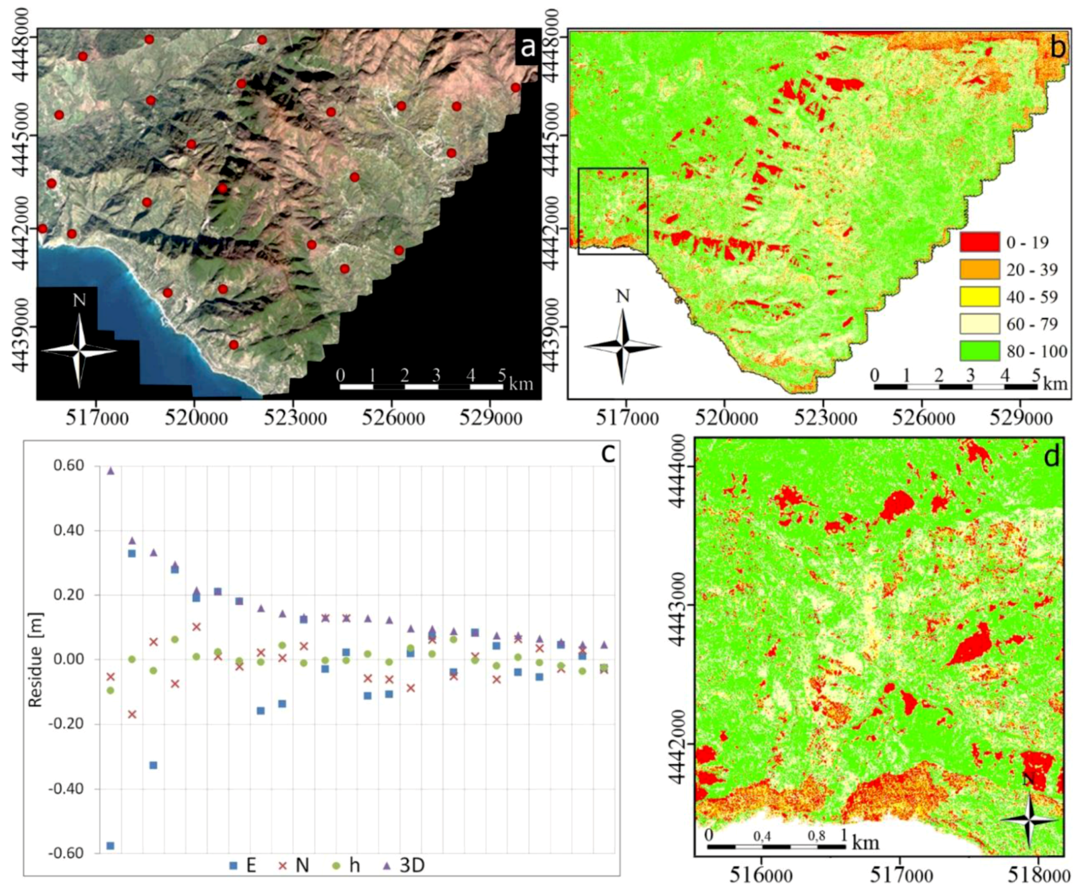
3.1. DEM Construction and Related Error Analysis

To generate the grid DEM once the point clouds have been georeferenced, one must choose a proper interpolation method and define relevant parameters, such as the grid size and the search radius around each node. These parameters depend highly on the specific characteristics of the spatial distribution and density of each point cloud.

The cloud obtained from the HRSI stereo pair (see Section 2.3) generally presents a regular point (corresponding to pixel) density over the entire area encompassed by the stereoscopic model—at least before vegetation filtering. In the case of TLS point clouds, the high variability in point density makes the choice of the parameters less straightforward. In a TLS survey, point density quickly decreases with distance from the stations, as shown in Figure 2a for our test site.

The choice of algorithm parameters can be aided by cross-validation and assessment of the quality of interpolation performed by each set of values to be compared [41]. Using our data sets, we randomly extracted a sample of validation data (5%, used for testing) and fitted the remaining part (95%, used for training) on a grid DEM. Then, we computed the differences between the elevation values of each sample point and its corresponding forecast value from to the DEM. We computed a few parameters of the distribution of our testing sample—mean and mode, as well as variance and mean absolute deviation—to evaluate the accuracy of the fitting method [41]. The cross-validation process was run on both data sets.

Given that the spatial distribution and density of the points influence the accuracy of the DEM, it is worthwhile performing a trend analysis of the elevation. Given a set I of N pairs P_i (x_i, y_i, z_i), P_h (x_j, y_j, z_j), with difference of position ∆ = (∆x, ∆y), the empirical variogram is [48]:

$$g(\Delta x,\Delta y)=\frac{1}{2N_{\Delta }}{\displaystyle \sum _{(i,j)\in I_{\Delta }}(z_i}-z_j{)}^2$$

(1)

For the case study, the direction of the maximum gradient corresponds roughly to the x-axis of the reference system (0° east), while the y-axis (+90° north) is oriented along the river bed.

We ran cross-validation tests on the sets of interpolated values obtained through both the kriging and the inverse distance-weighted (IDW) methods, where the weight was chosen to equal the inverse of the squared distance. Since the results were similar, we chose to proceed with kriging, because it has the advantage of providing output on not only the grid of the heights estimated from the points, but also the grid of the standard deviations of these estimates. This latter allows one to draw a map of the heights’ uncertainty [41]. A number of widespread software packages, for example Golden Software’s Surfer, can perform this function [49].

The map of the estimated standard deviations of the heights can be used for identifying areas of greater uncertainty and defining the boundaries areas within a sufficient degree of reliability once a threshold has been chosen. For our test case, that threshold was 5 m. At the borders, standard deviation would typically reach very high values, due to the presence of fewer points. These two aspects are very important in TLS surveys, because point density decreases dramatically at the borders of the surveyed area, and because this decrease is irregular, thus not permitting an objective definition of its boundaries. Conversely, for HRSI, the data distribution, not being limited by the range of an instrument, is uniform over the entire model. The DEM can have a few holes in mountainous areas, where the matching algorithm does not work because of shadow effects (regions inside the model where heights are set to a no data value), or in highly vegetated ones. These data gaps must be edited.

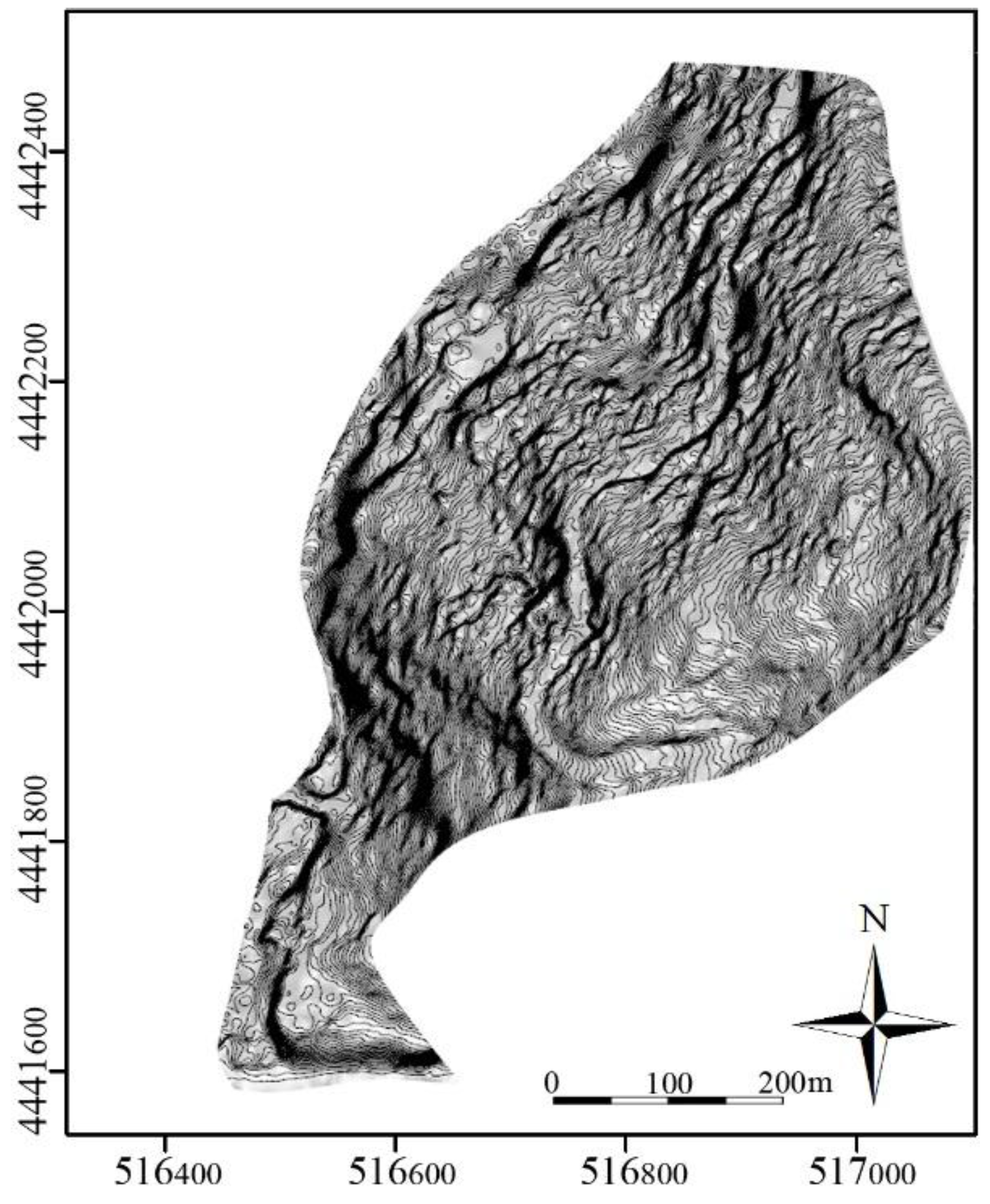
3.2. DEM-Derived Maps (Slope and Aspect)

It is possible to automatically extract from the grid DEM not only a contour map, but also other parameters of geomorphological interest, such as slope and aspect. Several formulas have been proposed [50] for computing slope and aspect; in applying the variance–covariance propagation law, we used formulas that took into account only the four neighboring points in the west–east and north–south directions, indicating these points with the letters W, E, N, and S.

Given these considerations, slope (P) and aspect (T) can be computed in radians as:

$$P=\arctan \sqrt{{\left(\frac{z_E-z_W}{2\Delta x}\right)}^2+{\left(\frac{z_n-z_s}{2\Delta y}\right)}^2}$$

(2)

$$T=\mathrm{atan}2\left(-\frac{z_n-z_s}{2\Delta y},-\frac{z_E-z_W}{2\Delta x}\right)$$

(3)

where subscripts W, E, N, and S respectively indicate neighboring points in the west, east, north and south.

To compute the uncertainty associated with the features derived from DEM, several authors have suggested the use of the Monte Carlo method [33,51], but this implies the a priori definition of the error model associated with the interpolated heights. Therefore, we chose to directly use the error map derived using the kriging algorithm. Uncertainty estimates for some parameters, such as slope and aspect, can be computed using the standard deviation of the kriged data by using the formula for error propagation.

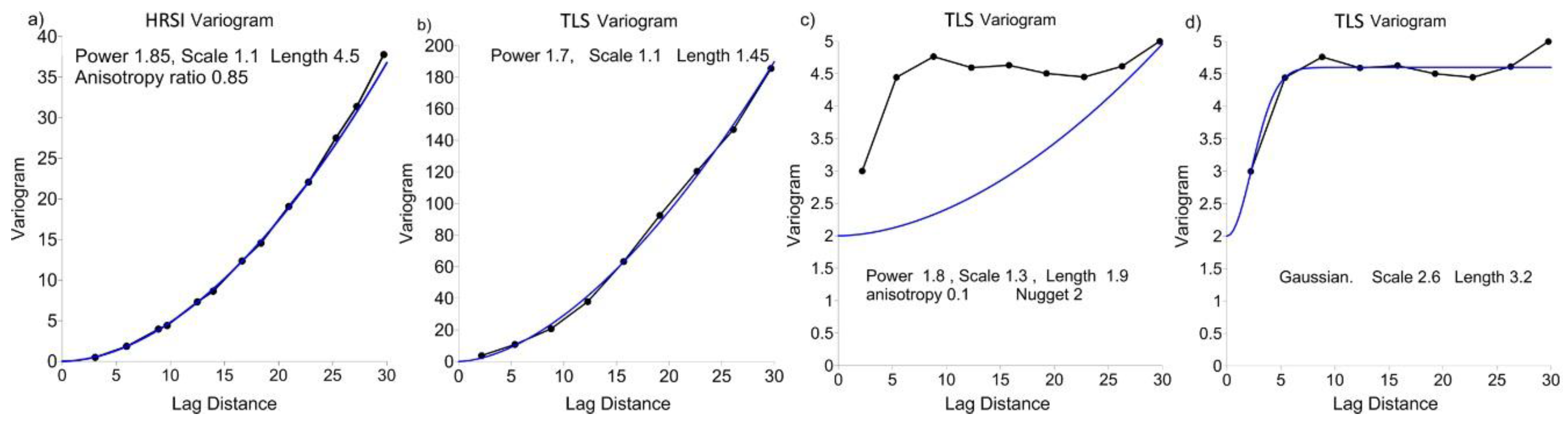
Propagation of Error in Slope and Aspect Maps

Equations (2) and (3), which express a relationship between the considered parameters and the heights of the neighboring points, have the form:

$$f=f(z_W,z_E,z_S,z_N)$$

(4)

The variance of geomorphometric parameters can be derived from the variance–covariance propagation law [52]. Indicating the variances associated with the nodes with ${\sigma }_W^2, {\sigma }_E^2, {\sigma }_S^2, {\sigma }_N^2$, the covariance between nodes i and j with σ_ij, and the height differences with ${\delta }_E=z_E-z_W$, ${\delta }_N=z_N-z_S$, assuming square pixels, and introducing the linear correlation coefficients ρ_ij so that ${\sigma }_{ij}={\rho }_{ij}{\sigma }_i{\sigma }_j$, it is possible to express the variance of the slope S as:

$$\begin{array}{cc}\hfill \mathrm{var}(S)=& {\left(\frac{1}{1+S^2}\right)}^2\frac{{\delta }_E^2({\sigma }_E^2+{\sigma }_W^2)+{\delta }_n^2({\sigma }_n^2+{\sigma }_s^2)}{{\delta }_E^2+{\delta }_n^2}+\hfill \\ & +\frac{2\rho }{{\delta }_E^2+{\delta }_n^2}\left[-\text{}{\delta }_E^2{\sigma }_E{\sigma }_W+{\delta }_E{\delta }_N({\sigma }_E-{\sigma }_W)({\sigma }_N-{\sigma }_S)-{\delta }_N^2{\sigma }_W{\sigma }_S\right]\hfill \end{array}$$

(5)

Aspect, given in Equation (3), has a variance given by:

$$\begin{array}{l}\mathrm{var}(T)=\frac{1}{\text{}{(\delta z_E^2+\delta z_N^2)}^2}\left[\delta z_N^2{\sigma }_E^2+\delta z_N^2{\sigma }_W^2+\delta z_E^2{\sigma }_s^2+\delta z_E^2{\sigma }_N^2\right]+\\ +2\rho \frac{1}{\text{}{(\delta z_E^2+\delta z_N^2)}^2}\left[-\text{}\delta z_N^2{\sigma }_E{\sigma }_W+\delta z_E\delta z_N({\sigma }_W-{\sigma }_E)({\sigma }_N-{\sigma }_S)-\delta z_E^2{\sigma }_W{\sigma }_S\right]\end{array}$$

(6)

Note that Equations (5) and (6) are rigorous, because the linear correlation coefficients represent the contribution of the covariances. This is critical in defining the resulting variance. While the variance of each node comes from the standard deviation of the heights interpolated using kriging, computing the covariance is not trivial and is not performed by commercial software packages. Yet given that the contribution of the covariances is not negligible, it must be taken into account.

We propose to express the covariances in Equations (5) and (6) by means of the standard deviations and linear correlation coefficients between the heights of the nodes and to determine this value through the empirical variogram, i.e.,:

• to deduce from the variogram a linear correlation coefficient ρ(d) for a lag d corresponding to the distance between the nodes, which is a function of the grid size D;
• to consider the same linear correlation value for all pairs of nodes at the same distance d.

Given these hypotheses, it is possible to compute also the covariances between adjacent nodes. To automate computation, we developed a script that:

• reads the input grids in textual format, taking into account the ‘no value’ nodes eventually present in the standard deviation grid provided by kriging;
• applies the above equations for all nodes except for those with undefined neighboring nodes;
• computes the new grids of the DEM-derived parameters and relative uncertainties.

Those areas where the standard deviation of the heights is not computed by the kriging algorithm (‘no value’ areas) obviously lead to even more extended areas for which it is also not possible to compute the standard deviation of the derived parameters.

3.3. Criteria of Geomorphological Mapping

Contour maps with equidistance between the contour lines of 1 m, along with maps of the main geomorphological characteristics, are often used as base maps for geomorphological mapping. Based on landscape features, a number of meaningful classes of geomorphological parameters can be appropriately defined.

In order to validate our products, an expert qualitative geomorphological validation of both the base maps and the geomorphometric-derived maps was used. The expert-based judgement was based on multi-temporal field-based surveys and was supported by preliminary object-based geomorphological mapping on training landforms, in accordance with the procedure suggested by Dramis et al. (2011) [6]. For this paper, a new GIS-based, full-coverage, object-oriented geomorphological mapping system developed by the Salerno University was used. This GmIS_UniSa Mapping system has been used by several Italian engineering, landscape ecology and hydro–geomorphological projects.

Following this procedure, we compared the base topographic maps built with TLS and satellite data with the actual morphological detection of training surficial features. We focused on selected landslide components: head scarps, lateral scarps, hummocky landslide bodies, and en-echelon longitudinal scarps. These components have been used by Fleming et al. [53] and Parise [54] for analytical landslide mapping, in which the detection of a few significant surficial features on active/reactivated landslides allows recognition of the complex kinematics of the landslide components, including element displacements and movements.

The expert-driven judgement gave us insight into slope class definition as a basic geomorphometric parameter, based on the slope class distribution in each of the above-mentioned landslide components. These criteria follow previous qualitative and quantitative geomorphological approaches and procedures regarding landslide reactivations at the regional scale, carried out on a number of selected sites of the Southern Apennines [55]. At these sites, along with the mid-term morpho-evolutive sequence reconstructions, quantitative observations of distinctive kinematic geomorphic indicators and surface features, along with landslide analysis, could provide knowledge of the kinematics of landslide evolution. Therefore, comparative analyses were performed using the following steps:

(1)

Step 1 concerns traditional field-surveyed, symbol-based geomorphological mapping of the study landslides and the surrounding landslide-prone areas.

(2)

Step 2 ‘translates’ Step 1 into a bounded, full-coverage geomorphological map, delimiting and coding the geomorphological features into geomorphological units defined by nodes, boundary lines, polygons, and related topological rules [6]. Topographic optimization of the data fusion of the TLS point cloud with GeoEye images is used to characterize the above hierarchical landslide units by significant multiscale geo-morphometric analysis.

This procedure could constitute the training phase for automatic object-based landslide unit segmentation and classification.

4. Results

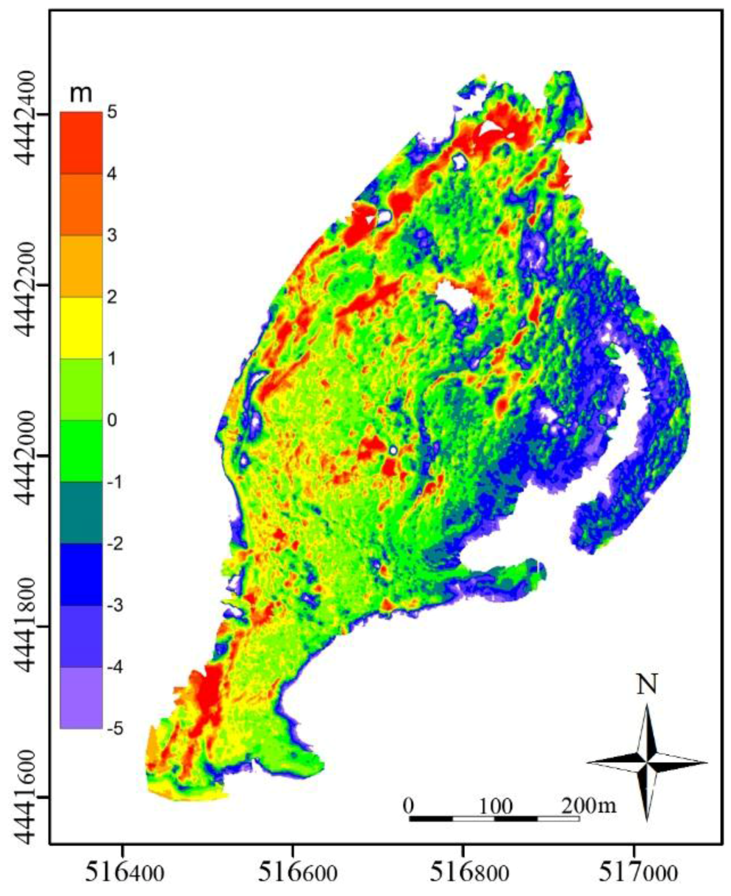
4.1. Production of DEM

The characterization of point density and distribution in the two point-cloud datasets obtained from TLS and HRSI can be performed through analysis of their variograms. This allows us to choose a proper model for assigning weights to data values neighboring the interpolant. In both cases, the obtained empirical variograms can be modeled using a power function for short lags (up to 30 m) to define the proper search radius around the node.

It is important to note that the data in these two datasets present quite different spatial behaviors, in particular concerning the anisotropy. For the HRSI data, a power model fits the empirical variogram very well in both directions (0° and 90°), introducing an anisotropy value of 0.85 (Figure 6a) (other parameters: power = 1.85, scale 1.1, length = 4.5). For TLS data, a similar power model only fits the empirical variogram for 0°, as shown in Figure 6b (power model parameters: power = 1.7, scale 1.1, length = 1.45). The result for the power model with the same or similar parameters applied to empirical data in the 90° direction is shown in Figure 6c: no fit at all. To obtain a good fit in this direction, a Gaussian model must be applied. (Figure 6d, scale 2.6, length = 3.2).

A search radius of 20 m (that is, 20 times the grid size) is sufficient to study the semivariograms for slightly higher lags; we chose a maximum lag of 30 m, which is sufficient to display the trend. The cloud derived from the HRSI stereopair was clipped in its northeastern region; this part exceeding the extent of the TLS data.

Once both the model and parameter values for this interpolation model were chosen, the two clouds were interpolated using block kriging, without drift, with a grid size of 1 m and a search radius of 20 m. We used the block kriging interpolator instead of point kriging because, according to some authors [56], the former provides not only smoothly interpolated results, but also better variance estimates.

A grid size of 1 m was deemed to be the most suitable for allowing direct comparison and interoperability between DEMs derived from such different data sources. The TLS cloud was able to allow a finer grid size (even while reducing the interpolated area because of low point density at the borders), but we believe that such a resolution would be excessive for the description of a landsliding slope.

4.2. Geomorphological, Expert-Basd Accuracy Assessment

The 1 m contour maps were the main source for our detailed geomorphological analysis, along with the derived maps of the geomorphological features. In order to geomorphologically compare the contour maps with the DEM-derived ones, we analyzed only those landslide components that are readily evident in the obtained products.

Figure 7a–d shows the contour maps obtained from TLS (Figure 7a) and HRSI (Figure 7c) data; the relative maps of height uncertainty overlaid on the contours are shown, respectively, by Figure 7b,d. The standard deviation maps allow us to objectively define the boundaries of the areas where computed elevation values can be considered reliable. Once a threshold for the standard deviation value at the borders of the map is defined, it is possible to delete data outside of the border, using map algebraic operators in a GIS environment. Analogous operations can be performed for the slope and aspect maps as well.

Looking at the uncertainty maps of DEMs derived from TLS data, it is clear that no values of standard deviation are computed for a large area at the east. This corresponds to the most elevated part of the landslide, which is characterized by a lower data density value. We decided to define as ‘no data’ those areas where standard deviations were extremely high, that is, greater than 5 m. The choice of this threshold is discussed in Section 5.

Delineation of a number of landslide entities—landslide system, landslide complexes and landslide units—overlaps the contour maps. In the legend to Figure 7a–d, these are indicated by the numbers 1, 2, and 3 for both TLS data (Figure 7a) and HRSI data (Figure 7c). The most significant and relevant landslide components are depicted as head scarp (4), lateral scarp (5), or en-echelon fracture sets (6). In addition, a few relevant landforms are highlighted; for instance, the portion of landslide-unaffected hillslope (7), which is progressively reduced by retrogressive and enlargement of the landslide boundaries; the Fiumicello streambed (8), where down-cutting erosion affects the landslide system toe; and landfill deposits from rail tunnel excavation (9).

With regard to the standard deviations for the heights (Figure 7b,d), the expert- and field-based judgments allowed us to identify ‘no data’ and neighboring areas, induced by the shadow effect (SE), as depressions, ponds, or back-slope features, by non-instrumentally-detected areas (NDA) or, simply, as a consequence of the boundary effects (BE) of the surveyed and processed area. Other areas of high uncertainty are the road (R) and the adjacent scarps.

The same geomorphological interpretation (and expert-based accuracy assessment) was performed using the DEM-derived slope and aspect maps. Comparing statistics extracted from the slope and aspects maps obtained from these two different data sources helped in detecting landslide boundaries, delimitating landslide components, and identifying characteristic geomorphological features. As regards the slope maps, in order to decide the number and size of the classes, we analyzed slope spatial frequency distributions, as shown in Figure 8.

The adopted chromatic scale describes the ranges of the six classes of slopes that were chosen. Figure 9a–d shows the slope maps for TLS data (Figure 9a) and for HRSI data (Figure 9c).

An expert-based geomorphological interpretation of slope maps is also shown, focusing on the landslide components cited above. In addition to the geomorphological interpretation, TLS (Figure 9a) and HRSI (Figure 9c) data allowed identification of roads, streambeds, natural terraces, and artificial terraced landfill, all at slopes of 5–10°, as expected. Deeply deformed, hummocky landslide bodies and landslide complexes are dominated by 10–20° slopes, with alternating 20–35° slopes. Class clusters are dominated by 35–45° slopes, and some slopes in the previous classes characterize the stepped reactivated landslide body, as shown in Figure 9a, as well as the degraded head and lateral landslide scarps. Active landslide scarps are dominated by slopes between 45 and 60°. The highest slope classes typify road scarps and river cut banks.

Different patterns of the above slope class ranges are clearly visualized on the slope maps for TLS data and HRSI data. Along with the previously explained considerations regarding the different acquisition geometries, differences in the slope maps likely also depend on different deformation and failure styles, following an observed decrease in reactivation activity after about six months.

The maps of the slope standard deviation (Figure 9b,d) show the results of the analysis based on field evidence, following the same criteria followed for contour maps. In creating the standard deviation maps, we have chosen to give more evidence to low-value classes, while higher values of uncertainty are collapsed into a single class.

Similar expert-based geomorphological accuracy assessment was performed for the aspect maps by means of analysis and visual comparison between the significant value range and the main landslide features derived from field surveys (Figure 10a–d). Results for TLS and HRSI data, respectively, are shown in Figure 10a,c; their relative standard deviations are shown in Figure 10b,d. The geomorphological analysis of the aspect maps was orientated instead towards detecting spatial patterns (lineations, crenulations, and undulations) significant for surface expression of different kinds and rates of land movements.

The surficial aspect expression of both TLS and HRSI surveys highlights the NNW block-slide rotation of the deepest failure planes in comparison with the whole landslide system. Complex intermediate landslide movements are controlled by failures along litho-structural elements, generally dipping NW and barely influenced by topography. In contrast, the direction of movement of surficial reactivated landslides is controlled by topography.

5. Discussion

The inherent structures of the TLS and HRSI surveys provide deeply different datasets for information density, extent of the covered area, and acquisition geometry. Even if we tried to process both datasets as similarly as possible, the two DEMs and the DEM-derived products differ slightly, as shown in Figure 11. The differences between DEMs can be emphasized using the obtained height difference map by subtracting the TLS DEM grid from the HRSI one.

Considering an average kinematic of a few millimeters per day, a six-month gap between the two datasets is not sufficient to explain height differences of up to several meters. Differences between the two DEM grids are due to the uncertainties of interpolated heights that, as shown in Figure 8b,d, are particularly high at the borders and in the upper parts of slopes. In contrast, for the wide central area of the slope, height differences are just 1 or 2 m; hence, they should be considered to be fully compatible with the uncertainties associated with both of the input heights in that area.

Apart from border effects in the TLS dataset interpolation, these discrepancies depend on the density and distribution of input points, as determined by acquisition geometry. The density and distribution of the point cloud derived from satellite imagery is constant (apart from the few areas where correlation did not work well or where there are holes due to vegetation editing), whereas the TLS point clouds are characterized by very high variability in density and distribution.

To investigate these differences in DEMs and derived products, we chose kriging as the interpolator only because it allows an evaluation of the interpolated height uncertainties by considering input value variabilities, which also depend on point density and clustering. As concerns the extraction of a DEM from a point cloud, we observe that other interpolators also achieve degrees of fit of similar quality, as verified through cross-validation and by evaluation of the statistics of the residuals in the heights of the checked sample. Other algorithms, however, do not allow computation of the standard deviation of interpolated heights, the knowledge of which is of primary importance for our methodology. Kriging computation combines quality of interpolation with the ability to generate an uncertainty map for estimated heights. Note also that even if it were possible to obtain an overall estimate of the several error sources that affect input data, commercial software packages generally lack a DEM interpolator that quantifies the intrinsic precision of each node.

The high standard deviation values at the boundary of the maps are very useful for defining a landslide boundary area suitable for analysis. Since for landslide areas far away from border and shadow areas (where there are known border effects and issues in interpolation) the uncertainty associated with interpolated heights ranges from 1 to 2 m (as shown in Figure 8b,d), we deem a threshold value of 5 m (that is, 2.5 times the standard deviation, a significance level of less than 1%) to be indicative of some local anomaly not dependent only on casual errors. To define the area to analyze, it is sufficient to exclude those nodes that are beyond the chosen threshold by setting them at ‘no value’. Additionally, analysis of the height uncertainty maps allows identification of the boundaries of the area within which it is more convenient to consider information coming from the TLS DEM instead of the HRSI one, given their different acquisition geometries and the differences in processing the two datasets.

In fact, the TLS DEM is more precise than HRSI DEM on that part of the slope facing and nearest to the stations. In contrast, the HRSI point cloud, presenting a more regular density of information, produces a DEM that allows analysis of a wider region with an acceptable level of uncertainty, notwithstanding some problems in areas with poor image matching. To overcome these limits, it might be possible to algebraically combine the two DEMs, which share the same grid size and extent, along the boundary given by the reliability limit of the TLS grid. This operation, performed without resampling, requires that the grids to be combined share the same extent and spacing. For our data model, a 1 m grid size DEM (along with its height uncertainty map) was identified as the proper common basis for the integration of the information coming from the two datasets.

The DEM-derived slope and aspect maps are also clearly different. Particular considerations arise from the slope frequency histograms shown in Figure 7, where differences between the two distributions are mostly at lower slope angles. Slope classes sometimes result in being under- or over-represented in one dataset with respect to another, mainly because of the different acquisition geometries. In fact, apart from the above considerations of points density and distribution in the two datasets, slope differences mainly depend on the frontal acquisition geometry of TLS scanning, which makes objects located in parts of the landslide with lower-than-average slopes appear in shadow, so that the corresponding slope classes are under-represented with respect to a nadiral acquisition geometry. In contrast, when an object is located along a steeper part of the landslide, it is well represented by TLS scanning but not by nadiral acquisition. As an example, the road located in the upper part of the slope, corresponding to the lower slope class, is well represented in the HRSI products; in TLS ones it is not described as well because, being halfway up the hill, the density of acquired points is very low. On the other hand, in the steepest parts of the slope, such as at the toe of the landslide and in its lower part, the TLS cloud is very dense, allowing a better interpolation of the surface.

To evaluate the uncertainty of DEM-derived parameters such as slope and aspect, the Monte Carlo method is often used, which requires input of a general error model associated with the whole landslide. Instead, we have preferred to associate the height of each node with its own standard deviation, computed by kriging in consideration of that specific dataset. Starting from these quantities, we propagated the slope and aspect errors of the interpolated heights, using simpler and well-known mathematical expressions for their computation. This approach would surely be more difficult for non-linear formulas, such as that for curvature. In order to properly follow this approach, the covariances between node heights must also be taken into account, as shown in Equations (5) and (6). In this work, we used the correlation coefficient provided by the variogram estimated through the data, which describes the dispersion trend with respect to the relative position of the points. In implementing the code for computing our standard deviation maps, we preferred to take a conservative approach, fixing a threshold value for standard height deviation (computed by kriging) beyond which the standard deviation of the parameters was not computed. The drawback to this approach is that large parts of the output map lack explicit quantification of error. This can be seen in the Figures in Section 4.2 that show uncertainty (Figure 8b,d, Figure 9b,d and Figure 10b,d).

6. Conclusions

Two different kinds of remotely-sensed data were used to assess the behavior of a prototypal landslide system: satellite stereo-images and terrestrial laser scans. Both datasets proved suitable for building useful base and parameter maps for the geomorphological interpretation of one of the most significant landslide systems in Southern Italy. The differences between the data sets required different processing to obtain a reliable, georeferenced, and filtered point cloud representative of the bare-earth surface. Processing was more complex for satellite imagery. A 1 m grid size was used for both the DEMs, allowing direct comparison and interoperability.

To obtain reliable results, one should consider all errors involved in data acquisition and processing; this is even more important when managing different sources of datasets. For the interpolation of both point clouds, we used the kriging algorithm because it provides a grid with the uncertainties of interpolated heights. In the computation of DEM-derived products such as slope and aspect, variance–covariance propagation law allowed us to take into account the correlations between points, derived from the empirical correlogram.

Starting from both the contour maps and the DEM-derived feature maps, and taking into account relative uncertainties, geomorphologists were able to make their own assessments. The expert-based validation of both the contour maps and the DEM-derived geomorphological maps confirms the qualitative reliability of the products obtained. This method allows better detection and recognition of relevant landslide parameters, and is useful as a geomorphological model supporting physical-based landslide evolution modelling. Integrating topographic maps from different data sources substantially improved the identification, delimitation, and characterization of significant landslide parameters, although only two topographic bases were compared in the present study. In further study, once an uncertainty threshold is defined, it may be possible to determine which areas of the two DEM grids are to be considered more reliable and to algebraically combine them in a seamless grid.

References

- Fell, R.; Corominas, J.; Bonnard, C.; Cascini, L.; Leroi, E.; Savage, W.Z. Guidelines for landslide susceptibility, hazard and risk zoning for land use planning. Eng. Geol. 2008, 102, 85–98. [Google Scholar] [CrossRef]
- Van Westen, C.J.; Castellanos, E.; Kuriakose, S.L. Spatial data for landslide susceptibility, hazard, and vulnerability assessment: An overview. Eng. Geol. 2008, 102, 112–131. [Google Scholar] [CrossRef]
- Corominas, J.; van Westen, C.; Frattini, P.; Cascini, L.; Malet, J.-P.; Fotopoulou, S.; Catani, F.; Van Den Eeckhaut, M.; Mavrouli, O.; Agliardi, F.; et al. Recommendations for the quantitative analysis of landslide risk. Bull. Eng. Geol. Environ. 2014, 73, 209–263. [Google Scholar] [CrossRef] [Green Version]
- Rossi, M.; Mondini, A.C.; Marchesini, I.; Santangelo, M.; Bucci, F.; Guzzetti, F. Landslide morphometric signature. In Proceedings of the 8th IAG/AIG International Conference on Geomorphology Geomorphology and Sustainability, Paris, France, 27–31 August 2013. [Google Scholar]
- Guzzetti, F.; Mondini, A.C.; Cardinali, M.; Fiorucci, F.; Santangelo, M.; Chang, K.T. Landslide inventory maps: New tools for an old problem. Earth-Sci. Rev. 2012, 112, 42–66. [Google Scholar] [CrossRef]
- Dramis, F.; Guida, D.; Cestari, A. Chapter three–nature and aims of geomorphological mapping. In Developments in Earth Surface Processes; Mike, J., Smith, P.P., James, S.G., Eds.; Elsevier: New York, NY, USA, 2011; Volume 15, pp. 39–73. [Google Scholar]
- Guarnieri, A.; Masiero, A.; Vettore, A.; Pirotti, F. Evaluation of the dynamic processes of a landslide with laser scanners and bayesian methods. Geomat. Nat. Hazards Risk 2015, 6, 614–634. [Google Scholar] [CrossRef]
- Minár, J.; Evans, I.S. Elementary forms for land surface segmentation: The theoretical basis of terrain analysis and geomorphological mapping. Geomorphology 2008, 95, 236–259. [Google Scholar] [CrossRef]
- Smith, M.J. Chapter eight–digital mapping: Visualisation, interpretation and quantification of landforms. In Developments in Earth Surface Processes; Mike, J., Smith, P.P., James, S.G., Eds.; Elsevier: New York, NY, USA, 2011; Volume 15, pp. 225–251. [Google Scholar]
- Mark, D.; Smith, B. A science of topography: From qualitative ontology to digital representations. In Geographic Information Science and Mountain Geomorphology; Bishop, M., Shroder, J., Eds.; Springer: Berlin, Germany, 2004; pp. 75–100. [Google Scholar]
- Oguchi, T.; Hayakawa, Y.S.; Wasklewicz, T. Chapter seven–data sources. In Developments in Earth Surface Processes; Mike, J., Smith, P.P., James, S.G., Eds.; Elsevier: New York, NY, USA, 2011; Volume 15, pp. 189–224. [Google Scholar]
- Berti, M.; Corsini, A.; Daehne, A. Comparative analysis of surface roughness algorithms for the identification of active landslides. Geomorphology 2013, 182, 1–18. [Google Scholar] [CrossRef]
- Pradhan, B.; Sameen, M.I. Effects of the spatial resolution of digital elevation models and their products on landslide susceptibility mapping. In Laser Scanning Applications in Landslide Assessment; Pradhan, B., Ed.; Springer International Publishing: Cham, Switzerland, 2017; pp. 133–150. [Google Scholar]
- Bajracharya, B.; Bajracharya, S.R. Landslide Mapping of the Everest Region Using High Resolution Satellite Images and 3d Visualization. In Proceedings of the Mountain GIS e-Conference, Kathmandu, Nepal, 14–25 January 2008. [Google Scholar]
- Haeberlin, Y.; Turberg, P.; Retière, A.; Senegas, O.; Parriaux, A. Validation of spot 5 satellite imagery for geological hazard identification and risk assessment for landslides, mud and debris flows in matagalpa, nicaragua. Int. Arch. Photogramm. Remote Sens. Spat. Inf. Sci. 2004, 35, 273–278. [Google Scholar]
- Nichol, J.E.; Shaker, A.; Wong, M.-S. Application of high-resolution stereo satellite images to detailed landslide hazard assessment. Geomorphology 2006, 76, 68–75. [Google Scholar] [CrossRef]
- Barlow, J.; Franklin, S.; Martin, Y. High spatial resolution satellite imagery, dem derivatives, and image segmentation for the detection of mass wasting processes. Photogramm. Eng. Remote Sens. 2006, 72, 687–692. [Google Scholar] [CrossRef]
- Cheng, K.S.; Wei, C.; Chang, S.C. Locating landslides using multi-temporal satellite images. Adv. Space Res. 2004, 33, 296–301. [Google Scholar] [CrossRef]
- Metternicht, G.; Hurni, L.; Gogu, R. Remote sensing of landslides: An analysis of the potential contribution to geospatial systems for hazard assessment in mountain environments. Remote Sens. Environ. 2005, 98, 284–303. [Google Scholar] [CrossRef]
- Sofia, G.; Bailly, J.S.; Chehata, N.; Tarolli, P.; Levavasseur, F. Comparison of pleiades and lidar digital elevation models for terraces detection in farmlands. IEEE J. Sel. Top. Appl. Earth Obs. Remote Sens. 2016, 9, 1567–1576. [Google Scholar] [CrossRef]
- Du, J.-C.; Teng, H.-C. 3D laser scanning and gps technology for landslide earthwork volume estimation. Autom. Constr. 2007, 16, 657–663. [Google Scholar] [CrossRef]
- Jaboyedoff, M.; Oppikofer, T.; Abellán, A.; Derron, M.-H.; Loye, A.; Metzger, R.; Pedrazzini, A. Use of lidar in landslide investigations: A review. Nat. Hazards 2012, 61, 5–28. [Google Scholar] [CrossRef]
- Pradhan, B.; Sameen, M.I. Laser scanning systems in landslide studies. In Laser Scanning Applications in Landslide Assessment; Springer: Berlin, Germany, 2017; pp. 3–19. [Google Scholar]
- Telling, J.; Lyda, A.; Hartzell, P.; Glennie, C. Review of earth science research using terrestrial laser scanning. Earth-Sci. Rev. 2017, 169, 35–68. [Google Scholar] [CrossRef]
- Teza, G.; Galgaro, A.; Zaltron, N.; Genevois, R. Terrestrial laser scanner to detect landslide displacement fields: A new approach. Int. J. Remote Sens. 2007, 28, 3425–3446. [Google Scholar] [CrossRef]
- Bishop, M.P.; Shroder, J.F., Jr.; Colby, J.D. Remote sensing and geomorphometry for studying relief production in high mountains. Geomorphology 2003, 55, 345–361. [Google Scholar] [CrossRef]
- Bishop, M.P.; Shroder, J.F., Jr.; Hickman, B.L.; Copland, L. Scale-Dependent Analysis of Satellite Imagery for Characterization of Glacier Surfaces in the Karakoram Himalaya; Elsevier: Amsterdam, Holland, 1998; Volume 21, pp. 217–232. [Google Scholar]
- Miska, L.; Jan, H. Evaluation of current statistical approaches for predictive geomorphological mapping. Geomorphology 2005, 67, 299–315. [Google Scholar] [CrossRef]
- Hofierka, J.; Cebecauer, T.; Šúri, M. Optimisation of interpolation parameters using cross-validation. In Digital Terrain Modelling: Development and Applications in a Policy Support Environment; Peckham, R.J., Jordan, G., Eds.; Springer: Berlin/Heidelberg, Germany, 2007; pp. 67–82. [Google Scholar]
- Polidori, L.; El Hage, M.; Valeriano, M.D.M. Digital elevation model validation with no ground control: Application to the topodata dem in brazil. Bol. Ciênc. Geod. 2014, 20, 467–479. [Google Scholar] [CrossRef]
- Wise, S. Cross-validation as a means of investigating dem interpolation error. Comput. Geosci. 2011, 37, 978–991. [Google Scholar] [CrossRef]
- Heuvelink, G.B.M.; Burrough, P.A.; Stein, A. Propagation of errors in spatial modelling with gis. Int. J. Geogr. Inf. Syst. 1989, 3, 303–322. [Google Scholar] [CrossRef]
- Oksanen, J.; Sarjakoski, T. Error propagation of dem-based surface derivatives. Comput. Geosci. 2005, 31, 1015–1027. [Google Scholar] [CrossRef]
- Capotorti, G.; Guida, D.; Siervo, V.; Smiraglia, D.; Blasi, C. Ecological classification of land and conservation of biodiversity at the national level: The case of italy. Biol. Conserv. 2012, 147, 174–183. [Google Scholar] [CrossRef]
- Coico, P.; Calcaterra, D.; De Pippo, T.; Guida, D. A preliminary perspective on landslide dams of campania region, italy. In Landslide Science and Practice: Volume 6: Risk Assessment, Management and Mitigation; Margottini, C., Canuti, P., Sassa, K., Eds.; Springer: Berlin/Heidelberg, Germany, 2013; pp. 83–90. [Google Scholar]
- Martha, T.R.; Kerle, N.; Jetten, V.; van Westen, C.J.; Kumar, K.V. Characterising spectral, spatial and morphometric properties of landslides for semi-automatic detection using object-oriented methods. Geomorphology 2010, 116, 24–36. [Google Scholar] [CrossRef]
- Blasi, C.; Capotorti, G.; Copiz, R.; Guida, D.; Mollo, B.; Smiraglia, D.; Zavattero, L. Classification and mapping of the ecoregions of italy. Plant Biosyst.-Int. J. Deal. All Asp. Plant Biol. 2014, 148, 1255–1345. [Google Scholar] [CrossRef]
- De Vita, P.; Carratù, M.T.; La Barbera, G.; Santoro, S. Kinematics and geological constraints of the slow-moving pisciotta rock slide (southern Italy). Geomorphology 2013, 201, 415–429. [Google Scholar] [CrossRef]
- Barbarella, M.; Fiani, M.; Lugli, A. Landslide monitoring using multitemporal terrestrial laser scanning for ground displacement analysis. Geomat. Nat. Hazards Risk 2015, 6, 398–418. [Google Scholar] [CrossRef]
- Barbarella, M.; Fiani, M.; Lugli, A. Multi-temporal terrestrial laser scanning survey of a landslide. In Modern Technologies for Landslide Monitoring and Prediction; Scaioni, M., Ed.; Springer: Berlin/Heidelberg, Germany, 2015; pp. 89–121. [Google Scholar]
- Barbarella, M.; Fiani, M.; Lugli, A. Uncertainty in terrestrial laser scanner surveys of landslides. Remote Sens. 2017, 9, 113. [Google Scholar] [CrossRef]
- Eltner, A.; Baumgart, P. Accuracy constraints of terrestrial lidar data for soil erosion measurement: Application to a mediterranean field plot. Geomorphology 2015, 245, 243–254. [Google Scholar] [CrossRef]
- InnovMetric Software Inc. PolyWorks® 2014 User Manual; InnovMetric Software Inc.: Quebec, QC, Canada, 2014. [Google Scholar]
- GitHub Inc. CloudCompare 2.8.1 User Manual; Open Source Project. Available online: http://www.cloudcompare.org/doc/qCC/CloudCompare%20v2.6.1%20-%20User%20manual.pdf (accessed on 19 April 2018).
- BAE Systems Inc. Socet GXP® 4.2.0 User Manual; BAE Systems Inc.: Farnborough, UK, 2016. [Google Scholar]
- Zhang, W.; Qi, J.; Wan, P.; Wang, H.; Xie, D.; Wang, X.; Yan, G. An easy-to-use airborne lidar data filtering method based on cloth simulation. Remote Sens. 2016, 8, 501. [Google Scholar] [CrossRef]
- Robert McNeel & Associates. Rhinoceros® 5 User’s Guide. Available online: http://docs.mcneel.com/rhino/5/usersguide/en-us/windows_pdf_user_s_guide.pdf (accessed on 19 April 2018).
- Barnes, R. Variogram Tutorial. Golden Software. Available online: https://www.google.it/#q=Barnes%2C+R.++Variogram+Tutorial (accessed on 18 December 2017).
- Golden Software. Surfer 12® User Manual; Golden Software: Golden, CO, USA, 2014. [Google Scholar]
- Florinsky, I.V. Accuracy of local topographic variables derived from digital elevation models. Int. J. Geogr. Inf. Sci. 1998, 12, 47–61. [Google Scholar] [CrossRef]
- Hunter, G.J.; Goodchild, M.F. Modeling the uncertainty of slope and aspect estimates derived from spatial databases. Geogr. Anal. 1997, 29, 35–49. [Google Scholar] [CrossRef]
- Mikhail, E.M.; Ackermann, F.E. Observations and Least Squares; IEP: New York, NY, USA, 1976. [Google Scholar]
- Fleming, R.W.; Johnson, A.M. Structures associated with strike-slip faults that bound landslide elements. Eng. Geol. 1989, 27, 39–114. [Google Scholar] [CrossRef]
- Parise, M. Observation of surface features on an active landslide, and implications for understanding its history of movement. Nat. Hazards Earth Sys. Sci. 2003, 3, 569–580. [Google Scholar] [CrossRef]
- Guida, D.; Nocera, N.; Vincenzo, S. Analisi morfoevolutiva sulla riattivazione di sistemi franosi a cinematismo intermittente in appennino campano-lucano (italia meridionale). In II Congresso dell’Associazione Italiana di Geologia Applicata; Cesare, R., Ed.; Domenico GUIDA: Bari, Italy, 2006; pp. 114–122. [Google Scholar]
- GoldenSoftware. A Basic Understanding of Surfer Gridding Methods–Part 1. Available online: https://support.goldensoftware.com/hc/en-us/articles/231348728-A-Basic-Understanding-of-Surfer-Gridding-Methods-Part-1 (accessed on 18 December 2017).