Examining the Stream Threshold Approaches Used in Hydrologic Analysis


1
Architecture and City Planning Department, Vocational School of Technical Sciences, Hitit University, 19169 Corum, Turkey
2
Geomatic Engineering Department, Civil Faculty, Davutpasa Campus, Yildiz Technical University, 34220 Esenler, Istanbul, Turkey
*
Author to whom correspondence should be addressed.
ISPRS Int. J. Geo-Inf. 2018, 7(6), 201; https://0-doi-org.brum.beds.ac.uk/10.3390/ijgi7060201
Submission received: 17 April 2018
/
Revised: 15 May 2018
/
Accepted: 27 May 2018
/
Published: 29 May 2018
(This article belongs to the Special Issue Geographic Information Science and Spatial Analysis in Water Resources)
Abstract
:The stream threshold is a user-defined and important parameter that directly affects the drainage network and basin boundaries that would be obtained as a result of hydrological analysis. There have been several approaches developed for the stream threshold. According to the approaches treated in this study, the stream threshold is determined based on (1) the flow accumulation statistics: (a) 1% of the maximum flow accumulation value and (b) the mean flow accumulation value; (2) the flow accumulation values at the cells including the beginning points of the line features representing the existing streams; and (3) the adjacency and direction relationships between the cells including the beginning points of the lines in the drainage network to be derived. In this paper, a new approach as an integrant of the last approach was introduced (not only the adjacency and direction relationships between the cells including the beginning points, but also the adjacency and direction relationships amongst all of the cells, as well as including the lines considered). An experiment was conducted in accordance with the purpose of comparing and evaluating these approaches. According to the experimental results, it was found that the last two approaches differed from the first three approaches in terms of providing clues to the user regarding the quality and the quantity of the drainage network to be derived.
1. Introduction
Despite increases in the day by day water consumption based on rapid population growth, urbanization, and industrialization in the world, the potential of the water resources is still stable. On the other hand, the expansion of agricultural activities, industrialization, urbanization, global warming, and climate change has created a lot of pressure on the existing water resources. Therefore, the management of water resources is one of the most important problems to be solved today. Furthermore, “Integrated Basin Management” has gained importance worldwide with respect to benefitting from the existing water resources more efficiently and reducing the environmental problems. It is necessary to determine basin boundaries with sufficient accuracy and precision in order to execute integrated basin management.
Basin boundaries are obtained based on drainage networks that are derived from digital elevation models (DEMs) in geographical information systems (GIS). Drainage networks are derived from DEMs through the following main process steps: (1) filling the depressions, (2) determining the flow directions, (3) calculating the flow accumulation values, and (4) deriving the drainage networks according to the flow accumulation values [1,2].
Artificial depressions are generally formed in DEMs based on the data collection technique and resolution. These appear as ruptures in drainage networks so, in other words, a continuous drainage network cannot be obtained. For the same reasons, horizontal position errors appear in the drainage networks. Several studies have attempted to abolish these depressions through smoothing such as O’Callaghan and Mark [3] and Mark [4]. This approach works for shallow depressions but fails in deep depressions. Another approach is to fill the depressions by bringing each point that remains in the depression into the lowest elevation point level along the depression boundary [5].
The most commonly used approach to determine flow direction is the “deterministic eight node” approach, first introduced by O’Callaghan and Mark [3] and Mark [4], briefly also known as D8. Almost all commercial software today use this approach due to its precision in depressions and plains, aside from its simple and effective computation. In addition, there are also several approaches known as “random four/eight-node”, “multiple flow direction”, and briefly D∞ [6,7,8].
Filling the depressions creates the problem of “artificial plains” and “artificial drainage lines”. This problem is faced not only in artificial plains, but also in uniform slopes approaching an inclined plain. A series of studies were conducted to overcome this problem [9,10,11,12,13,14,15,16]. This problem was overcome thoroughly by combining the classical D8 approach with the basic mathematical principles of the PPA algorithm (Profile Recognition and Polygon Breaking Algorithm) [17].
Basin boundaries are determined according to the drainage networks derived from flow accumulation values. Stream threshold is the determinant parameter in deriving the drainage networks. Stream threshold is defined as a number of cells indicating where a stream should start. The different stream thresholds result in the derivation of different drainage networks in terms of length and line object number and, hence, the determination of different basins in terms of the number and area [2,6]. Within this context, the determination of the stream threshold is one of the most critical stages in deriving the drainage networks and determining the basin boundaries.
Several approaches have been developed to determine the stream threshold. The stream threshold is determined by the approach developed by Tarboton et al. [18] and Tarboton and Ames [19] based on upwards curved grid cells and flow accumulation values. A t-test with different stream thresholds is used and if the result of the t-test is less than 2 as an absolute value, the value is recommended as the stream threshold. Another approach is to use the mean flow accumulation value [20]. Widely used GIS tools present 1% of the maximum flow accumulation value to the user as the default [21]. Jones [12] propounded the determination of the stream threshold through the trial and error approach. Vogt et al. [22] developed an index called the Landscape Drainage Density Index (LDDI), calculated by the correlation LDDI = I + S + V + R + T. In this correlation, I is the precipitation of the effectiveness index, S is the slope steepness and relative height difference, V is the vegetation cover, R is the rock erodibility, and T is the soil transmissivity. The cells are collected in five drainage classes (very low, low, medium, high, and very high) according to these calculated index values. For each class, the drainage area threshold is determined from the statistical analysis of the slope-area relationship obtained from the elevation data. Lin et al. [23] determined the drainage area threshold by using the headwater-tracing approach with a fitness index. While the headwater-tracing approach includes geomorphologic features of the basin, the fitness index includes stream features. Heine et al. [24] suggested using the average of the flow accumulation values at the cells including the beginning points of the line features representing the existing streams as the stream threshold. The stream threshold is determined by the approach developed by Gökgöz et al. [6] after considering the adjacency and direction relationships between the cells including the beginning points of the lines in the drainage network to be derived. In their study, Tantasirin et al. [25] first identified three types of stream cells such as the end (the edge), middle (flow cell), and junction. If a flow cell had more than three adjacent cells, this cell was referred to as an “error flow cell” and classified as an error cell. They formed a trend line with the rate of change of the error cells obtained with different drainage area thresholds and determined the threshold considering the drainage area at the point where the difference of variation decreased and where the line approached zero. One of the most recent study reviewing the state-of-the-art watershed algorithms devoted to not only topographical watersheds but also to image segmentation, video related issues, and so forth, was carried out by Romero-Zaliz and Reinoso-Gordo [26]. As stated by the authors, although there are many different watershed algorithmic solutions, there are still many problems to solve.
In this paper, a new approach integrated with the approach developed by Gökgöz et al. [6] was introduced. According to this approach, the stream threshold to be derived is determined by considering not only the adjacency and direction relationships between the cells containing the beginning points, but also the adjacency and direction relationships between all the cells including the lines. These approaches will be called the BeST (Best Stream Threshold) and LaST (Last Stream Threshold) hereafter. In this study, we aimed to compare the drainage networks derived from these two approaches and the three approaches mentioned above in terms of quality and quantity and, thus, make evaluations on these approaches. The stream thresholds proposed by Tang [20] and Olivera et al. [21] were easily determined from the flow accumulation statistics. According to the approach proposed by Heine et al. [24], the stream threshold was determined as the result of a series of processes implemented manually. According to the BeST and LaST approaches, the stream thresholds were computed as a result of a series of processes inducted fully and automatically to a certain algorithm. Therefore, in Section 2, the BeST and LaST approaches are explained in detail. The experimental results and evaluations are presented in Section 3 and Section 4, respectively.
2. BeST and LaST Approaches
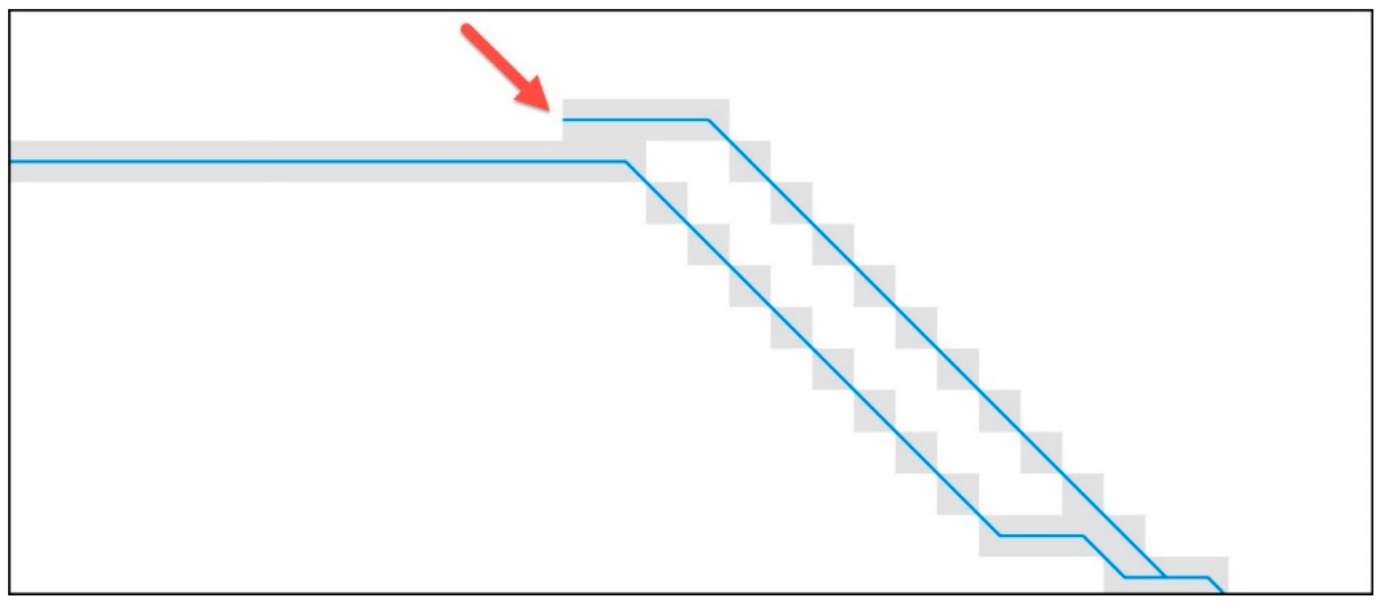
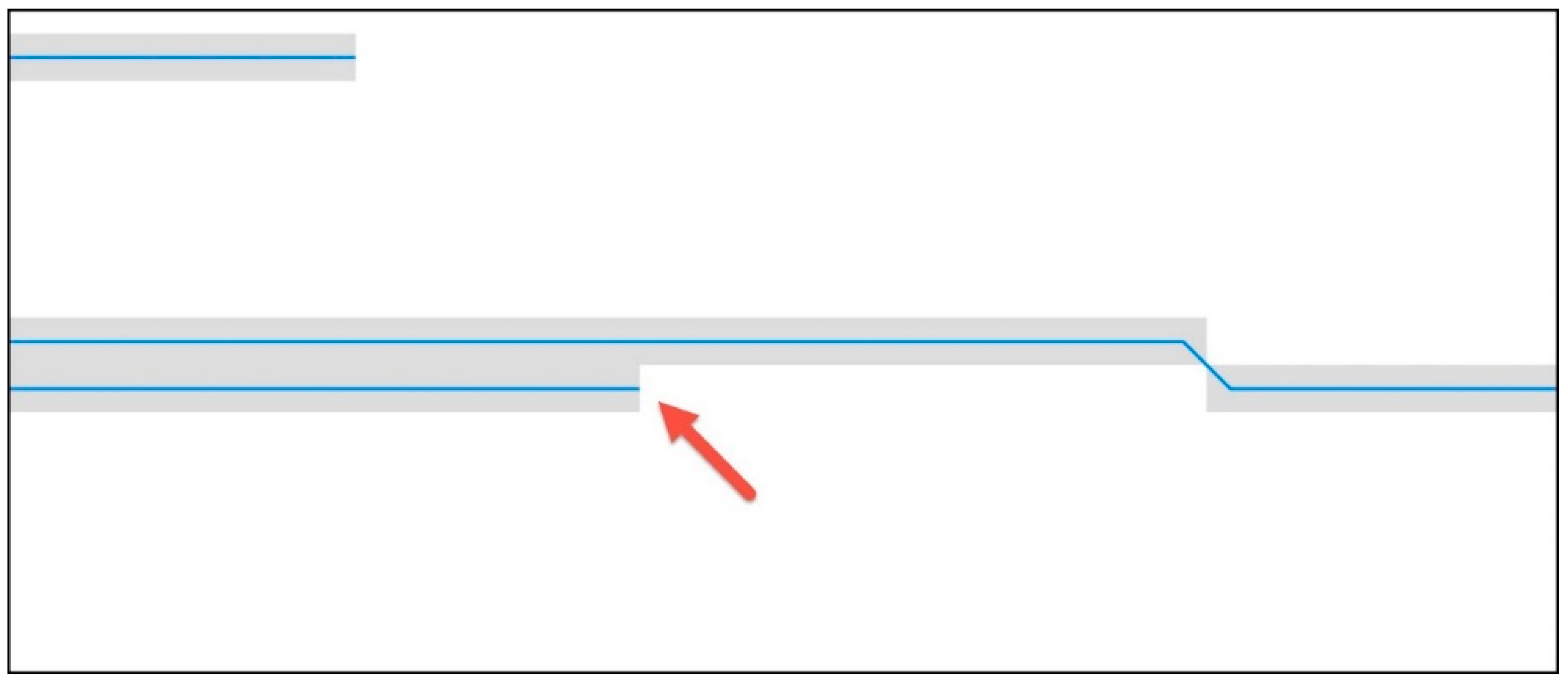
When drainage networks were derived with the stream thresholds determined according to the approaches proposed by Tang [20], Olivera et al. [21], and Heine et al. [24], parallel lines appeared not only in the artificial plains or uniform slopes approaching an inclined plain, but also in other parts of the land. Moreover, some parallel lines were very close to each other. In fact, there were no other cells amongst the cells containing these parallel lines. This suggested that at least one of these lines may be an artificial drainage line as there must be a ridge between the actual drainage lines, even if just a bit. For this reason, among the cells containing parallel lines, there must be other cells in the model to describe that ridge. Here, the BeST and LaST approaches were based on this condition. While this condition is required only at the beginning points of the drainage lines in the BeST approach, it is required from the beginning to the end of the drainage lines in the LaST approach. According to the BeST approach, such a stream threshold must be determined where the cell containing the beginning point of a drainage line is not adjacent to any of the cells containing another drainage line. In Figure 1, the cell containing the beginning point of a drainage line in the place indicated by the arrow mark is adjacent to one of the cells containing another drainage line. There are no other cells between these two cells. For this reason, it is not known whether there is a ridge between them, which is an undesirable situation, according to the BeST approach. According to the LaST approach, a stream threshold must be determined where none of the cells containing a drainage line would be adjacent to none of the cells containing another drainage line. In Figure 2, each of the cells containing a drainage line in the place indicated by the arrow mark is adjacent to one of the cells containing another drainage line. In other words, there are no other cells amongst the cells containing these lines. For this reason, it is an undesirable situation according to the LaST approach.
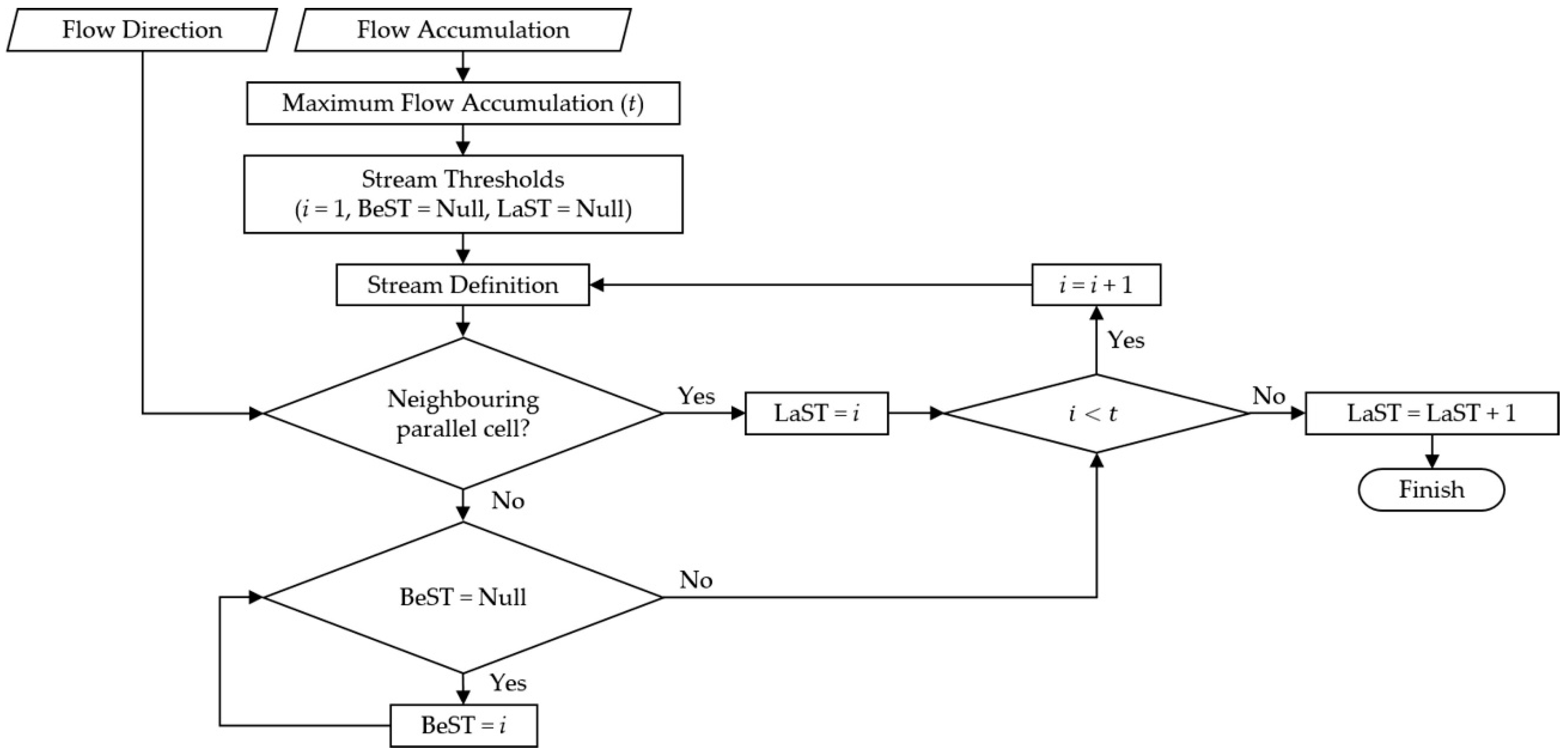
The BeST and LaST values are calculated according to the flowchart in Figure 3 as follows: (1) the value of 1 is set to the stream threshold variable; (2) according to the stream threshold, the stream definition values are determined from the flow accumulation values and thus, drainage lines are also determined; and (3) whether they are “adjacent parallel cells” is checked. Thus, the end of the first iteration is reached. This iteration is repeated each time, increasing the value of the stream threshold variable by 1 up to the maximum flow accumulation value. The BeST condition is provided in the first iteration where adjacent parallel cells are not detected and the LaST condition is provided in the last iteration where adjacent parallel cells are not detected. Consequently, the stream thresholds in the iterations provided by the BeST and the LaST conditions are presented to the user as minimum and maximum stream thresholds.
The flow direction file contains integer values that range from 1 to 255. The values for each direction from the center are 1, 2, 4, 8, 16, 32, 64, and 128. The flow accumulation file contains values determined by accumulating the weight for all cells that flow into each downslope cell. The stream definition file contains values computed based on the flow accumulation values of the cells (that is, if the flow accumulation value of a cell is equal or greater than the stream threshold value, its stream definition value is equal to 1, otherwise, it is −9999).
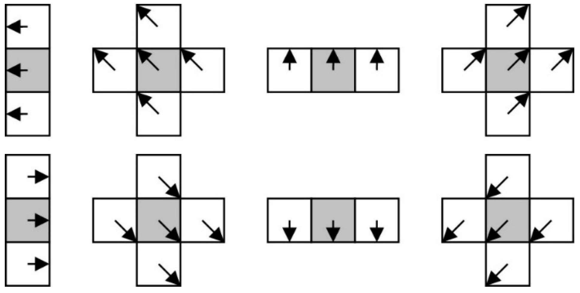
Whether they are “adjacent parallel cells” or not is checked in this way according to their flow direction and stream definition values. All cells with a value of 1 in the stream definition file are examined in turn. If a flow direction value of a cell is 1 or 16, the flow direction values of the cells above and below are checked, respectively; if it is 4 or 64, those on the right and left are checked, respectively; if it is 2, 8, 32, or 128, those above, below, on the right, and on the left are checked, respectively (Figure 4). If the flow direction value of one of the cells checked is the same as the flow direction value of the examined cell, then two cells contain the drainage lines adjacent and parallel to each other. For instance, if the flow direction value of a cell is 1 and the flow direction value of at least one of the adjacent cells above and below is 1, these two cells are adjacent, which means that they contain two drainage lines parallel to each other (Figure 4). Since the cells that appear along the border of the file would not have eight adjacent cells like the others, the limits of the file are extended with one empty cell (the cell with a flow direction value of 0 and a stream definition value −9999). In order for a cell to be a beginning cell of a drainage line, there must be no flow in any of the adjacent cells around that cell.
3. Experiment and Results
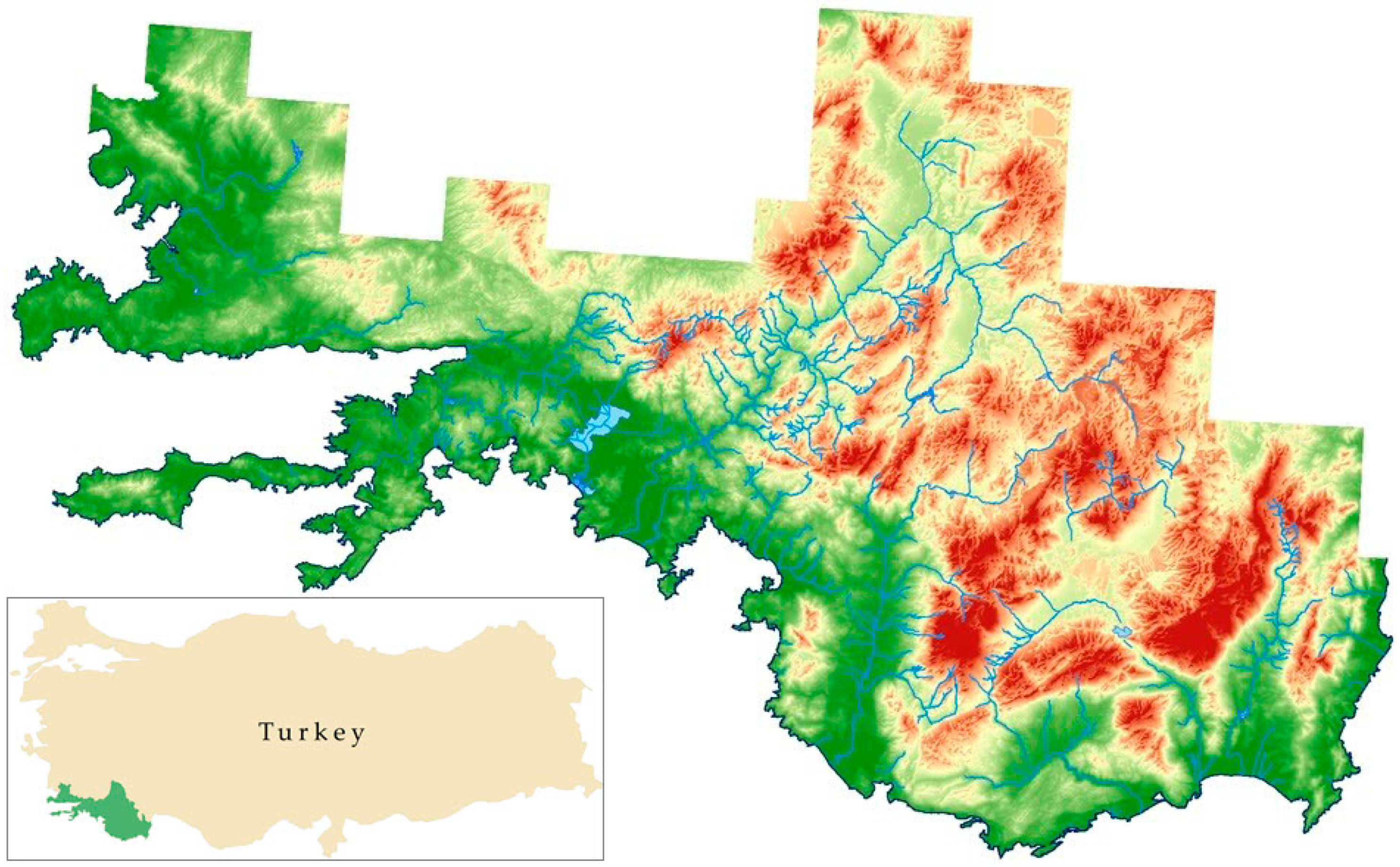
In this study, the elevation (contours and elevation points) and hydrography (streams, channels, lakes, and coastlines) data of 207 databases belonging to the Western Mediterranean Basin produced by the General Command of Mapping were used. The Western Mediterranean Basin is located at the middle latitude zone (between 36.13 and 37.67° latitudes) and east-west elongated (between 27.23 and 30.59° longitudes) and it is a very big basin (approximately 20,554 km2). After data cleaning, a 10 m resolution DEM was obtained by the ArcGIS TopoToRaster tool. Using almost all of the perennial streams, the intermittent streams and channels filling the gaps as well as the middle axes of the related lakes, a largely continuous hydrological network was obtained (Figure 5).
The hydrological network consists of 1001 streams and 36 lake objects in an arc-node data structure. All of the stream objects are steady descending lines in the flow direction and down from the resources. The lake objects are constant elevation polygons. The DEM and flow accumulation statistics are given in Table 1.
The drainage networks were obtained following the below process steps based on the 10 m resolution DEM and the hydrological network using ArcGIS Arc Hydro tools:
- Create Drainage Line Structures
- DEM Reconditioning
- Level DEM
- Sink Evaluation
- Sink Selection
- Create Sink Structures
- Fill Sinks
- Flow Direction
- Adjust Flow Direction in Sinks
- Adjust Flow Direction in Streams
- Flow Accumulation
- Stream Definition
- Stream Segmentation
- Combine Stream Link and Sink Link
- Drainage Line Processing
Since there is a closed sub-basin in the study area, a sink structure was created based on the selected sink which was determined in the sink evaluation process. Therefore, the flow directions in the sink and streams were adjusted.
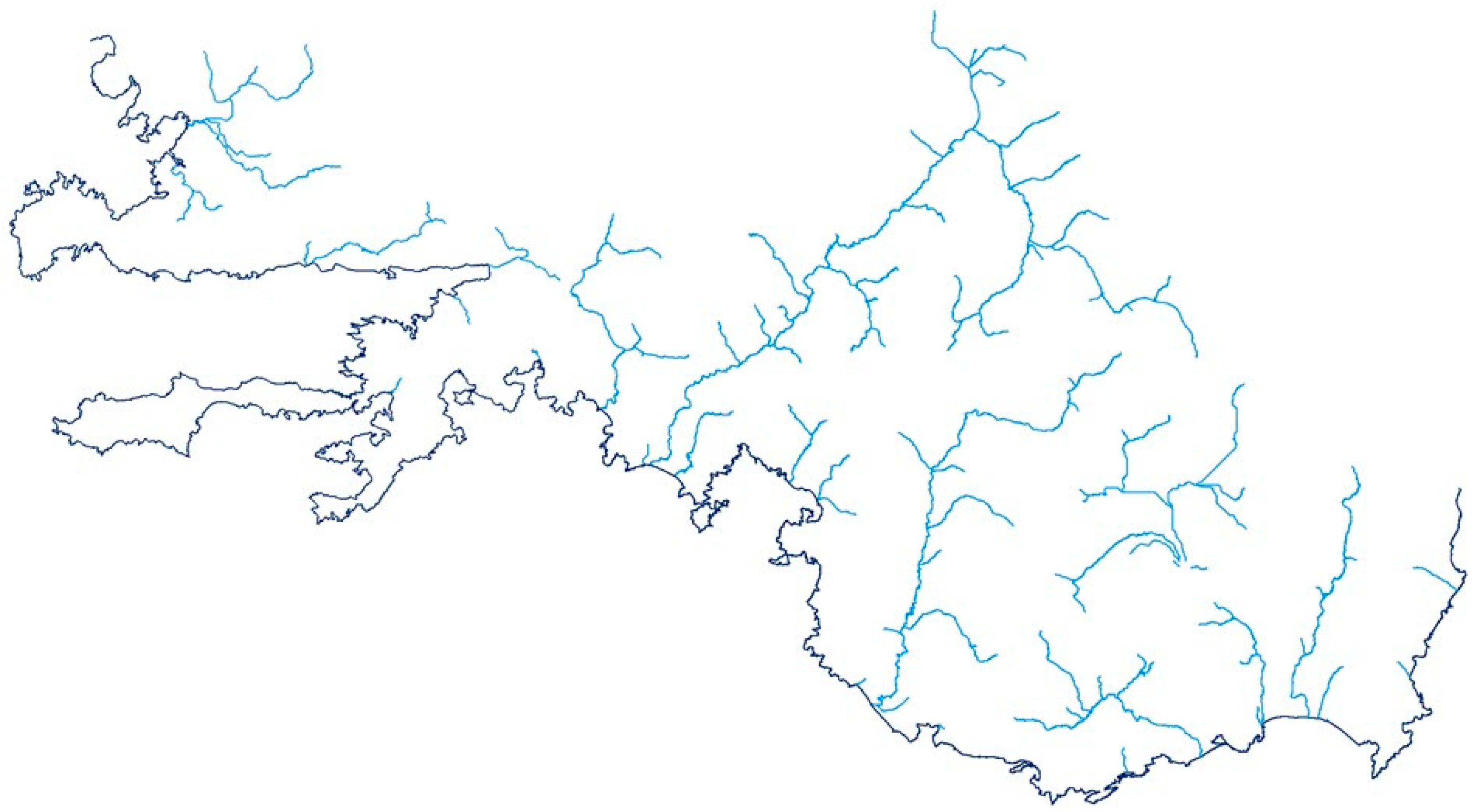
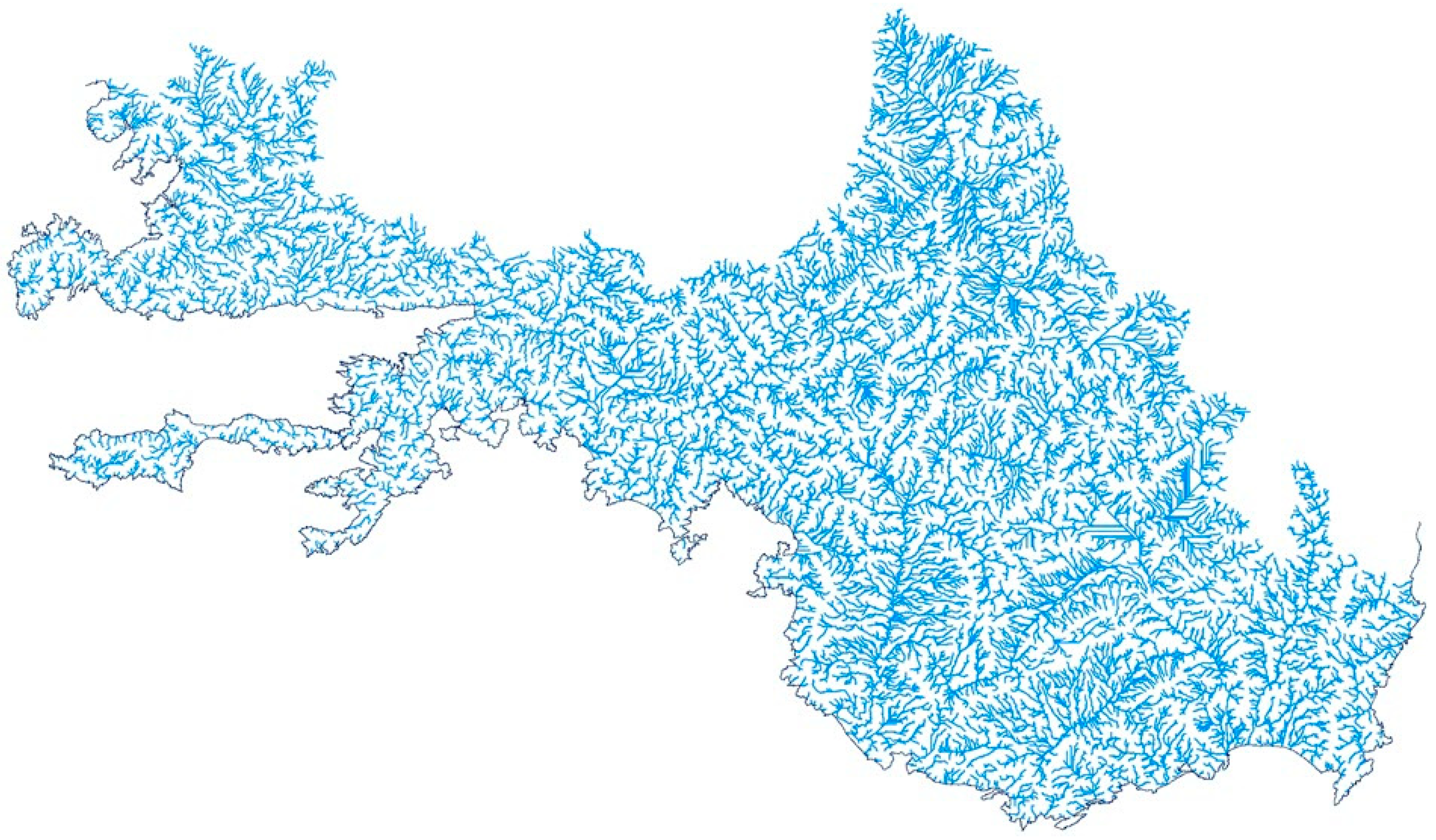
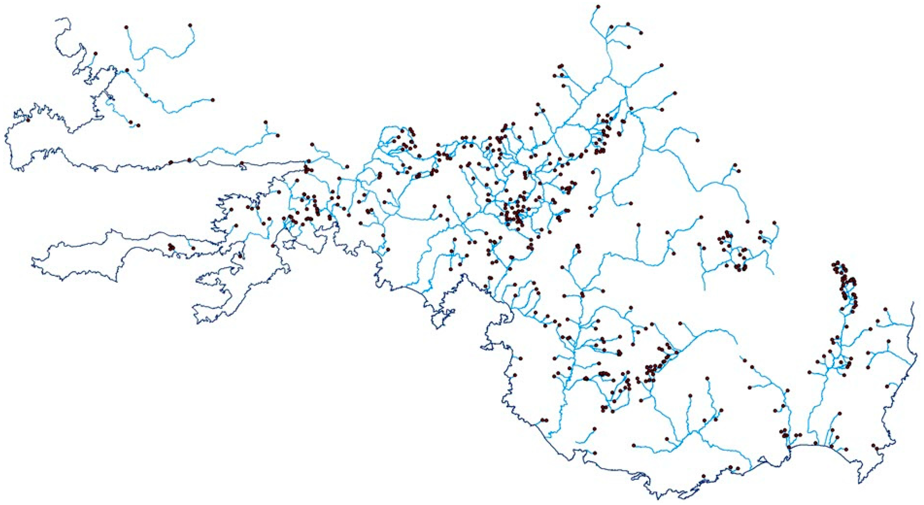
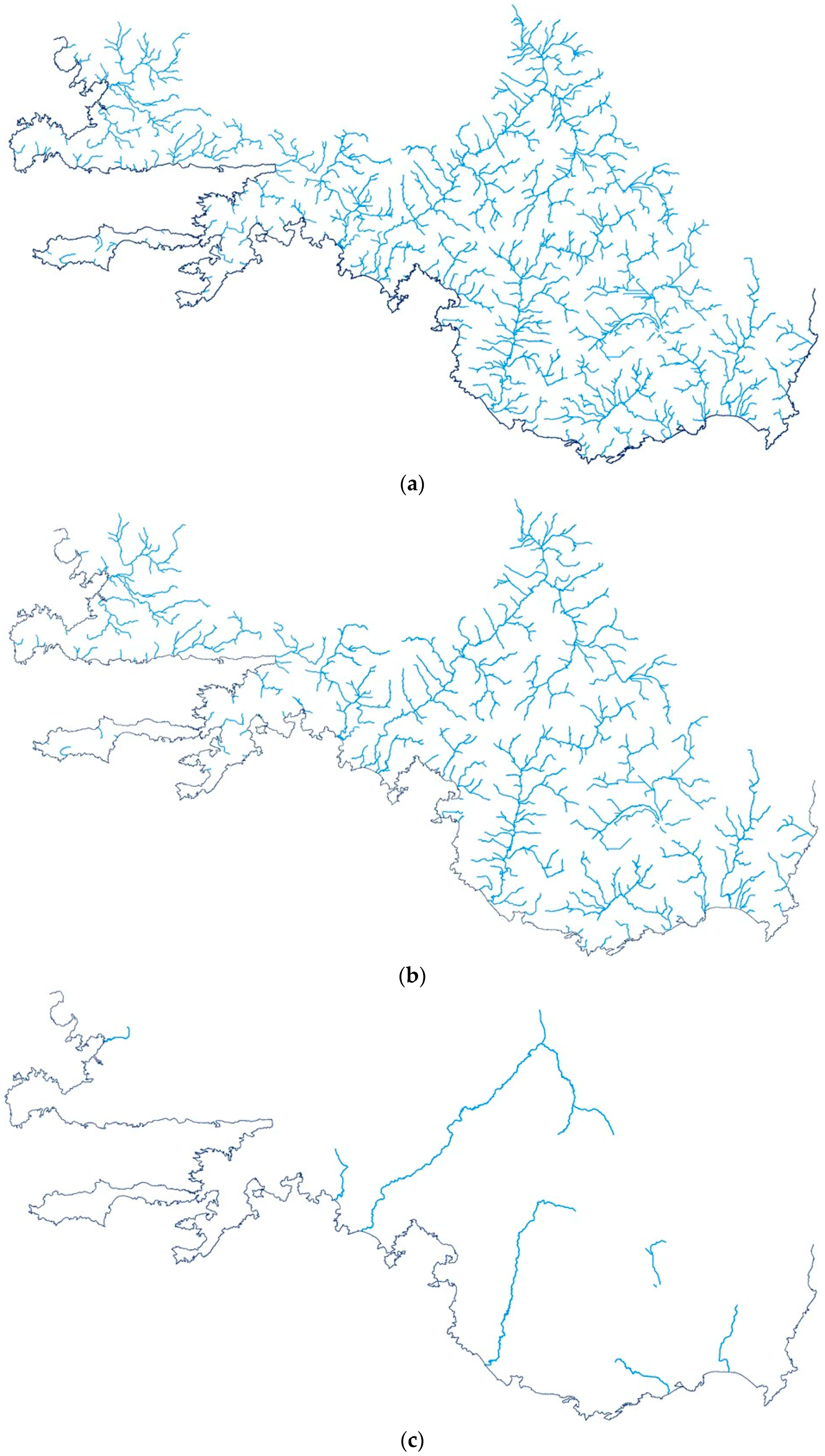
The stream threshold was calculated as 52,692,623 × 0.01 = 526,926, based on the maximum accumulation value, according to the approach proposed by Oliveira et al. [21], to be known briefly as The OnePercent hereafter. The drainage network derived according to this threshold is shown in Figure 6. The mean accumulation value (5765) was used as the stream threshold according to the approach proposed by Tang [20], to be known briefly as the Mean hereafter. The drainage network derived according to this threshold is shown in Figure 7. A total of 538 points on the resources of the tributaries generated the hydrological network to determine the stream threshold according to the approach proposed by Heine [24], to be known briefly as the Heine hereafter, are shown in Figure 8. The arithmetic mean of the flow accumulation values on these points was calculated as 36,541,008/538 = 67,920 and used as the stream threshold. The drainage network derived according to this stream threshold is shown in Figure 9a. The stream thresholds calculated according to the BeST and LaST approaches were 117,622 and 4,974,518, respectively and the drainage networks derived from these values are shown in Figure 9b,c. The BeST and LaST values were computed automatically by a program written in the c# programming language.
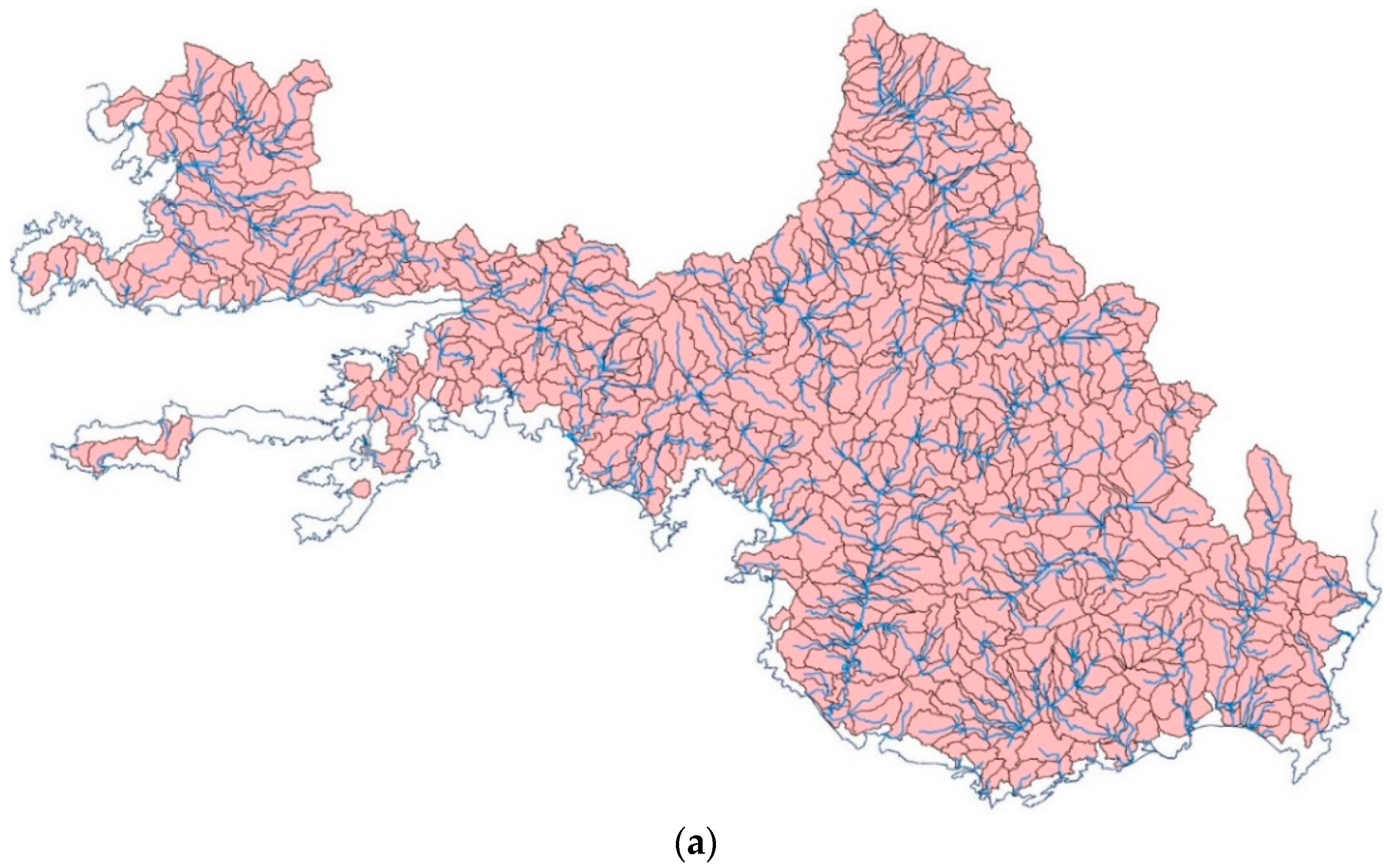
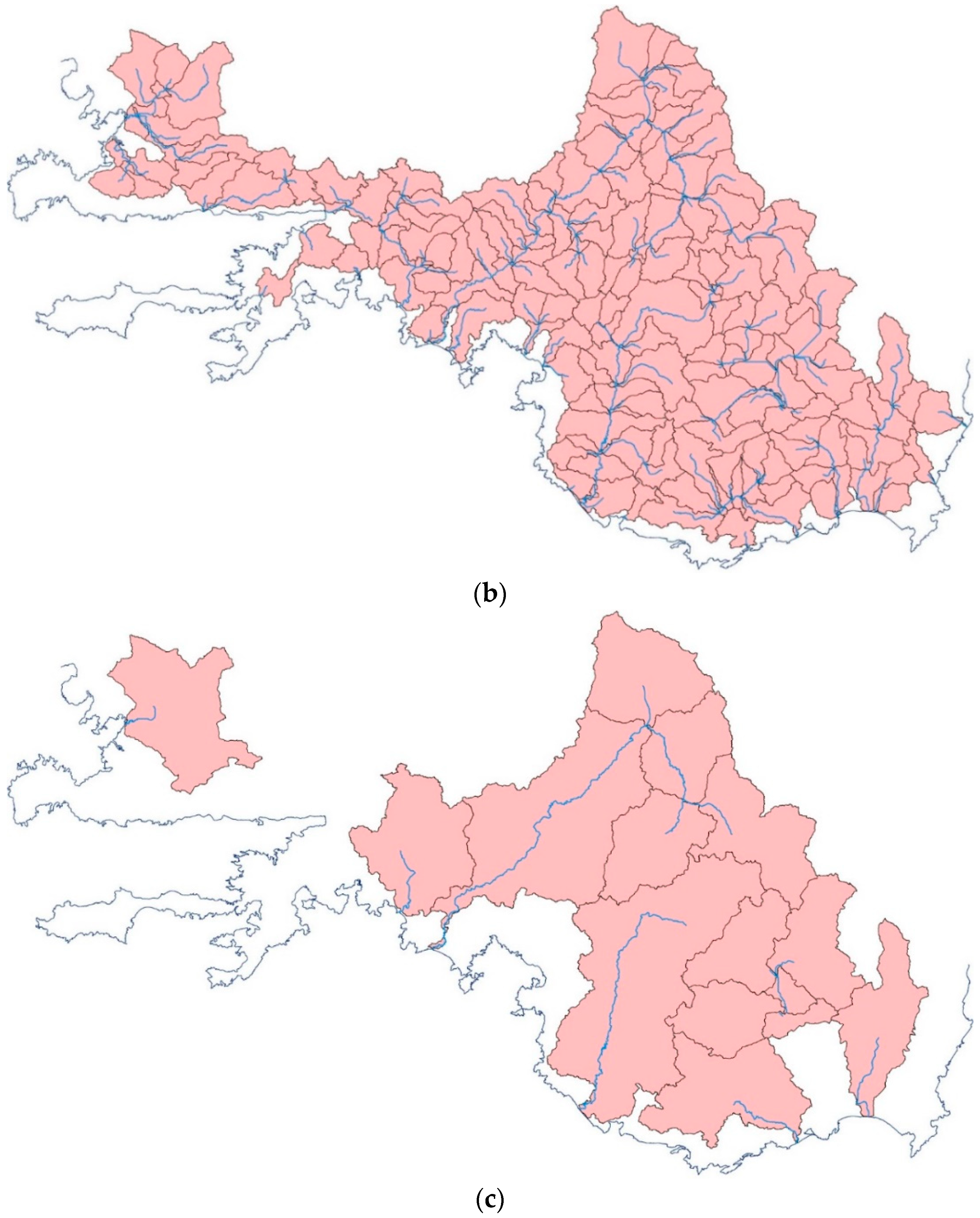
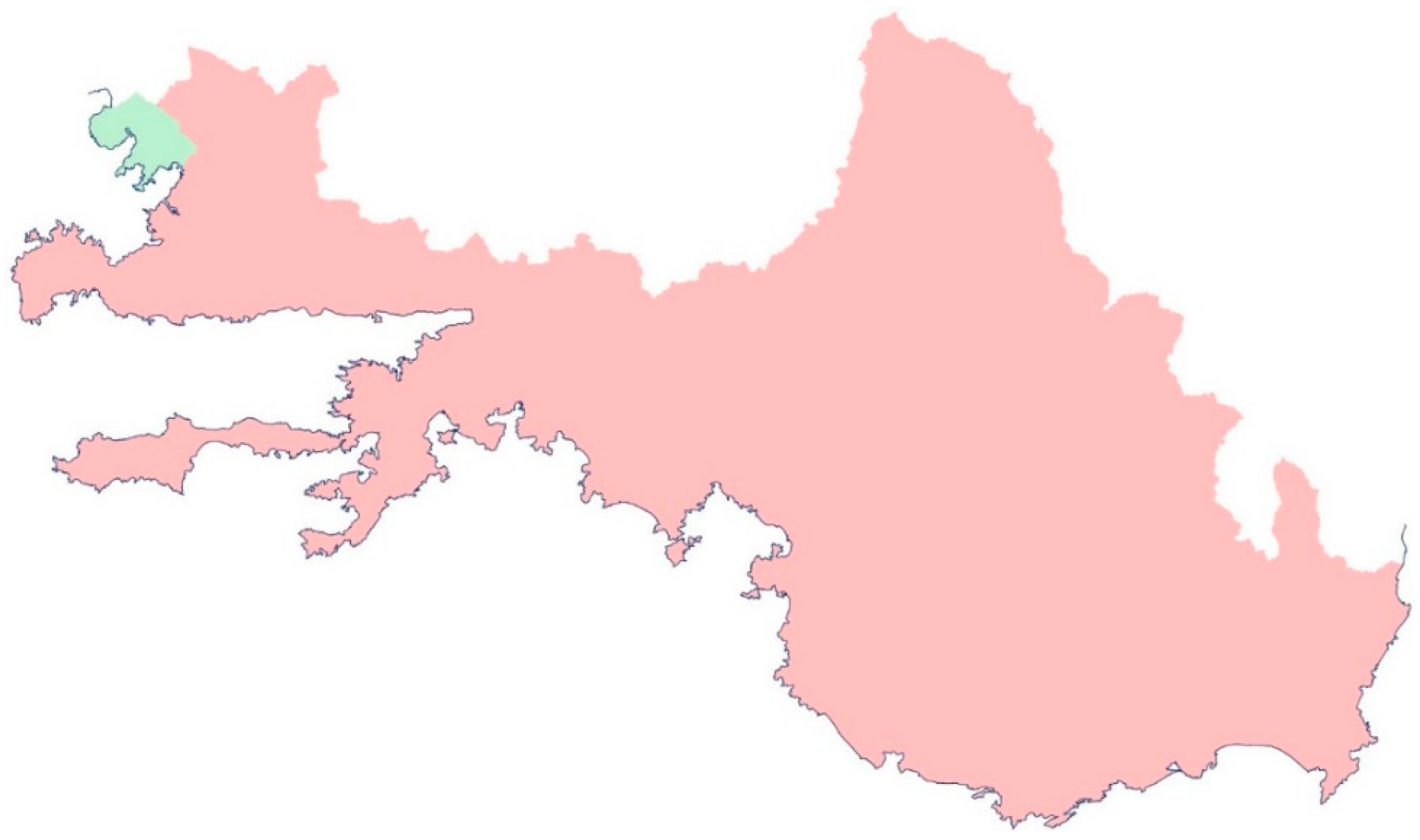
The primary drainage network generated in the first step of the hydrological analysis and the statistics related to the five drainage networks derived according to five distinctive stream thresholds are given in Table 2, collectively. The drainage network closest to the primary drainage network was the drainage network derived by the BeST value. It was understood that there was a negative relationship between the stream threshold and object number and the total length, and a positive relationship between the object number and the total length. Partially or wholly adjacent lines starting from the two adjacent cells in the networks derived according to the Mean and Heine values appeared since the Mean and Heine values were smaller than the BeST value. Furthermore, the OnePercent value was bigger than the BeST value. For this reason, lines that started from adjacent cells in the networks derived according to the OnePercent value did not appear. In addition to that, partial adjacent lines appeared even though they did not start from adjacent cells in the networks derived according to the BeST and OnePercent values since the BeST and OnePercent values were smaller than the LaST value. The catchments derived based on the drainage networks of BeST, OnePercent, and LaST are shown in Figure 10a–c. The numbers of the BeST, OnePercent, and LaST catchments were 891, 187, and 15, respectively. While the Western Mediterranean Basin could be obtained wholly by the BeST catchments, it could only be obtained partially by the OnePercent catchments (missing a first-level sub-basin) (Figure 11). It was also not possible to obtain the Western Mediterranean Basin by the LaST catchments. In conclusion, it can be said that the BeST was the most appropriate value in terms of quality and quantity to be used as the stream threshold in this experiment.
4. Conclusions
The stream threshold is usually determined by a trial and error method by the user depending on the topography of the study area, the DEM resolution, and the purpose of the study (the purpose of using the drainage networks and catchments to be derived). In major hydrological analyses, irrespective of topography and DEM resolution, it is expected that the drainage network to be derived should be at a reasonable level of detail that can reveal all the catchments in the basin. For other purposes, drainage networks at a more or less detailed level may be needed. In this study, a drainage network at a reasonable level of detail was obtained by the BeST value. In this drainage network, there were also no lines starting from two adjacent cells. Drainage networks at a higher level of detail than that required were obtained by the Mean and Heine values. In these drainage networks, parallel lines which started from two adjacent cells and partially or wholly adjacent cells appeared. Drainage networks at a lower level of detail than expected were also obtained by the OnePercent and LaST values. In the network obtained by the OnePercent value, no lines started from two adjacent cells, but there were partially or wholly adjacent parallel lines. In the network obtained by the LaST value, only the main streams in the basin appeared. In this network, there were no parallel lines that started from two adjacent cells nor were there partially or wholly adjacent cells. A drainage network including more or less adjacent lines is not satisfactory in terms of quality and a drainage network which is not able to yield all catchments in the basin is not satisfactory in terms of quantity. Therefore, the knowledge about the adjacent lines can be used in the evaluation of the quality of the drainage network to be derived, and the knowledge about whether all the catchments in the basin will be detected can be used in evaluation of the quantity of the drainage network to be derived. Consequently, the BeST and LaST values provided the user with important clues with respect to the quality and quantity of the drainage network to be derived. The user can estimate that (1) there will be no lines starting from two adjacent cells in the drainage network to be derived by the BeST value (that is, the first clue with respect to the quality of the drainage network to be derived); (2) there will be no wholly adjacent lines in the drainage network to be derived by the LaST value (that is, the second clue with respect to the quality of the drainage network to be derived); (3) all catchments in the basin may not be detected if a value greater than the BeST value is chosen as the stream threshold (that is, the first clue with respect to the quantity of the drainage network to be derived); and (4) only a drainage network generated by major streams can be obtained and all the catchments in the basin may not be detected if a value as great as the LaST value is chosen (that is, the second clue with respect to the quantity of the drainage network to be derived). The Mean, Heine, and OnePercent values did not provide the user with any clues with respect to the quality and quantity of the drainage network to be derived. Finally, we considered that the adjacent parallel line measure was a useful criterion that could be taken into consideration in the stream threshold determination approaches.
Author Contributions
T.G. conceived the study, wrote the paper and interpreted the results. İ.M.O. designed the study, performed the experiments and analysed the data.
Acknowledgments
The authors would like to thank the Scientific and Technological Research Council of Turkey (TUBITAK) for the financial support given under Project No: 115Y411.
Conflicts of Interest
The authors declare no conflict of interest.
References
- Chang, K.T. Introduction to Geographic Information Systems, 3rd ed.; McGraw-Hill: New York, NY, USA, 2006. [Google Scholar]
- Li, Z.; Zhu, C.; Gold, C. Digital Terrain Modeling: Principles and Methodology; CRC Press: New York, NY, USA, 2005. [Google Scholar]
- O’Callaghan, J.F.; Mark, D.M. The Extraction of Drainage Networks from Digital Elevation Data. Comput. Vis. Graph. 1984, 28, 323–344. [Google Scholar] [CrossRef]
- Mark, D.M. Part 4: Mathematical, algorithmic and data structure issues: Automated detection of drainage networks from digital elevation models. Cartogr. Int. J. Geogr. Inf. Geovis. 1984, 21, 168–178. [Google Scholar] [CrossRef]
- Jenson, S.K.; Domingue, J.O. Extracting Topographic Structure from Digital Elevation Data for Geographic Information-System Analysis. Photogramm. Eng. Remote Sens. 1988, 54, 1593–1600. [Google Scholar]
- Gökgöz, T.; Ulugtekin, N.; Basaraner, M.; Gulgen, F.; Dogru, A.O.; Bilgi, S.; Yucel, M.A.; Cetinkaya, S.; Selcuk, M.; Ucar, D. Watershed delineation from grid DEMs in GIS: Effects of drainage lines and resolution. In Proceedings of the 10th International Specialised Conference on Diffuse Pollution and Sustainable Basin Management, Istanbul, Turkey, 18–22 September 2006. [Google Scholar]
- Zhang, W.C.; Fu, C.B.; Yan, X.D. Automatic watershed delineation for a complicated terrain in the Heihe river basin, northwestern China. In Proceedings of the IGARSS 2005: IEEE International Geoscience and Remote Sensing Symposium, Seoul, Korea, 29 July 2005; Volume 1–8, pp. 2347–2350. [Google Scholar]
- Zhou, Q.M.; Liu, X.J. Error assessment of grid-based flow routing algorithms used in hydrological models. Int. J. Geogr. Inf. Sci. 2002, 16, 819–842. [Google Scholar] [CrossRef]
- Costa-Cabral, M.C.; Burges, S.J. Digital Elevation Model Networks (Demon)—A Model of Flow over Hillslopes for Computation of Contributing and Dispersal Areas. Water Resour. Res. 1994, 30, 1681–1692. [Google Scholar] [CrossRef]
- Fairfield, J.; Leymarie, P. Drainage Networks from Grid Digital Elevation Models. Water Resour. Res. 1991, 27, 709–717. [Google Scholar] [CrossRef]
- Garbrecht, J.; Martz, L.W. The assignment of drainage direction over flat surfaces in raster digital elevation models. J. Hydrol. 1997, 193, 204–213. [Google Scholar] [CrossRef]
- Jones, R. Algorithms for using a DEM for mapping catchment areas of stream sediment samples. Comput. Geosci. 2002, 28, 1051–1060. [Google Scholar] [CrossRef]
- Martz, L.W.; Garbrecht, J. An outlet breaching algorithm for the treatment of closed depressions in a raster DEM. Comput. Geosci. 1999, 25, 835–844. [Google Scholar] [CrossRef]
- Tarboton, D.G. A new method for the determination of flow directions and upslope areas in grid digital elevation models. Water Resour. Res. 1997, 33, 309–319. [Google Scholar] [CrossRef]
- Tribe, A. Automated Recognition of Valley Lines and Drainage Networks from Grid Digital Elevation Models—A Review and a New Method. J. Hydrol. 1992, 139, 263–293. [Google Scholar] [CrossRef]
- Turcotte, R.; Fortin, J.P.; Rousseau, A.N.; Massicotte, S.; Villeneuve, J.P. Determination of the drainage structure of a watershed using a digital elevation model and a digital river and lake network. J. Hydrol. 2001, 240, 225–242. [Google Scholar] [CrossRef]
- Gülgen, F.; Gökgöz, T. A New Algorithm for Extraction of Continuous Channel Networks without Problematic Parallels from Hydrologically Corrected Dems. Boletim de Ciências Geodésicas 2010, 16, 20–38. [Google Scholar]
- Tarboton, D.G.; Bras, R.L.; Rodriguez-Iturbe, I. On the Extraction of Channel Networks from Digital Elevation Data. Hydrol. Processes 1991, 5, 81–100. [Google Scholar] [CrossRef]
- Tarboton, D.G.; Ames, D.P. Advances in the mapping of flow networks from digital elevation data. In Bridging the Gap: Meeting the World’s Water and Environmental Resources Challenges; Amer Society of Civil Engineers: Reston, VA, USA, 2001; pp. 1–10. [Google Scholar]
- Tang, G. A Research on the Accuracy of Digital Elevation Models; Science Press: Beijing, China, 2000. [Google Scholar]
- Oliveira, F.; Furnans, J.; Maidment, D.R.; Djokic, D.; Ye, Z. Arc Hydro: GIS for water resources. In Arc Hydro: GIS for Water Resources; Maidment, D.R., Ed.; ESRI, Inc.: Redlands, CA, USA, 2002; Volume 1, pp. 55–86. [Google Scholar]
- Vogt, E.V.; Colombo, R.; Bertolo, F. Deriving drainage networks and catchment boundaries: A new methodology combining digital elevation data and environmental characteristics. Geomorphology 2003, 53, 281–298. [Google Scholar] [CrossRef]
- Lin, W.T.; Chou, W.C.; Lin, C.Y.; Huang, P.H.; Tsai, J.S. Automated suitable drainage network extraction from digital elevation models in Taiwan’s upstream watersheds. Hydrol. Processes 2006, 20, 289–306. [Google Scholar] [CrossRef]
- Heine, R.A.; Lant, C.L.; Sengupta, R.R. Development and comparison of approaches for automated mapping of stream channel networks. Ann. Assoc. Am. Geogr. 2004, 94, 477–490. [Google Scholar] [CrossRef]
- Tantasirin, C.; Nagai, M.; Tipdecho, T.; Tripathi, N.K. Reducing hillslope size in digital elevation models at various scales and the effects on slope gradient estimation. Geocarto Int. 2016, 31, 140–157. [Google Scholar] [CrossRef]
- Romero-Zaliz, R.; Reinoso-Gordo, J.F. An Updated Review on Watershed Algorithms. In Soft Computing for Sustainability Science; Cruz Corona, C., Ed.; Springer: Cham, Switzerland, 2018; pp. 235–258. [Google Scholar]
Figure 1.
An undesirable situation according to the BeST approach: a drainage line starting from a cell adjacent to one of the cells containing an existing drainage line.
Figure 1.
An undesirable situation according to the BeST approach: a drainage line starting from a cell adjacent to one of the cells containing an existing drainage line.

Figure 2.
An undesirable situation according to the LaST approach: a drainage line whose cells are all adjacent to the cells of another drainage line.
Figure 2.
An undesirable situation according to the LaST approach: a drainage line whose cells are all adjacent to the cells of another drainage line.

Figure 3.
The flowchart of the algorithm.

Figure 4.
The eight cases for parallel adjacent cells.

Figure 5.
The DEM (digital elevation model) and hydrological network in the Western Mediterranean Basin.
Figure 5.
The DEM (digital elevation model) and hydrological network in the Western Mediterranean Basin.

Figure 6.
The drainage network derived according to the OnePercent value.

Figure 7.
The drainage network derived according to the Mean value.

Figure 8.
The points on the resources of tributaries that generated the hydrological network.

Figure 9.
(a) The drainage network derived according to the Heine value. (b) The drainage network derived according to the BeST value. (c) The drainage network derived according to the LaST value.
Figure 9.
(a) The drainage network derived according to the Heine value. (b) The drainage network derived according to the BeST value. (c) The drainage network derived according to the LaST value.

Figure 10.
(a) The catchments derived from the BeST drainage network. (b) The catchments derived from the OnePercent drainage network. (c) The catchments derived from the LaST drainage network.
Figure 10.
(a) The catchments derived from the BeST drainage network. (b) The catchments derived from the OnePercent drainage network. (c) The catchments derived from the LaST drainage network.


Figure 11.
The missed first-level sub-basin (green).


Table 1.
The DEM (digital elevation model) and flow accumulation statistics.
| Elevation [m] | Flow Accumulation | |
|---|---|---|
| Minimum | 0.000 | 0 |
| Maximum | 3070.713 | 52,692,623 |
| Mean | 916.181 | 5765 |
| Standard Deviation | 605.676 | 378,405 |
Table 2.
The statistics related to the primary drainage network and the five drainage networks derived according to five distinctive stream thresholds.
Table 2.
The statistics related to the primary drainage network and the five drainage networks derived according to five distinctive stream thresholds.
| Drainage Network | Stream Threshold | Object Num. | Total Length [km] |
|---|---|---|---|
| Primary | 1001 | 3360.082 | |
| Mean | 5765 | 18,444 | 21,599.104 |
| Heine | 67,920 | 1595 | 6113.969 |
| BeST | 117,622 | 891 | 4586.301 |
| OnePercent | 526,926 | 187 | 2011.156 |
| LaST | 4,974,518 | 15 | 551.471 |
© 2018 by the authors. Licensee MDPI, Basel, Switzerland. This article is an open access article distributed under the terms and conditions of the Creative Commons Attribution (CC BY) license (http://creativecommons.org/licenses/by/4.0/).
Share and Cite
MDPI and ACS Style
Ozulu, İ.M.; Gökgöz, T. Examining the Stream Threshold Approaches Used in Hydrologic Analysis. ISPRS Int. J. Geo-Inf. 2018, 7, 201. https://0-doi-org.brum.beds.ac.uk/10.3390/ijgi7060201
AMA Style
Ozulu İM, Gökgöz T. Examining the Stream Threshold Approaches Used in Hydrologic Analysis. ISPRS International Journal of Geo-Information. 2018; 7(6):201. https://0-doi-org.brum.beds.ac.uk/10.3390/ijgi7060201
Chicago/Turabian StyleOzulu, İbrahim Murat, and Türkay Gökgöz. 2018. "Examining the Stream Threshold Approaches Used in Hydrologic Analysis" ISPRS International Journal of Geo-Information 7, no. 6: 201. https://0-doi-org.brum.beds.ac.uk/10.3390/ijgi7060201
Note that from the first issue of 2016, this journal uses article numbers instead of page numbers. See further details here.