Analyzing Space-Time Dynamics of Theft Rates Using Exchange Mobility

1
State Key Lab of Information Engineering in Surveying Mapping and Remote Sensing, Wuhan University, Wuhan 430079, China
2
Collaborative Innovation Center of Geospatial Technology, Wuhan 430079, China
3
Key Laboratory of Aerospace Information Security and Trusted Computing of the Ministry of Education, Wuhan University, Wuhan 430079, China
4
De Key Laboratory of Police Geographic Information Technology, Ministry of Public Security, Changzhou 213022, China
5
School of Geographical Sciences and Planning, Guangxi Teachers Education University, Nanning 530001, China
6
Education Ministry Key Laboratory of Environment Evolution and Resources Utilization in Beibu Bay, Guangxi Teachers Education University, Nanning 530001, China
7
Department of Sociology, Kent State University, Kent, OH 44240, USA
*
Authors to whom correspondence should be addressed.
ISPRS Int. J. Geo-Inf. 2018, 7(6), 210; https://0-doi-org.brum.beds.ac.uk/10.3390/ijgi7060210
Submission received: 1 May 2018
/
Revised: 21 May 2018
/
Accepted: 27 May 2018
/
Published: 2 June 2018
Abstract
:A critical issue in the geography of crime is the quantitative analysis of the spatial distribution of crimes which usually changes over time. In this paper, we use the concept of exchange mobility across different time periods to determine the spatial distribution of the theft rate in the city of Wuhan, China, in 2016. To this end, we use a newly-developed spatial dynamic indicator, the Local Indicator of Mobility Association (LIMA), which can detect differences in the spatial distribution of theft rate rankings over time from a distributional dynamics perspective. Our results provide a scientific reference for the evaluation of the effects of crime prevention efforts and offer a decision-making tool to enhance the application of temporal and spatial analytical methods.
1. Introduction
To understand the geography of crime it is necessary to determine the differences in the spatial distribution of the criminal phenomenon. Numerous studies have focused on determining such spatial distribution patterns by detecting hot spots or calculating spatial autocorrelation [1,2,3,4,5,6,7]. Well-known methods exist for incorporating spatial autocorrelation or detecting hot spots, such as eigenvector spatial filtering (ESF) [8,9,10,11,12] and space-time scanning statistics [13,14,15,16,17,18,19]. However, both these methods are static approaches that detect the differences between geographical units over a specific time range, therefore failing to account for the fact that such a distribution usually changes over time and neglecting temporal and spatial evolutionary patterns. Other researchers have investigated time variations in crime distribution, especially regarding monthly or seasonal changes in crime based on routine activity theory [20]. The differences between two periods in the distribution of crime events are often interpreted as a characteristic of cross-sectional data for a specific time [21,22,23]. For example, Breetzke and Cohn [21] evaluated monthly differences in assault levels stratified by neighborhood and found assault to be seasonal, with higher incidence rates in summer. In other words, they generalized the periodicity of crime distribution. While this is valuable, it is difficult to determine how to numerically describe the changes in the spatial distribution pattern between different periods, and thus, this is often ignored.
Although spatial dynamics have been found to be widespread in science and widely used across a variety of disciplines, especially in economic issues [24,25,26], their application to crime analysis is still limited. However, determining a method for measuring the changes in the economic levels of individuals in a group relative to the changes of other individuals in the group over a period is a crucial issue in economics [27,28,29]. Different types of changes in the distribution patterns of individual economic levels indicate different social welfare states [30]. In other words, the spatial differences described by traditional spatial-temporal statistics do not consider positive or negative effects on economic inequality due to economic mobility. Similar to the problem above, when the spatial heterogeneity of crime events certainly exists, it is unclear whether criminal incidents always concentrate in a few geographical units in a study area or switch between most of the geographical units. To understand the importance of analyzing changes in the spatial distribution of crime over time, assume there are two geographical spaces, i and j, in which 100 and 10 crimes were respectively committed over a specific month. To understand the change in crime over time, we need to consider the following two possibilities:
- (1)
- In the second month, i will witness 10 crimes and j will witness 100 crimes. If investigating two different periods, the spatial distribution of crimes may greatly differ in each period. However, there is the probability that there will be an overall similar number of crimes, because exchange mobility exists between i and j and, therefore, there ought to be a similar overall amount of crime. However, these two-time periods cannot be combined, even though it appears that both areas have similar numbers of crimes, since we ignore differences over time.
- (2)
- In the second month, the distribution of crimes remains the same: 100 in i and 10 in j. In this case, it is important to note that i always has a higher rate of crime than j. Similar to the significance of consolidation of income levels in socioeconomic processes [8,9,10,11], the consolidation of the theft rate level also needs to be noticed—in this situation the differences between i and j must be emphasized.
In this paper, we use the concept of exchange mobility (also known as space-time coherence from the perspective of calculation) to better understand the spatial distribution of theft cases at the community level in Wuhan City, China. To do so, we use a newly-developed spatial dynamics indicator, called the Local Indicator of Mobility Association (LIMA) [31], which is based on Kendall’s statistic. Unlike traditional spatial autocorrelation or spatial-time statistics, LIMA measures changes in the rank of crime level in a specific geographical unit over different periods and compares these changes to those in an adjacent geographical space. In other words, LIMA statistics are designed to detect hot-spots of space-time concordance and to determine change patterns in spatial pattern evolution, as demonstrated in the two examples above.
We use Wuhan’s districts as our spatial divisions. This allows us to consider the stability of the spatial and temporal distributions of theft rates in all communities, among and within districts, through the exchange mobility of the rank of crime rates among communities. This paper focuses on theft, a criminal type of multiple property conversion with a low detection rate. Public security at all levels is closely concerned with the prevention and control of this type of crime. In addition to the accumulation of theft over time and space, theft is also a good example of a type of crime that shows mobility, which will be explored in the following section. The rest of this paper is structured as follows: the remainder of the Introduction reviews the relevant literature. Section 2 describes the research methods and data used in this paper, Section 3 provides an overview of our results, and Section 4 offers a discussion of our research and some conclusions.
Spatial autocorrelation is an important property of geographical data and one of the major differences between spatial statistics and traditional statistics [4,5,6,32] or measurement that model spatial autocorrelation [8,10,11]. It describes the difference between geographic variables related to locations in the geographical space domain and the same variables in spatial-adjacent locations. Cliff et al.’s (1973) definition of spatial autocorrelation and Tobler’s proposed first law of geography were milestones in the field, and provided effective measures of statistical significance to allow the establishment of relationships between quantifiable spatial data [4].
Spatial autocorrelation pertains to the non-random pattern of attribute values over a set of spatial units. It has been used to understand crime rates in a variety of ways, including traditional geographical statistics (e.g., Moran’s I). For instance, Malleson and Andresen studied the relationship between social networks and crime, analyzing the spatial differences between disease and crime based on Moran’s I [33]. However, traditional autocorrelation statistics represent only snapshots related to the distribution of spatial variables in the study area within a period of time. Their findings are static and lack a description of the development of spatial variables over time.
Another related literature stream is the spatiotemporal analysis of crime, including methods such as space-time scanning statistics or time series analysis [13,14,15,16,17,18,19]. The main idea of space-time scanning statistics (STSS) is to scan the data in the study area along the time and space dimensions through the spatiotemporal window with changes in position and size, where each window is seen as a potential anomaly space-time gathering area. The results of STSS are one or more space-time windows, representing the most aggregated areas of events over space and time. However, the pattern of crime distribution between two time periods has not drawn much attention, while time series analysis attracted the attention of crime geographers. For example, Melo [20] analyzed spatial patterns using census tracts and temporal patterns, considering time variance (seasons, months, days, and hours) based on routine activity theory, and found the distribution patterns of different crime types to present different time variances when changing temporal or spatial/temporal scales. Breetzke [21,22] analyzed time variation (monthly and daily) for violent and property crimes based on Fourier analysis and found the periodicity of crime to be around 7–10 days. Schinasi [23] conducted a time series analysis on the associations between temperature and crimes based on a quasi-Poisson distribution. The analyses suggested that the risk of violent crimes is highest when temperatures are comfortable, especially during cold months. In other words, they generalized the periodicity of crime distribution. While this is valuable, the problem is how to numerically describe the changes in spatial distribution patterns between different periods, which is often ignored. As the time variation analysis of crime more closely follows the idea presented by LIMA, we focus on how to numerically describe the changes in the spatial distribution patterns between different periods.
In contrast to the testing-based methods mentioned above, other papers have focused on model-based methods for space-time modeling to describe the spatial differences in geographic space. These are usually modeled with generalized linear mixed models based on eigenvector spatial filtering (ESF) [8,9,10,11,12] or Bayesian approaches [34,35,36,37,38,39]. ESF is a nonparametric statistical method for modeling spatial autocorrelation in the context of linear and generalized linear or geographic weighted regressions [8,9,10,11,12]. In a generalized linear mixed model, the eigenvectors can be used to capture the spatial autocorrelation in residuals and, hence, the estimation of a standard linear regression model does not suffer from a violation of the independence assumption due to spatial autocorrelation. For example, Chun [10] illustrated how ESF can be utilized to model space-time crime data, extending the generalized linear mixed model for space-time vehicle burglary incidents in the city of Plano, Texas. ESF introduces a subset of eigenvectors extracted from a spatial weights matrix as synthetic control variables in a regression model specification to deal with the problems involving spatial dependences in a spatial regression model. In other words, it accounts for spatial autocorrelation in the standard specifications of regression models.
Other papers have focused on Bayesian approaches. For example, Jane Law [34] used a spatial-temporal Bayesian modeling method to analyze the changes in the incidence of property crime in York city, Canada, estimating linear (mean) and non-linear (area-specific differential) trends in property crime. Wheeler [35] used a Bayesian model for the estimation of the spatially-varying effects of alcohol outlets and illegal drug activity on violent crime in Houston. Enrique et al. [36] analyzed the variation in violent crimes by area and its association with neighborhood-level explanatory variables using a Bayesian spatial random-effects modeling approach. They showed that areas with high levels of violent crime are more likely to be those with a high immigrant concentration, public disorder and crime, and high physical disorder. Several recent papers have also examined the contextual influences on juvenile offenders and violent crime using a Bayesian spatial modeling approach [37,38]. In general, the Bayesian spatiotemporal model is developed from traditional spatial regression models, such as the spatial lag model and the spatial error model. The goal of the Bayesian spatiotemporal model is to measure the influence of a specific geographical variable or explanatory variable (e.g., house value, education, poverty, unemployment, vehicle, working at home) on the crime rate level, and then, to predict the crime tendency level. The Bayesian spatiotemporal model adds to the understanding of the relationship between criminal risk and neighborhood characteristics. In other words, this model is concerned with the characteristics of spatial distribution rather than the degree of change in spatial distribution.
LIMA is designed to deal with the problem described above [31,40] and can be viewed as a ramification of the local indicators of spatial association (LISA), suggested by Anselin [3]. It originated from the ideal that existing spatial-time statistic deficiencies in the description about economic inequality are inadequate to describe a study area’s regional differences, simply by using traditional statistics based on cross-section data, such as space-time or spatial autocorrelation [40,41,42,43,44]. Different forms of LIMA are suggested as alternative representations of regional contexts [31]. LIMA measures consider how pairwise ordinal associations between neighboring values evolve over time, while differences between the spatial autocorrelation or spatial-time statistics capture how pairwise interval associations change between time periods. The two measures (LISA and LIMA) should be thought of as complements and not substitutes because they capture different aspects of spatial distribution dynamics.
In summary, this paper relies on two concepts from previous research. First, exchange mobility (or space-time concordance) measures how pairwise ordinal associations between neighboring values evolve over time. Second, the intraregional exchange mobility of each district and interregional exchange mobility between districts are analyzed by decomposition with of LIMA. By measuring the exchange mobility of the theft rate ranking, a dynamic perspective can be formed as a useful complement to the space autocorrelation measure, to overcome the deficiency that traditional spatiotemporal analysis methods based on cross-sectional data cannot address—the numerical changes in the spatial pattern evolution of crime events.
2. Materials and Methods
2.1. Study Area
We conducted our study in the city of Wuhan, Hubei Province, China (Figure 1). Wuhan is a megacity that serves as the political, economic, and educational center of central China. Yangtze River, the third largest river in the world, divides Wuhan’s downtown into three parts, and Han River, its largest tributary, divides the three main towns (Wuchang, Hankou, and Hanyang). Wuhan has 13 municipal districts and 160 sub-districts [45]. The city has a total area of 8494.41 km2, and the downtown area is 863 km2. The permanent population is about 10.7662 million.
The development of a police information system in Wuhan and the application of a police GIS resulted in the accumulation of a large amount of crime data. The use of administrative divisions (districts) or the institutional arrangement of the national structural system through spatiality and hierarchy is necessary for certain administrative functions. Different districts have different areas of focus, such as politics, economics, nationality, population, geography, and culture. Due to the complexity of urban management and the limitations of human management, the city must be managed through an administrative management system based on the division of labor and hierarchical control.
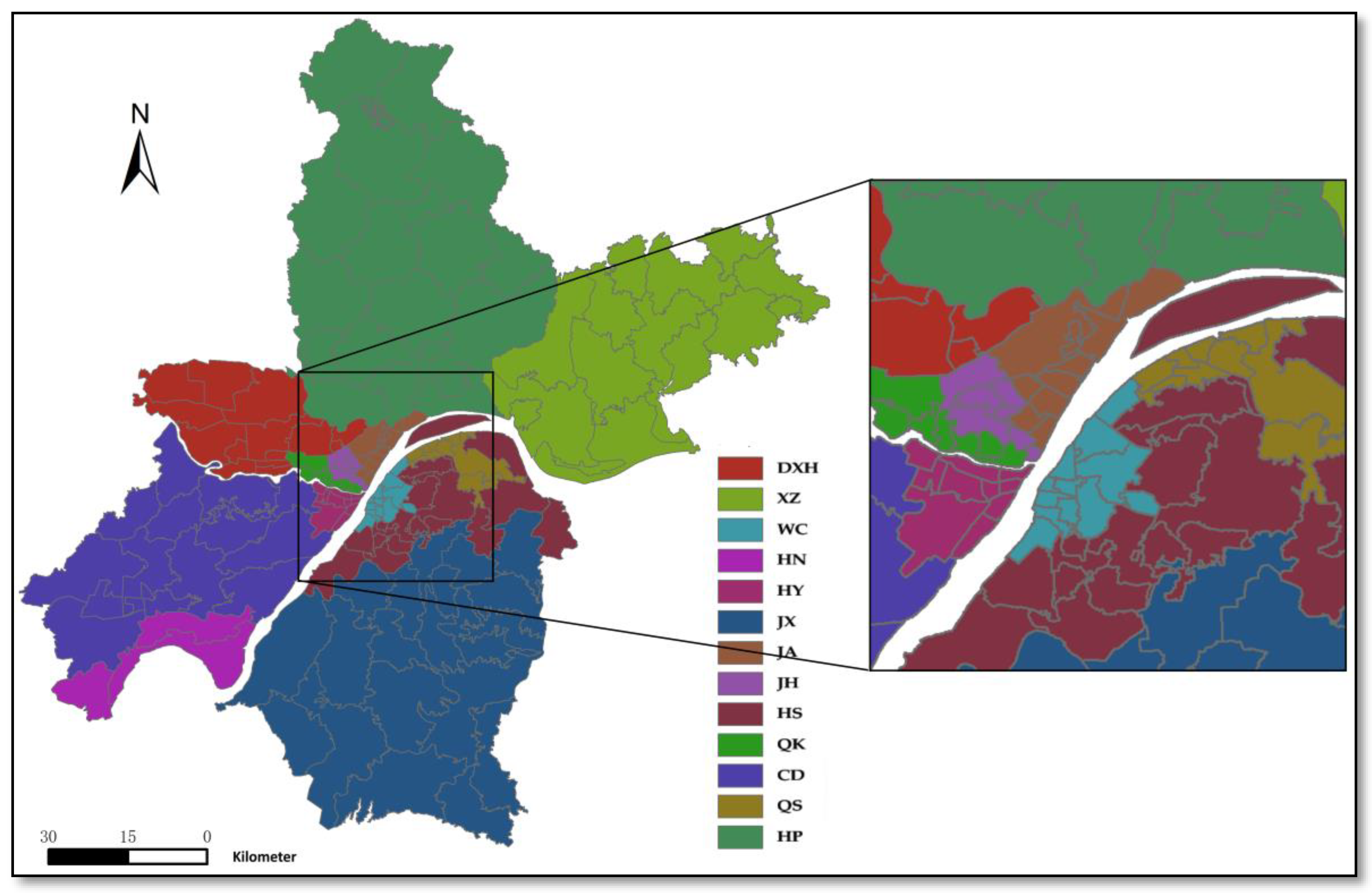
Wuhan include seven downtown districts (Jiang’an (JA), Jianghan (JH), Qiaokou (QK), Hanyang (HY), Wuchang (WC), Qingshan (QS), and Hongshan (HS)) and six suburban districts (Caidian (CD), Jiangxia (JX), Huangpi (HP), Xinzhou (XZ), Dongxihu (DXH), and Hannan (HN)) (Figure 2). Each has different characteristics; for example, most colleges and universities in Wuhan are concentrated in Wuchang, while commercial and political centers are concentrated in Jianghan and Qiaokou. Meanwhile, Caidian and Dongxihu have many scenic spots, meaning that the tourism industry is relatively developed in both districts, and industries are concentrated in Hanyang, Xinzhou, and Qingshan.
This paper defines the spatially close relationships between various communities from a district perspective. We use LIMA’s decomposition forms to analyze the differences within and between the temporal and spatial distribution of the theft rate ranking in all districts.
2.2. Dataset
The data in this paper come from the Police Geographic Information System (PGIS) system of Wuhan’s Public Security Bureau. We analyzed all cases of theft for the 12 months between 1 January 2016 and 31 December 2016, for a total of 148,995 incidents. Each record included the case type, occurrence time (accurate to the day), location (geographical coordinates), case description, and other properties. Additionally, the data used to support the temporal and spatial hotspot analysis of criminal cases included division data of urban districts and 2013 population data for all 9,896,726 inhabitants (due to the sensitivity of data, we only have the census data for 2013.). Each population record included personal IDs and addresses (geographical coordinates). Table 1 summarizes the data used in this paper.
Figure 3 shows the distribution of theft rates using theft data as a whole for 2016 (Quarter 1 lasted from January to April), population data for 2013, and vector data of the districts in Wuhan.
2.3. Methods
2.3.1. Rank Correlation
Kendall’s [46] is based on the comparison between the number of observation pairs that have concordant ranks between two variables [47]. Kendall’s coefficient is used to express the degree of similarity between two variables; for example, it can be used as the distance measure in rank aggregation problems on pattern recognition and machine learning [48,49,50,51,52,53,54] or it can measure rank correlation in change detection [55,56] in the spatial sciences and the more general problem of map comparisons [57,58] and their fast algorithms [47,59,60].
Kendall’s τ is a nonparametric statistical method that measures the degree of similarity between two rankings (ordinal variables) and can be used to assess the significance of the relationship between them. Nonparametric statistics differ from parametric statistics in that the model structure is not specified a priori but is instead determined from the data. The prerequisite for a parametric statistical method is that the data should obey or approximate the normal distribution, whereas nonparametric statistical methods do not rely on any assumptions on distributions, which is more suitable for geographic random variables.
To measure the spatial dynamics of crime distribution, we used one attribute measured at two points in time over spatial units as our two variables. This classic measure of rank correlation indicates the relative stability in the map pattern over the two periods and can be formulized as follows (Equation (1)):
where f and g are variables with observations over units. The numerator reflects the net concordance between all pairs of observations with these two variables, where c is the number of concordant pairs and d is the number of discordant pairs. Any pair of observations or , where is said to be concordant if the ranks for both elements (more precisely, the sort order) by and by agree, that is, if both and or if both and . They are said to be discordant if and or if and . If or , the pair is neither concordant nor discordant. As a correlation measure, the range is .
2.3.2. Local Crime Exchange Mobility
There are numerous mathematical models that describe exchange mobility [25,40], and one of the most common of these is a series of measure methods based on the development of Kendall’s correlation coefficient [24]. The LIMA is based on Kendall’s correlation and stems from the consideration of the question about regional income inequality [31,40], on which Rey has done significant research [31,40,59,60,61].
Although the temporal and spatial patterns for different periods can also be demonstrated with spatial autocorrelation statistics through changes in autocorrelation measures over time, their differences are significant. LIMA describes differences in spatial patterns during evolution in the way that spatial patterns jointly form—with the evolution of geographical units and their neighbors—while local autocorrelation statistics describe the differences between geographic variables of a geographical unit and its neighborhood at a time point. The LIMA [31,41] formula is as follows:
where is the focal unit and is one of its geographical neighboring pairs; is the spatial weight (let denote a binary spatial weights matrix with elements if observations r and b are geographical neighbors, and 0 otherwise); (c is the number of concordant pairs and d of discordant pairs); ; and is the geographic weight indicating the importance of r to b, which is determined by geographic weight.
LIMA compares the local concordance measure for each neighbor against the same measure for the focal unit, and the concordance between neighboring pairs of the focal unit is also considered to integrally describe how the focal unit’s spatial pattern of rank changes. In other words, in addition to the concordance relationships between the focal unit and its neighbors, the concordance between all the pairs within the focal unit’s neighborhood set are also included. The LIMA value for a certain geographical unit represents the change in local rank in the adjacent geographical space at the site between two time periods (e.g., from Q1 to Q2 in this paper). The statistics on the quantity of all geographical units in the geographical space in relation to the local ranks of the two periods are obtained.
Here, the question is whether the concordance relationship between the focal community and its neighbors is different from what could be expected from randomly distributed rank changes. Because the assumption of equal distance between categories does not hold for ordinal data, neither the use of means and standard deviations for the description of ordinal distributions, nor the use of inferential statistics based on means and standard deviations were appropriate. Instead, nonparametric methods were proposed as the most appropriate procedures for inferential statistics involving ordinal data, especially those developed for the analysis of ranked measurements. We performed a Monte Carlo simulation to determine the statistical significance of the results [31] and the statistics were computed under the null hypothesis of random spatial patterning of rank changes [31]. Inference was based on conditional randomization for each community under the null hypothesis. That is, the sampling distribution for the focus community was obtained by randomly selecting its neighbors from the set of communities in Wuhan, excluding itself and recalculating the statistic. Permutation re-sampling requires a computationally demanding number of permutations to get reliable estimates of the p-values for the most differentially expressed genes. This process was repeated 99 times for each state and pseudo p-values were obtained by comparing the observed statistics to this conditional distribution under the null hypothesis.
2.3.3. Decomposition of Crime Exchange Mobility
The occurrence of crime has profound and complex roots, including numerous societal, economic, cultural, and spatial factors. Hence, differences often exist in the spatial distribution of criminal incidents. The definition of a spatial neighborhood in a traditional geographical statistical analysis is often based on proximity in the geographical space. However, this convention has some limitations, especially in cities in developing countries, where the distribution of resources (e.g., manpower, economic, police) is highly unequal. Although the communities subordinate to different districts are geographically close, there may be widely divergent administrative means and efficiencies. Therefore, it is unreasonable to compare their subsets. There is a government for each city, but there are also a number of decision-making centers at the district level. The differences among district governments, jurisdictional districts, and districts (the smallest administrative units in China) are objective facts, and our methods must take these differences into account.
The decomposition of exchange mobility proposed by Rey et al. [31] measures intraregional and interregional mobility using block weights that partition spatial observations into regimes and facilitate the decomposition of overall mobility into two components in a given study area. This interregional and intraregional mobility decomposition is calculated as follows:
where and is a unit vector; P is the regional aggregation matrix of dimension with being equal to the number of regions. The matrix is defined with elements if observations are concordant, if if they are discordant, and otherwise. This defines a fast algorithm for the Kendall’s . Using this aggregation matrix, the local concordance measures can be aggregated to consider the concordance between and within regions. This is used to exhaustively and mutually exclusively partition the areas into K regions, such that if , otherwise , and . This can be shown in matrix form as
where is a concordance matrix with the diagonal elements measuring the concordance between units within a regime and the off-diagonal elements denoting the concordance between observations from a specific pair of different regimes.
The decomposition determines whether the classic measure masks different correlation patterns between the two pair sets: neighboring and non-neighboring. The first term on the right-hand side of Equation (3) is a function of intraregional concordance, while the second is driven by the concordance between members of different regions, or interregional concordance. The use of block weights when partitioning spatial observations into regimes also facilitates the decomposition of overall mobility into two components: intraregional and interregional mobility. We measured intraregional and interregional mobility within and between each pair of districts using the decomposed form of LIMA to understand the evolution of theft rates (conducted by its rank) within a district as well as the pattern between each pair of districts.
We implemented the experiment using Wuhan’s real data to measure the local exchange mobility and interregional and intraregional exchange mobility of theft using Python 3.6 and PySAL [60] (http://pysal.github.io/index.html).
3. Results and Discussion
3.1. Experimental Data
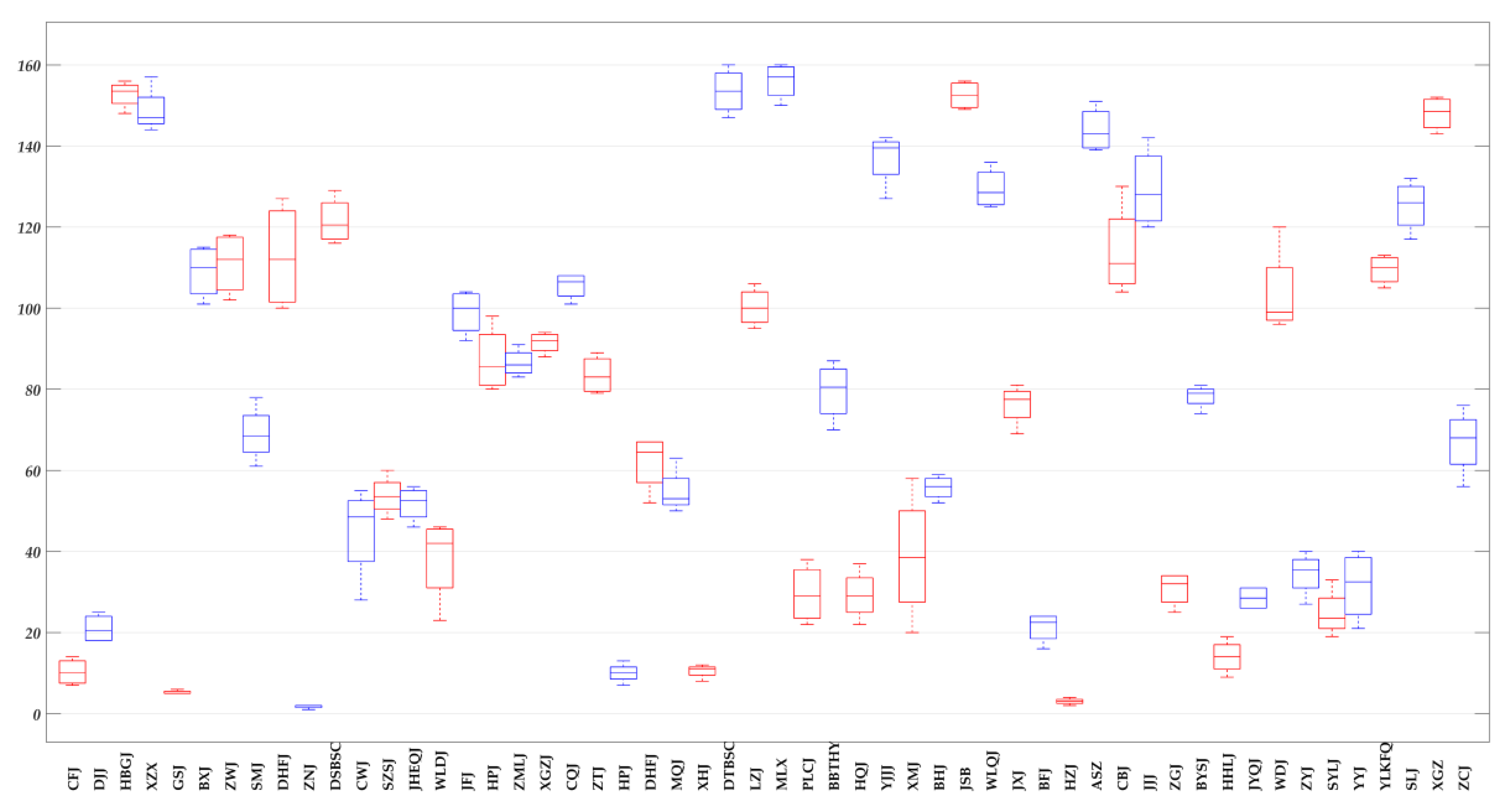
We ranked theft rates (Figure 3) from large to small by quarter as global rankings and used a boxplot (Figure 4) to show the changes in every community’s global ranking over the four time periods (Q1 to Q4, respectively). The boxplot, also known as a box-whisker plot, utilizes five statistics: minimum, first quartile, median, third quartile, and maximum. It can roughly show whether the data are symmetrical, as well as the distribution’s degree of dispersion, and other information, and is useful when comparing several samples.
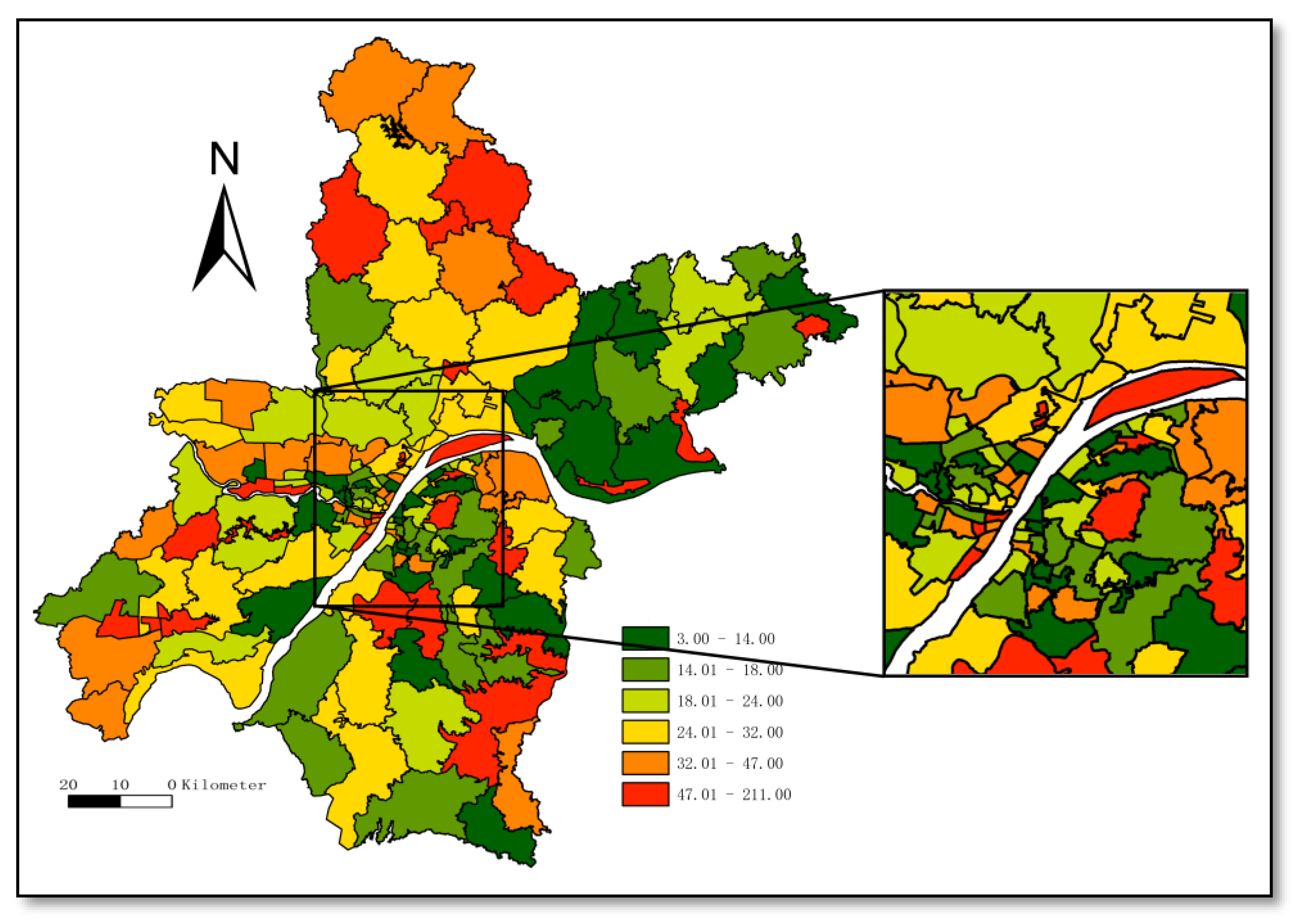
We added the absolute values of the global ranking changes between quarters, showing the changes in each community’s ranking during the four-quarter period. The cumulative change in the global ranking is shown in Figure 5, in which the map is classified by natural breakpoint (Jenks) and the accumulated changes in global rankings in each community over the four time periods ranged from 3 to 211. Figure 5 measures the overall volatility in the rank movements of individual communities.
3.2. Local Crime Exchange Mobility in Wuhan
LIMA can be used to describe the ability of each geographical unit to maintain its own local theft rate rank in the geographical space formed by a certain geographical unit (focal unit) and its geographical neighborhood. The local rank of crime rate (LRCR) concordance between neighboring pairs indicates the spatial distribution of a certain geographical unit (focal unit) defined by its adjacent relation in geographical space. For cross-sectional data, such as that analyzed in this paper, the traditional spatiotemporal method usually models the geographical variables and geographical random effects in a study area in different time slices. Different time slices show different states of spatial heterogeneity, but the relationship between different time slices is not been measured. In other words, the spatial heterogeneity is the result of different times and different effects. In the current study, we were wanted to determine how to metrically measure the spatial differences between different time periods.
If the LIMA value is close to 1, the LRCR of the geographical units in the adjoining geographical space is almost non-exchanging, and any persistent temporal or spatial differences are of interest. If the LIMA value is close to −1, the LRCR of geographical units in the adjoining geographical space and that of the current geographical unit are reversed, meaning any temporal or spatial differences are temporary.
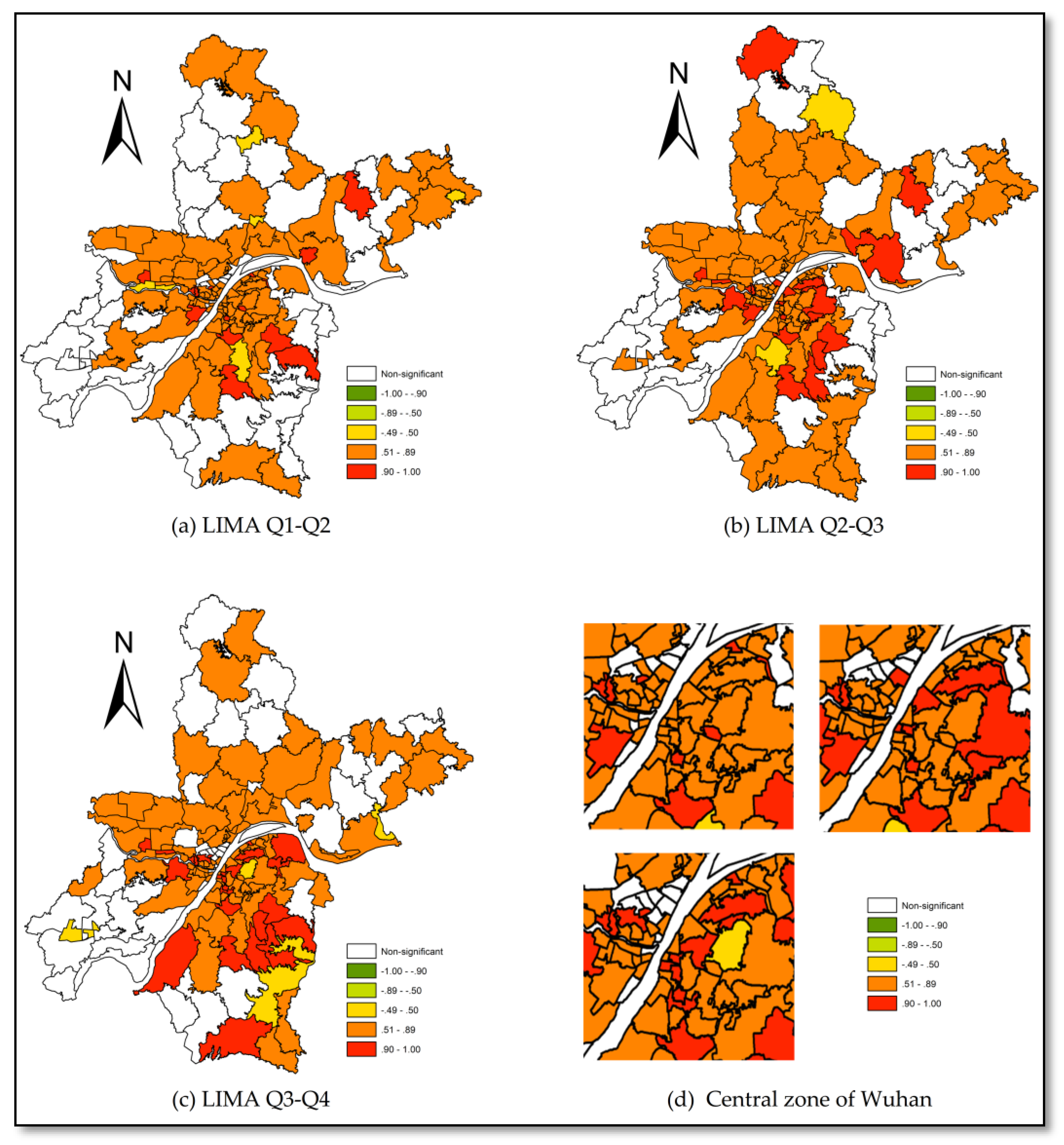
In this way, the LIMA value, ranging from 1 to −1, was used to describe the stability level as high or low, respectively, for the current geographical and adjoining space and allowed us to better understand the temporal and spatial distribution of crime. Of course, the obvious exchange mobility in LRCR is also important, as this value can imply the transfer or temporary suppression of a crime center. In this case, spatial weights were defined using block weights reflecting the geographical units shown in Figure 2. Statistical significance was determined through a Monte Carlo simulation (99 iterations) and significance was defined as p < 0.05 (marked with *), with high significance being defined as p < 0.01 (marked with **). Figure 6 shows the results of this calculation, as determined by Equation (4).
Figure 6 shows that most communities had a positive exchange mobility in the theft rate ranking for each transitional quarter period. Values above 0.9 are marked in red. These values indicate no exchange between pairs of communities, while the ratio for the local rank interchange decreased below 5%, implying that the theft rate rank of most communities barely changed across all 2016 quarters. Values between 0.5 and 0.9 (marked in yellow in Figure 6) indicate that interchanging of local rankings exists in most geographically adjacent communities for a substantial number of community pairs. The local rank interchanges between community pairs in the spatial neighborhood showed ratios from 25% to 5%, although the exchange mobility in space was still mainstream.
For example, the exchange mobility values for Changfu Street, Caidian District, in three quarters were 1.00 **, 0.99 **, and 1.00 **. The adjacent geographical space consists of seven communities, including Daji, Junshan, Tonghu, and Caidian communities, among others. Table 2 shows the global theft rate ranking for each adjoining community from quarter 1 (Q1) to quarter 4 (Q4). Although their global ranks fluctuated slightly, there were no changes in local ranks from the first to the second quarter.
Other geographical units show different temporal and spatial states. For example, Chihui community’s LIMA values over three quarters were −0.25 **, −0.53, and 0.77 **. There are six adjacent geographical spaces to Chihui, including Zoumaling, Changqing, and Yijiadun communities. Table 3 shows the global theft rate ranking for each community, with Chihui Community’s rank declining sharply between the first and second quarters.
3.3. Decomposition of Crime Exchange Mobility in Wuhan
Traditional geographical statistics based on panel data are usually explicit or implicit. They assume all geographical units are homogeneous in the geographical space, while, in fact, each unit belongs to a different district. Although communities may be close geographically, they may be governed by widely divergent administrative means and administrative efficiencies. Therefore, it is unreasonable to compare these subsets using the same metrics. As such, we used the term district to define spatially close relationships between communities in Wuhan. Therefore, we were able to divide the crime exchange mobility into two metrics—one based on the LIMA index within districts and the other based on the dynamic differences between all districts [31].
Table 4 shows the results of applying interregional concordance decomposition to our data. We used regime weights to define neighbor sets as those spatial units belonging to the same region. The diagonal values (marked in gray) indicate the regional exchange mobility measures of the theft rate ranking within all Wuhan districts during the first and second quarters of 2016. The other values measure the exchange mobility among all districts during the corresponding time periods. The values marked with an asterisk indicate significance at p < 0.05 for all 999 Monte Carlo repetitions. The null hypothesis requires that deduction is based on the random spatial displacement of all Wuhan communities’ theft rate rankings. If the ranking of theft rates has a random spatial distribution, the observed exchange mobility of crime rate ranking between or within a district will be significantly different than expected.
The Wuhan districts showed different temporal and spatial evolution patterns in the first and second quarters of 2016. The gray diagonal boxes of Table 4 show that the exchange mobility level of theft ranking was significantly lower than expected using a random spatial pattern. Using Xinzhou District as an example, we see that the exchange mobility level from the first quarter to the second quarter was 0.17, significantly different from the results expected by the null hypothesis (p < 0.01). The result describes the intensity of exchange mobility of community pairs for local theft rate rankings in the different quarters among spatial neighborhoods.
The exchange mobility in Xinzhou District was more intense than that of other districts, and nearly half of its community pairs had interchangeable local ranks. When viewed together with our original data, this confirms that all communities in Xinzhou District have similar theft rate rankings and thus, the differences between them were significantly lower than expected. The average global ranking was 143.25 (out of 160) and there was no obvious crime hot-spot in the district. Similar patterns were found over the next two quarters as well. At the same time, spatial exchange mobility in Xinzhou District increased to 0.45 and 0.48 between the second and third quarters and third and fourth quarters, respectively. While the difference in the theft rate within Xinzhou District rose in comparison to the first quarter, the global ranking of Xinzhou District remained constant at 140.
However, Dongxihu and Huangpi districts showed different exchange mobility patterns. Their overall exchange mobility indexes were around 0.5 larger than that of Xinzhou. Unlike in Xinzhou, there were obvious high-risk areas in Dongxihu and Huangpi. For example, the average global ranking of Dongxihu’s Changqing community was 18, and that of Huangpi’s Qianchuan community was 37.5. The rank correlation (the frequency of rank exchange) was lower for community pairs in Dongxihu and Huangpi districts than in Xinzhou District, which implies the local theft rate ranks in Dongxihu and Huangpi are more stable and that rank exchange only occurs in communities with theft rates similar to that of the local rank. In other words, each district had obvious crime hot and cold spots. For example, over time, the top three most crime-ridden communities in Dongxihu District rotated among Changqing, Jiangjunlu, Huici, Changqinghuayuan, and Jinghe.
The exchange mobilities of the local theft occurrence rank in Wuchang, Jiang’an, and Qiaokou districts were generally higher than in other communities (0.88, 0.89, and 0.90, respectively), and these districts maintained a high exchange mobility measure over time, which means that the local crime rate ranking of each community in the above-mentioned districts remained almost unchanged over time. For example, Qiaokou District showed a high exchange mobility (0.9, p < 0.01). Combining this with observed data, we found that the local ranking only changed for two communities between the first and second quarters: Hanjiadun community (first) and Zongguan community (second). The other communities remained the same, showing a stable spatial distribution of the theft rate ranking in Qiaokou’s main communities (Table 5).
In Table 4, the non-diagonal values measure the shift in the global theft rate ranking between different districts, relative to each another. Values range from −1 to 1. Over time, the global theft rate ranking in two districts gradually weakened. The strength of the global ranking’s ability to facilitate focal unit exchanges between districts describes the stability of the spatial and geographical pattern and the differences in each district’s theft rate ranking.
The districts that showed obvious exchange mobility include Wuchang (1.00 **), Hanyang (1.00 **), Jiang’an (0.96 **), Jianghan (0.93 **), Qiaokou (1.0 **), and Qingshan (0.94 **), all of which are located in downtown Wuhan. The calculation shows that the global theft rate ranking of communities in Xinzhou District changed significantly between the first and second quarters of 2016, which implies a large difference in the theft rates of each community—a difference that changed over time. On the other hand, suburban districts such as Caidian (0.53 **) and Huangpi (0.53 **) showed relatively high levels of exchange mobility, which implies that Xinzhou District has a similar theft rate ranking. Similar space-time situations ewre observed for Huangpi District’s interregional exchange mobility.
Overall, the exchange mobility level of theft in suburban areas was lower (Caidian = 0.69, Jiangxia = 0.65, Huangpi = 0.50 **, Xinzhou = 0.17 **, Dongxihu = 0.54 *, Hannan = 0.33 *) than in the seven downtown areas (Jiang’an = 0.89, Jianghan = 0.81, Qiaokou = 0.90 **, Hanyang = 0.51 *, Wuchang = 0.88, Qingshan = 0.64, Hongshan = 0.67), which implies that communities in suburban areas have smaller differences in global theft rate rankings and that changes in local theft rate rankings are more frequent. In the suburban areas of Wuhan, economy and culture tend to lag behind downtown areas, and these districts have lower amounts of various resources (both aggregate degree and total quantity). This means the differences between communities are relatively smaller than for communities in downtown areas. As such, frequently changing space-time patterns are easily formed, and this affects the local theft rate ranking.
Differences among districts may be caused by natural features, economic development, industrial structure, and policies. Of these, natural features are the most basic and include districts’ differing geographical environments, geologies, landforms, hydrology, animals, plants, and even climate. Economic development also has a large impact on the spatial distribution of crime [26,29]. Finally, different industrial structures influence the performance of specific geographical variables, thus resulting in differences between districts.
4. Conclusions
Continuous urban development has resulted in increasing public security issues, the most common of which are property-related crimes (e.g., theft, burglary, robbery) [29,62,63,64,65,66]. This paper used the concept of exchange mobility with the LIMA method to analyze spatial distribution in relation to the theft rate exchange mobility of theft in Wuhan, China. The goal of traditional spatiotemporal methods or spatial autocorrelation of time variation in crime analysis mainly based on the detection of cross-sectional data characteristics is to show the distribution of criminal events in different geographical units in a study area over multiple time periods. However, the focus of our work was on how to metrically measure the differences in the pattern of crime distribution between different time periods to analyze the dynamics of spatial data based on the crime rate ranking. This is very different to traditional spatiotemporal methods involving time variation in crime. It is important to note that LIMA focuses on different properties of changes in a spatial distribution from those offered by existing spatial autocorrelation or spatial-time static measures. This paper studied the exchange patterns of the spatial distribution of crime events. This could be used as a follow-up research method for space-time modelling and reflects the ability to understand the spatial distribution of criminal incidents in relation to a focal area’s adjacent geographical spaces. Compared to traditional static geographical or space-time methods, it describes the evolution of differing temporal-spatial patterns and differences in the crime rate ranking in one geographical space over different time periods more reasonably. This paper divided the LIMA indexes and, based on the adjacent relationships of Wuhan’s districts, analyzed the intraregional exchange mobility of each district and the interregional exchange mobility between districts. Our results described the stability of the spatial distribution of theft in each district and the changing global ranks between districts. This allowed us to observe the differences in the spatial distribution of criminal incidents in and between districts over time.
LIMA can play a role in actual policing tasks, such as how to optimize the allocation of police resources. Because LIMA describes the degree of stability in the distribution of crime levels (crime rate ranking) in the geographical environment of a geographical unit, it is suitable for the detection of changes in the spatial distribution of crime events. For example, if the value of LIMA in a community is close to 1, it means the crime level of that community is relatively stable; that is, the local crime rate ranking of each community will barely change over time. It is necessary to focus on areas with higher crime levels (higher rank) when distributing the police force according the value of LIMA; that is, the higher the value, the more noteworthy the area in terms of crime. If the LIMA of a community always has a low value, this shows that the local crime level rankings for each community in the geographical space are higher. In other words, the lower the value, the more frequent the changes; thus, the crime environments of the communities are relatively similar because they exchange their local rankings frequently. As such, it is necessary to focus on whether there is a possibility that criminal gangs may commit crimes to cause changes in the crime distribution pattern if there has previously been a community with a high crime ranking in this geographical space. This is information that traditional criminal hot-spot analyses cannot obtain.
To allow the assessment of effectiveness, anticrime initiatives implemented by the police usually cover a limited area, because police resources are always limited. By calculating the LIMA value for a specific geographic unit and comparing it with historical LIMA values, we evaluated whether crime events were less frequent in areas with enhanced police force than those without it, in terms of whether LIMA decreased or if there was a transfer of criminal events.
There are limitations associated with the methods used in this study. First, LIMA must to be interpreted together with observed data and does not have intuitive results, because LIMA studies the exchange patterns of spatial distribution of crime events based on its ranking, causing is a trade-off between potential loss of precision and gain of generality [31]. Thus, the original crime rate data is needed to understand how crime distribution patterns have changed. Second, the scale of the analytical unit needs to be explored further because the choice of spatial/temporal unit influences the results. In this paper, we utilized communities and quarters as analysis units, while further studies have used other spatial scales [67] and high-performance computing to carry out more data intensive calculations [68,69] on much smaller spatial/temporal scales. Third, as the LIMAs are based on ranks, the issues associated with the shift from interval to ordinal measurement scales raise the question of potential loss of sensibility. For example, when the change in the theft rate is not large enough to change the global ranking, it is difficult to identify space-time dynamics through LIMA.
Our future work will focus on the following: (1) how to improve LIMA’s practical value so that it more intuitively describes the exchange mobility between different time periods; (2) how to use LIMA indexes to redistribute and combine areas with similar theft rates and facilitate police to develop management and administrative strategies; (3) how to apply LIMA to smaller spatial scales, such as street segments [67] (this is a major challenge because of the data size of street segments in Wuhan); and (4) conducting more empirical research to examine the specific impacts of crime exchange mobility. Human mobility patterns cause shifts in the baseline population and potentially influence crime statistics [70]. Due to the sensitivity of data, our work did not take the human mobility patterns into account and this will be improved in our future work.
Author Contributions
Conceived and designed the experiments: Y.T., L.D. and L.W. Performed the experiments: Y.T., L.D., X.Z. and W.G. Analyzed the data: Y.T. and W.G. Wrote the paper: Y.T., L.D., X.Z. and L.W.
Acknowledgments
This work has been supported by National key R & D program (2016YFB0502204 and 2017YFB0503704), National Science & Technology Pillar Program [2012BAH35B03], LIESMARS (State Key Laboratory of Information Engineering in Surveying, Mapping and Remote Sensing, Wuhan University) Special Research Funding, and Research on key techniques of dynamic map with position-perceived (Key Open Fund, LIESMARS). The authors are grateful for the valuable comments and suggestions from anonymous reviewers.
Conflicts of Interest
The authors declare no conflict of interest.
References
- Sherman, L.W.; Gartin, P.R.; Buerger, M.E. Hot Spots of Predatory Crime: Routine Activities and the Criminology of Place. Criminology 1989, 27, 27–56. [Google Scholar] [CrossRef]
- Turlach, B.A. Bandwidth Selection in Kernel Density Estimation: A Review. 1998. Available online: https://www.researchgate.net/publication/2316108_Bandwidth_Selection_in_Kernel_Density_Estimation_A_Review (accessed on 1 June 2018).
- Luc, A. Local Indicators of Spatial Association—LISA. Geogr. Anal. 1995, 27, 93–115. [Google Scholar]
- Tobler, W.R. A Computer Movie Simulating Urban Growth in the Detroit Region; Taylor & Francis, Ltd.: New York, NY, USA, 1970; pp. 234–240. [Google Scholar]
- Ord, J.K.; Getis, A. Local Spatial Autocorrelation Statistics: Distributional Issues and an Application. Geogr. Anal. 1995, 27, 286–306. [Google Scholar] [CrossRef]
- Anselin, L.; Getis, A. Spatial statistical analysis and geographic information systems. Ann. Reg. Sci. 1992, 26, 19–33. [Google Scholar] [CrossRef]
- Michael, L. Crime Modeling and Mapping Using Geospatial Technologies; Springer: Dordrecht, The Netherlands, 2013. [Google Scholar]
- Chun, Y.; Griffith, D.A.; Lee, M.; Sinha, P. Eigenvector selection with stepwise regression techniques to construct eigenvector spatial filters. J. Geogr. Syst. 2016, 18, 67–85. [Google Scholar] [CrossRef]
- Getis, A.; Ord, J.K. The Analysis of Spatial Association by Use of Distance Statistics; Springer: Berlin/Heidelberg, Germany, 2010; pp. 127–145. [Google Scholar]
- Chun, Y. Analyzing Space–Time Crime Incidents Using Eigenvector Spatial Filtering: An Application to Vehicle Burglary. Geogr. Anal. 2014, 46, 165–184. [Google Scholar] [CrossRef]
- Murakami, D.; Griffith, D.A. Random effects specifications in eigenvector spatial filtering: A simulation study. J. Geogr. Syst. 2015, 17, 1–21. [Google Scholar] [CrossRef]
- Helbich, M.; Arsanjani, J.J. Spatial eigenvector filtering for spatiotemporal crime mapping and spatial crime analysis. Cartogr. Geogr. Inf. Sci. 2015, 42, 134–148. [Google Scholar] [CrossRef]
- Nakaya, T.; Yano, K. Visualising Crime Clusters in a Space-time Cube: An Exploratory Data-analysis Approach Using Space-time Kernel Density Estimation and Scan Statistics. Trans. GIS 2010, 14, 223–239. [Google Scholar] [CrossRef]
- Roth, R.E.; Ross, K.S.; Finch, B.G.; Luo, W.; Maceachren, A.M. Spatiotemporal crime analysis in U.S. law enforcement agencies: Current practices and unmet needs. Gov. Inf. Q. 2013, 30, 226–240. [Google Scholar] [CrossRef]
- Pereira, M.G.; Caramelo, L.; Orozco, C.V.; Costa, R.; Tonini, M. Space-time clustering analysis performance of an aggregated dataset: The case of wildfires in Portugal. Environ. Model. Softw. 2015, 72, 239–249. [Google Scholar] [CrossRef]
- Uittenbogaard, A.; Ceccato, V. Space-time Clusters of Crime in Stockholm, Sweden. Rev. Eur. Stud. 2012, 4, 1–8. [Google Scholar] [CrossRef]
- Jeong, K.S.; Moon, T.H.; Jeong, J.H. Hotspot Analysis of Urban Crime Using Space-Time. Scan Statistics 2010, 13, 14–28. [Google Scholar]
- Lersch, K.M. Space, Time, and Crime, 3rd ed.; Carolina Academic Press: Durham, NC, USA, 2011. [Google Scholar]
- Adepeju, M.O.; Cheng, T. Determining the Optimal Spatial Scan of Prospective Space-Time Scan Statistics (PSTSS) for Crime Hotspot Prediction; GISRUK: Edinburgh, UK, 2017. [Google Scholar]
- De Melo, S.N.; Pereira, D.V.; Andresen, M.A.; Matias, L.F. Spatial/Temporal Variations of Crime: A Routine Activity Theory Perspective. Int. J. Offender Ther. Comp. Criminol. 2017, 62, 1967–1991. [Google Scholar] [CrossRef] [PubMed]
- Breetzke, G.D.; Cohn, E.G. Seasonal Assault and Neighborhood Deprivation in South Africa Some Preliminary Findings. Environ. Behav. 2012, 44, 641–667. [Google Scholar] [CrossRef]
- Breetzke, G.D. Examining the spatial periodicity of crime in South Africa using Fourier analysis. S. Afr. Geogr. J. 2016, 98, 1–14. [Google Scholar] [CrossRef]
- Schinasi, L.H.; Hamra, G.B. A Time Series Analysis of Associations between Daily Temperature and Crime Events in Philadelphia, Pennsylvania. J. Urban Health 2017, 94, 1–9. [Google Scholar] [CrossRef] [PubMed]
- Rey, S.J.; Montouri, B.D. US Regional Income Convergence: A Spatial Econometric Perspective. Reg. Stud. 1999, 33, 143–156. [Google Scholar] [CrossRef]
- Fields, G.S.; Ok, E.A. The Measurement of Income Mobility: An Introduction to the Literature. Work. Pap. 1996, 71, 557–598. [Google Scholar]
- Aaberge, R.; Björklund, A.; Jäntti, M.; Palme, M.; Pedersen, P.J.; Smith, N.; Wennemo, T. Income Inequality and Income Mobility in the Scandinavian Countries Compared to the United States. Rev. Income Wealth 2002, 48, 443–469. [Google Scholar] [CrossRef] [Green Version]
- Bigman, D.; Srinivasan, P.V. Geographical targeting of poverty alleviation programs: Methodology and applications in rural India. J. Policy Model. 2004, 24, 237–255. [Google Scholar] [CrossRef]
- Webber, D.J.; White, P.; Allen, D.O. Income Convergence across U.S. States: An Analysis Using Measures of Concordance and Discordance. J. Reg. Sci. 2010, 45, 565–589. [Google Scholar] [CrossRef]
- García Velasco, M.M. Regional Policy, Economic Growth and Convergence. Lessons from the Spanish Case. Urban Public Econ. Rev. 2010, 37, 159–162. [Google Scholar] [CrossRef]
- Fields, G.S. Does income mobility equalize longer-term incomes? New measures of an old concept. J. Econ. Inequal. 2010, 8, 409–427. [Google Scholar] [CrossRef]
- Rey, S.J. Space–Time Patterns of Rank Concordance: Local Indicators of Mobility Association with Application to Spatial Income Inequality Dynamics. Mpra Pap. 2016, 106, 1–16. [Google Scholar] [CrossRef] [Green Version]
- Malleson, N.; Andresen, M.A. The impact of using social media data in crime rate calculations: Shifting hot spots and changing spatial patterns. Cartogr. Geogr. Inf. Sci. 2015, 42, 112–121. [Google Scholar] [CrossRef]
- Andresen, M.A.; Malleson, N. Crime seasonality and its variations across space. Appl. Geogr. 2013, 43, 25–35. [Google Scholar] [CrossRef]
- Law, J.; Haining, R. A Bayesian Approach to Modeling Binary Data: The Case of High-Intensity Crime Areas. Geogr. Anal. 2004, 36, 197–216. [Google Scholar] [CrossRef]
- Law, J.; Quick, M.; Chan, P. Bayesian Spatio-Temporal Modeling for Analysing Local Patterns of Crime Over Time at the Small-Area Level. J. Quant. Criminol. 2014, 30, 57–78. [Google Scholar] [CrossRef]
- Wheeler, D.C.; Waller, L.A. Comparing spatially varying coefficient models: A case study examining violent crime rates and their relationships to alcohol outlets and illegal drug arrests. J. Geogr. Syst. 2009, 11, 1–22. [Google Scholar] [CrossRef]
- Gracia, E.; López-Quílez, A.; Marco, M.; Lladosa, S.; Lila, M. Exploring Neighborhood Influences on Small-Area Variations in Intimate Partner Violence Risk: A Bayesian Random-Effects Modeling Approach. Int. J. Environ. Res. Public Health 2014, 11, 866–882. [Google Scholar] [CrossRef] [PubMed] [Green Version]
- Law, J.; Quick, M.; Chan, P.W. Analyzing Hotspots of Crime Using a Bayesian Spatiotemporal Modeling Approach: A Case Study of Violent Crime in the Greater Toronto Area. Geogr. Anal. 2015, 47, 1–19. [Google Scholar] [CrossRef]
- Law, J.; Quick, M. Exploring links between juvenile offenders and social disorganization at a large map scale: A Bayesian spatial modeling approach. J. Geogr. Syst. 2013, 15, 89–113. [Google Scholar] [CrossRef]
- Rey, S.J. Spatial Analysis of Regional Income Inequality. Urban/Regional 2001, 1, 280–299. [Google Scholar]
- Rey, S.J.; Ye, X. Comparative Spatial Dynamics of Regional Systems. In Progress in Spatial Analysis; Springer: Berlin/Heidelberg, Germany, 2010; pp. 441–463. [Google Scholar]
- Rey, S.J.; Gallo, J.L. Spatial Analysis of Economic Convergence; Palgrave Macmillan: Basingstoke, UK, 2009. [Google Scholar]
- Rey, S.J.; Janikas, M.V. STARS: Space-Time Analysis of Regional Systems. Geogr. Anal. 2006, 38, 67–86. [Google Scholar] [CrossRef] [Green Version]
- Rey, S.J.; Janikas, M.V. Regional convergence, inequality, and space. J. Econ. Geogr. 2005, 5, 155–176. [Google Scholar] [CrossRef]
- Huang, L.; Zhu, X.; Ye, X.; Guo, W.; Fang, J. Characterizing street hierarchies through network analysis and large-scale taxi traffic flow: A case study of Wuhan, China. Environ. Plan. B 2016, 43, 276–296. [Google Scholar] [CrossRef]
- Kendall, M.G. Rank correlation methods. Br. J. Psychol. 1955, 25, 86–91. [Google Scholar] [CrossRef]
- Christensen, D. Fast algorithms for the calculation of Kendall’s τ. Comput. Stat. 2005, 20, 51–62. [Google Scholar] [CrossRef]
- Fagin, R.; Ravikumar, S.; Sivakumar, D. Efficient Similarity Search and Classification Via Rank Aggregation. U.S. Patent 10/458,512, 9 December 2004. [Google Scholar]
- Chapelle, O.; Sindhwani, V.; Keerthi, S.S. Optimization Techniques for Semi-Supervised Support Vector Machines. J. Mach. Learn. Res. 2008, 9, 203–233. [Google Scholar]
- Dwork, C.; Kumar, R.; Naor, M.; Sivakumar, D. Rank aggregation methods for the Web. In Proceedings of the 10th International Conference on World Wide Web, Hong Kong, China, 1–5 May 2001; ACM: New York, NY, USA, 2001; pp. 613–622. [Google Scholar] [Green Version]
- Genest, C.; Nešlehová, J.; Ghorbal, N.B. Estimators Based on Kendall’s Tau in Multivariate Copula Models. Aust. N. Z. J. Stat. 2011, 53, 157–177. [Google Scholar] [CrossRef]
- Cherubini, U.; Luciano, E. Value-at-risk Trade-off and Capital Allocation with Copulas. Econ. Notes 2001, 30, 235–256. [Google Scholar] [CrossRef] [Green Version]
- Dardanoni, V.; Lambert, P. Horizontal inequity comparisons. Soc. Choice Welf. 2001, 18, 799–816. [Google Scholar] [CrossRef]
- Dall Aglio, G.; Kotz, S.; Salinetti, G. Advances in Probability Distributions with Given Marginals; Kluwer Academic Publishers: Dordrecht, The Netherlands; Boston, MA, USA; London, UK, 1991; p. 702. [Google Scholar]
- Kepner, W.G.; Watts, C.J.; Edmonds, C.M.; Maingi, J.K.; Marsh, S.E.; Luna, G. A Landscape Approach for Detecting and Evaluating Change in a Semi-Arid Environment; Springer: Dordrecht, The Netherlands, 2000. [Google Scholar]
- Kundzewicz, Z.W.; Robson, A.J. Change detection in hydrological records—A review of the methodology. Hydrol. Sci. J. 2004, 49, 7–19. [Google Scholar] [CrossRef]
- Maceachren, A.M. Map Complexity: Comparison and Measurement. Am. Cartogr. 1982, 9, 31–46. [Google Scholar] [CrossRef]
- Fairbairn, D. Measuring Map Complexity. Cartogr. J. 2006, 43, 224–238. [Google Scholar] [CrossRef]
- Rey, S.J. Fast algorithms for a space-time concordance measure. Comput. Stat. 2014, 29, 799–811. [Google Scholar] [CrossRef]
- Rey, S.J.; Anselin, L. PySAL: A Python Library of Spatial Analytical Methods. Rev. Reg. Stud. 2007, 37, 5–27. [Google Scholar]
- Abdi, H. The Kendall Rank Correlation Coefficient. Cognition 2007, 11, 508–510. [Google Scholar]
- Andresen, M.A. Unemployment, GDP, and Crime: The Importance of Multiple Measurements of the Economy. Can. J. Criminol. Crim. Justice 2015, 57, 35–58. [Google Scholar] [CrossRef]
- Ragnarsdottir, A.G. Investigating the Long-Run and Causal Relationship between GDP and Crime in Sweden. Master’s Thesis, Lund University, Lund, Sweden, May 2014. [Google Scholar]
- Ye, X.; Liu, L. Spatial crime analysis and modeling. Ann. GIS 2012, 18, 157. [Google Scholar] [CrossRef]
- Ye, X.; Wu, L.; Lee, J. Accounting for Spatiotemporal Inhomogeneity of Urban Crime in China. Pap. Appl. Geogr. 2017, 3, 196–205. [Google Scholar] [CrossRef]
- Yue, H.; Zhu, X.; Ye, X.; Guo, W. The Local Colocation Patterns of Crime and Land-Use Features in Wuhan, China. Int. J. Geo-Inf. 2017, 6, 307. [Google Scholar] [CrossRef]
- Melo, S.N.D.; Matias, L.F.; Andresen, M.A. Crime concentrations and similarities in spatial crime patterns in a Brazilian context. Appl. Geogr. 2015, 62, 314–324. [Google Scholar] [CrossRef]
- Ye, X.; Huang, Q.; Li, W. Integrating big social data, computing and modeling for spatial social science. Am. Cartogr. 2017, 43, 377–378. [Google Scholar] [CrossRef]
- Ye, X.; Shi, X. Pursuing Spatiotemporally Integrated Social Science Using Cyberinfrastructure; Springer: New York, NY, USA, 2013; pp. 215–226. [Google Scholar]
- Mburu, L.W.; Helbich, M. Crime Risk Estimation with a Commuter-Harmonized Ambient Population. Ann. Am. Assoc. Geogr. 2016, 106, 804–818. [Google Scholar] [CrossRef]
Figure 1.
Wuhan’s geographical location and community boundaries.

Figure 2.
Wuhan’s districts.

Figure 3.
Distribution of theft rate incidents in Wuhan during the study period.
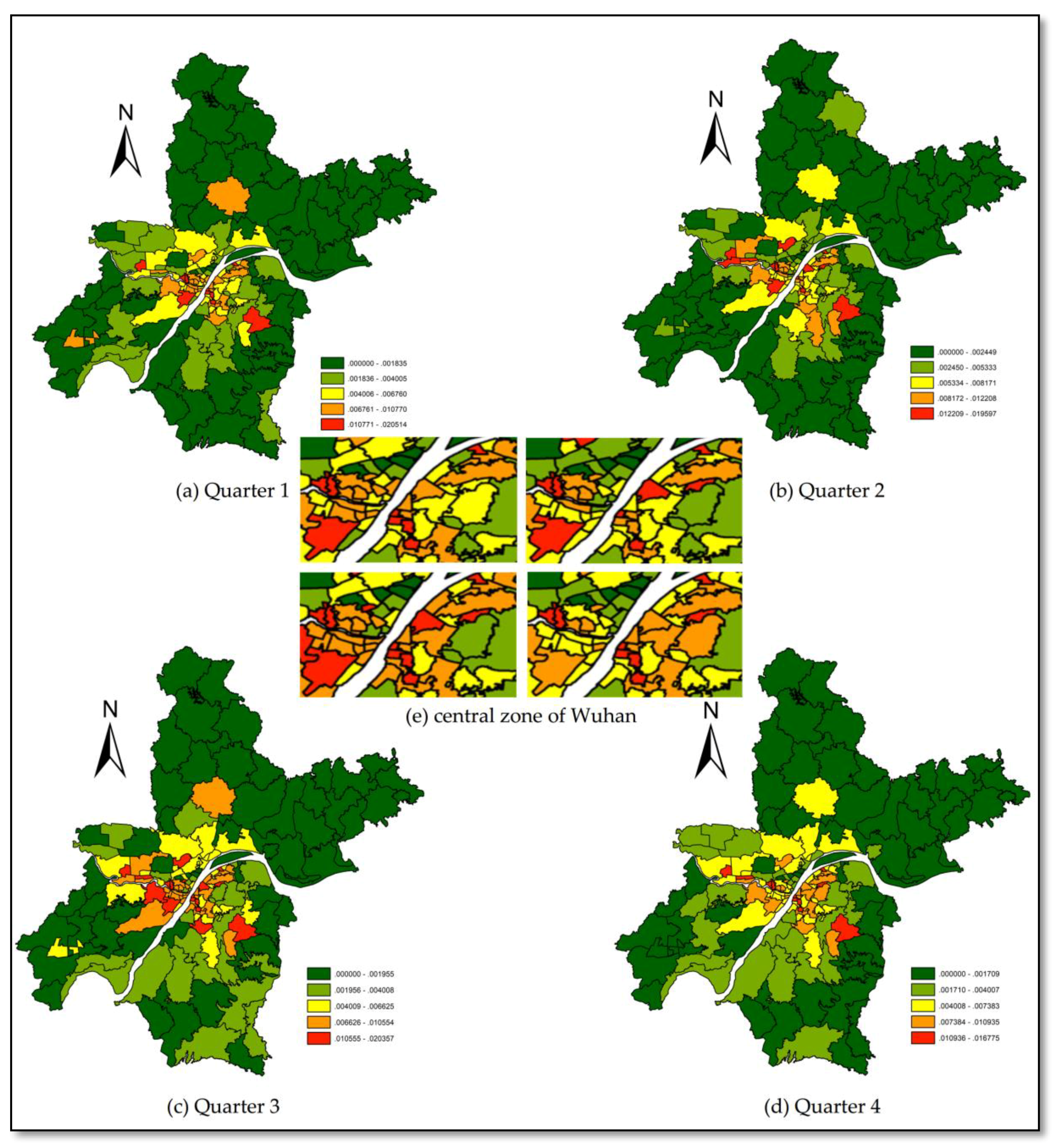
Figure 4.
Changes in global criminal ranking.

Figure 5.
Accumulated mobility of criminal incidents.

Figure 6.
Local Indicator of Mobility Association (LIMA) values in quarters 1–4.


Table 1.
Data summary.
| Name | Format | Time | Primary Property |
|---|---|---|---|
| Case point | Point | 2016 | Case type, time, location, and instruction |
| Spatial unit | Surface | 2010 | Districts and communities |
| Population | Point | 2013 | IDs and addresses |
Table 2.
Global theft rate rank of Caidian Community and adjoining communities.
| Time | Caidian | Daji | Junshan | Tonghu | Jiangti | Zhoutou | Changfu |
|---|---|---|---|---|---|---|---|
| Q1 | 106 | 32 | 4 | 108 | 11 | 73 | 47 |
| Q2 | 109 | 32 | 4 | 100 | 12 | 79 | 44 |
| Q3 | 123 | 22 | 3 | 99 | 10 | 78 | 48 |
| Q4 | 118 | 22 | 4 | 115 | 8 | 85 | 56 |
Table 3.
Global theft rate ranking of Chihui Community and adjoining communities.
| Time | Yijiadun | Jinghe | Zoumaling | Changqing | Wujiashang | Cihui |
|---|---|---|---|---|---|---|
| Q1 | 68 | 53 | 94 | 14 | 22 | 51 |
| Q2 | 110 | 31 | 75 | 10 | 57 | 150 |
| Q3 | 88 | 43 | 84 | 17 | 24 | 28 |
| Q4 | 24 | 51 | 69 | 31 | 21 | 10 |
Table 4.
Breakdown of crime exchange mobility, Q1–Q2.
| Location | DXH | XZ | WC | HN | HY | JX | JA | JH | HS | QK | CD | QS | HP |
|---|---|---|---|---|---|---|---|---|---|---|---|---|---|
| DXH | 0.54 * | 0.76 | 0.69 | 0.48 * | 0.66 | 0.52 ** | 0.59 * | 0.59 * | 0.73 | 0.69 | 0.64 | 0.62 * | 0.56 ** |
| XZ | 0.76 | 0.17 ** | 1.00 ** | 0.92 | 1.00 ** | 0.69 | 0.96 ** | 0.93 * | 0.85 | 1.00 ** | 0.53 ** | 0.94 ** | 0.53 ** |
| WC | 0.69 | 1.00 ** | 0.88 | 0.89 | 0.62 * | 0.85 | 0.91 * | 0.83 | 0.89 * | 0.81 | 0.94 ** | 0.70 | 0.91 ** |
| HN | 0.48 * | 0.92 | 0.89 | 0.33 * | 0.93 | 0.38 ** | 0.70 | 1.00 | 0.88 | 1.00 | 0.76 | 0.70 | 0.68 |
| HY | 0.66 | 1.00 ** | 0.62 * | 0.93 | 0.51 * | 0.89 * | 0.91 * | 0.77 | 0.78 | 0.71 | 0.87 | 0.69 | 0.92 ** |
| JX | 0.52 ** | 0.69 | 0.85 | 0.38 ** | 0.89 * | 0.65 | 0.59 * | 0.71 | 0.83 | 0.76 | 0.71 | 0.77 | 0.56 ** |
| JA | 0.59 * | 0.96 ** | 0.91 * | 0.70 | 0.91 * | 0.59 * | 0.89 | 0.84 | 0.80 | 0.90 | 0.81 | 0.88 | 0.79 |
| JH | 0.59 * | 0.93 * | 0.83 | 1.00 | 0.77 | 0.71 | 0.84 | 0.81 | 0.87 | 0.76 | 0.86 | 0.64 | 0.79 |
| HS | 0.73 | 0.85 | 0.89 * | 0.88 | 0.78 | 0.83 | 0.80 | 0.87 | 0.67 | 0.82 | 0.75 | 0.64 | 0.75 |
| QK | 0.69 | 1.00 ** | 0.81 | 1.00 | 0.71 | 0.76 | 0.90 | 0.76 | 0.82 | 0.90 | 0.90 * | 0.61 | 0.89 * |
| CD | 0.64 | 0.53 ** | 0.94 ** | 0.76 | 0.87 | 0.71 | 0.81 | 0.86 | 0.75 | 0.90 * | 0.69 | 0.77 | 0.57 ** |
| QS | 0.62 * | 0.94 ** | 0.70 | 0.70 | 0.69 | 0.77 | 0.88 | 0.64 | 0.64 | 0.61 | 0.77 | 0.64 | 0.78 |
| HP | 0.56 ** | 0.53 ** | 0.91 ** | 0.68 | 0.92 ** | 0.56 ** | 0.79 | 0.79 | 0.75 | 0.89 * | 0.57 ** | 0.78 | 0.50 ** |
Districts 1–13 are as follows: DXH = Dongxihu, XZ = Xinzhou, WC = Wuchang, HN = Hannan, HY = Hanyang, JX = Jiangxia, JA = Jiangan, JH = Jianghan, HS = Hongshan, QK = Qiaokou, CD = Caidian, QS = Qingshan, and HP = Huangpi. * p < 0.05. ** p < 0.01.
Table 5.
Global theft rate ranking of communities in Qiaokou District.
| Time | Baofeng | Hanjiadun | Hanshuiqiao | Hanzheng | Yijiadun | Changfeng | Zongguan |
|---|---|---|---|---|---|---|---|
| Q1 | 48 | 16 | 40 | 67 | 70 | 95 | 18 |
| Q2 | 37 | 26 | 36 | 62 | 70 | 74 | 14 |
| Q3 | 52 | 13 | 34 | 68 | 69 | 96 | 12 |
| Q4 | 38 | 19 | 29 | 64 | 55 | 90 | 14 |
© 2018 by the authors. Licensee MDPI, Basel, Switzerland. This article is an open access article distributed under the terms and conditions of the Creative Commons Attribution (CC BY) license (http://creativecommons.org/licenses/by/4.0/).
Share and Cite
MDPI and ACS Style
Tang, Y.; Zhu, X.; Guo, W.; Duan, L.; Wu, L. Analyzing Space-Time Dynamics of Theft Rates Using Exchange Mobility. ISPRS Int. J. Geo-Inf. 2018, 7, 210. https://0-doi-org.brum.beds.ac.uk/10.3390/ijgi7060210
AMA Style
Tang Y, Zhu X, Guo W, Duan L, Wu L. Analyzing Space-Time Dynamics of Theft Rates Using Exchange Mobility. ISPRS International Journal of Geo-Information. 2018; 7(6):210. https://0-doi-org.brum.beds.ac.uk/10.3390/ijgi7060210
Chicago/Turabian StyleTang, Yicheng, Xinyan Zhu, Wei Guo, Lian Duan, and Ling Wu. 2018. "Analyzing Space-Time Dynamics of Theft Rates Using Exchange Mobility" ISPRS International Journal of Geo-Information 7, no. 6: 210. https://0-doi-org.brum.beds.ac.uk/10.3390/ijgi7060210
Note that from the first issue of 2016, this journal uses article numbers instead of page numbers. See further details here.