Optical Satellite Image Geo-Positioning with Weak Convergence Geometry

Abstract

High-resolution optical satellites are widely used in environmental monitoring. With the aim to observe the largest possible coverage, the overlapping areas and intersection angles of respective optical satellite images are usually small. However, the conventional bundle adjustment method leads to erroneous results or even failure under conditions of weak geometric convergence. By transforming the traditional stereo adjustment to a planar adjustment and combining it with linear programming (LP) theory, a new method that can solve the bias compensation parameters of all satellite images is proposed in this paper. With the support of freely available open source digital elevation models (DEMs) and sparse ground control points (GCPs), the method can not only ensure the consistent inner precision of all images, but also the absolute geolocation accuracy of the ground points. Tests of the two data sets covering different landscapes validated the effectiveness and feasibility of the method. The results showed that the geo-positioning performance of the method was better in regions of smaller topographic relief or for satellite images with a larger imaging altitude angle. The best accuracy of image geolocation with weak convergence geometry was as high as to 3.693 m in the horizontal direction and 6.510 m in the vertical direction, which is a level of accuracy equal to that of images with good intersection conditions.

1. Introduction

With advantages of wide coverage, short revisit time, and the appropriate spatial resolution required for large-scale mapping, high-resolution optical satellite imagery is an important means of obtaining global geospatial data. In the process of mapping, accurate exterior orientation parameters (EOPs) and the consistent inner precision of the images are essential, which can be obtained using the aerial triangulation method [1]. Aerial triangulation is based on the principle of the intersection of conjugate rays in overlapped images to undertake bundle block adjustment computation. Obviously, the intersection angle is a critical factor that affects geo-positioning accuracy [2]. For stereo mapping satellite, its paths and imaging parameters must be designed specially to ensure the ratio of base-to-height and the intersection angle of stereo image pairs meet the requirement for topography mapping. However, it should be noted that the intersection angle for a stereo model is not always large enough. The availability of pairs with good convergence cannot be assumed at all times, and in particular, heavy reliance on such pairs can impose some limitations on the broad applications of satellite images. The conjugate rays of image pairs with weak convergence geometry are almost parallel, which leads to erroneous results or iteration failures during the bundle block adjustment (BBA). This undesirable situation greatly limits the use of satellite imagery data. Hence, it is necessary to modify the traditional BBA approach to adopt the weakly convergence geometry conditions.

For the geolocation of satellite imagery with good intersection conditions, many studies have been conducted by scholars. As geometry processes with the rational function model (RFM) [3] have no bearing on a specially appointed sensor, RFM has been widely used in the field of remote sensing. Previous studies have revealed that different types of satellite imagery have various levels of geo-positioning accuracy if they rely entirely on the rational polynomial coefficients (RPCs) provided by the vendors. For example, the new breed of DigitalGlobe’s very high resolution satellites (i.e., GeoEye-1 and WorldView-1/2/3/4) have an impressive horizontal geolocation accuracy without ground control points (GCPs) better than 5.0 m (CE90) [4,5,6,7]. Meanwhile, a horizontal error of about 15 m was found for the ZY-3 stereo imagery [8]. Similar investigations have been carried out for various images, such as SPOT [9,10] and Pleiades [11,12].

The above-mentioned studies indicate the continual accuracy improvement and higher potential in optical satellite images for topographic mapping. However, for real mapping applications, the bottleneck has been the availability of recently acquired stereo pairs of good quality. The obtainable geo-positioning accuracy of satellite images is highly relevant to factors such as sensor characteristics and imaging geometry. Orun and Natarajan [13] indicated that a smaller angle of convergence had a significant effect on the elevation accuracy. A weakly convergent angle may cause an elevation error of hundreds of meters or even iteration failures. A quantitative analysis of the intersection angle on the positioning accuracies of stereo pairs was performed by Jeong et al. [14,15], who pointed out that the convergence angle was an important consideration for image geolocation and may significantly affect both the horizontal and vertical accuracies. The effects of convergence angle for stereo pairs were also investigated by Li [16].

Despite the accuracy being low, there have been relatively few studies on the geometric location of the weak intersection image. Aiming to improve the targeting precision of images with weak convergence geometry, Teo [17] advanced a method of utilizing the digital elevation model (DEM) as the elevation control, which could improve the geolocation accuracy, as well as the geometric discrepancies between images. Wang [18] proposed a strategy that used a planar block adjustment method to solve the orientation parameters of all satellite images, and then each satellite image was ortho-rectified. The key technology is the use of the height in the RFM as a known parameter, which can then be interpolated from the DEM. Cheng [19] took the elevation value extracted from the DEM as the observed values with errors, combined the height value, and measured image coordinates to build the adjustment model. In addition, Ping et al. [20] also conducted similar studies. Jaehoon [21] suggested an intersection method to improve the accuracy of a three-dimensional (3D) position with a weak geometry. Zheng [22] proposed a method which was an affine transformation model, and a preconditioned conjugate gradient algorithm was used for producing and updating ortho-maps of large areas. To deal with the weak geometry of the large blocks, a reference DEM was used in this method as an additional constraint in the BBA.

As can be seen from the above studies, one common method to deal with image geolocation with a weak intersection angle is to use the elevation value from the DEM as the known height value in the RFM. In this process, the unknowns of the ground point coordinate recede from 3 to 2, so the ill-condition problem in BBA can be avoided. When the accuracy of the reference DEM is high enough, this method works well. Nonetheless, when the DEM precision is low, errors from the DEM greatly affect the location precision, especially in the vertical direction. Therefore, the planar adjustment method has a technical deficiency and cannot solve the problem completely. Given this circumstance, a modified algorithm which can avoid this shortcoming is presented in this paper. The improved approach can achieve satisfactory results, even with the support of open source DEM.

Linear programming (LP) theory is utilized based on planar block adjustment in this method. The process is divided into two steps. First, a reference DEM, which can be obtained freely, is used for the planar block adjustment method. Second, the result of the planar adjustment is regarded as the initial value of the LP optimization method. Then, the simplex method of LP is applied to solve the unknown parameters. By combining the LP method with plane block adjustment, weak intersection stereo pairs can achieve accuracy equal to that of good convergence image pairs.

LP, as a part of applied mathematics, is seen as a solving method to achieve the best outcome in a mathematical model whose requirements are represented by linear relationships [23]. Based on the existing research, the LP theory was applied to the photogrammetric processing described in this paper to avoid the ill effect from DEM errors and break the technical bottleneck of optical satellite image geo-positioning with weak convergence geometry.

2. Methodology

2.1. Overview of the Proposed Method

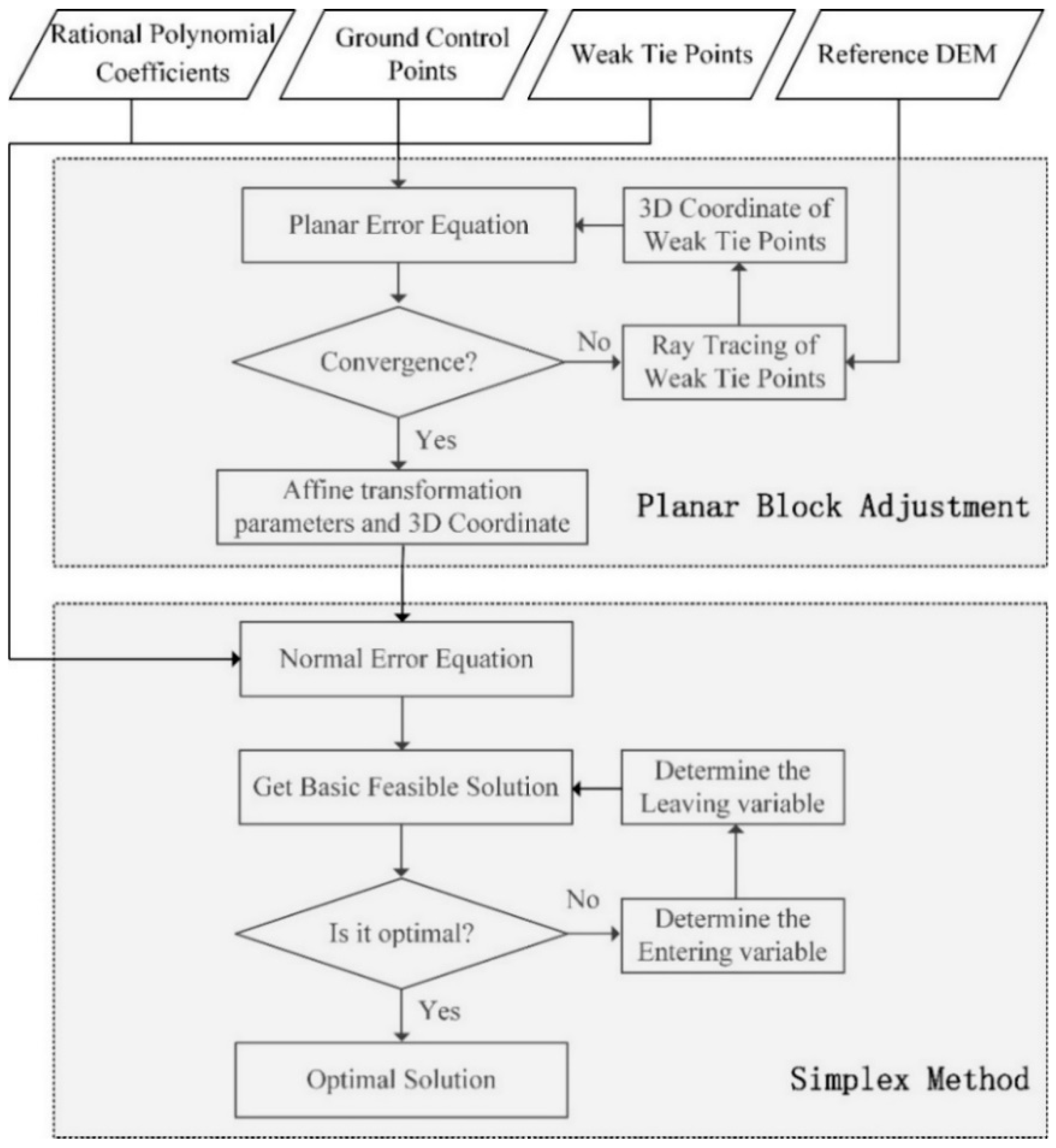
Weak convergence geometry refers to overlapped images with a small intersection angle of imaging lights. At present, there is no clear stipulation on weak intersection image angle tolerance. Generally, intersection angles less than 10° are regarded as a weak convergence geometry condition [17,18,19]. So, strictly speaking, a tie point (TP) that meets the weak convergence condition is defined as a weak tie point (WTP). In fact, we refer to all the TPs on the weak convergence image pairs as WTPs, regardless of the actual intersection angle for convenience. Unless otherwise specified, the TPs mentioned in this article are a general reference and include WTPs. If the conventional method is still used in such situations, the height of the ground point will be abnormal, which leads to adjustment failures to converge. Even if the convergence threshold of the adjustment is reduced, forcing the block adjustment to converge will cause data products to not meet the mapping specifications. To cope with this case, a robust solution for geolocation is proposed in this paper. Two major parts were included in the process. The first was planar block adjustment, while the second part was the simplex method of LP. Using the result of the first step as the good initial value of the second step, and by setting an appropriate constraint value for the unknowns, the orientation parameters of the images and coordinates of ground points can be solved. The workflow of the algorithm is shown in Figure 1.

2.2. The Rational Function Model

With the advantages of simple form and being sensor-independent, the RFM sensor model proposed by Grodecki and Dial [24] was used for the modeling described in this paper. Since the RFM has been fully studied in previous work [24,25,26], only a brief description is provided here.

The RFM uses the ratio of two cubic polynomials to describe the relationship between the image space and the object space. The model equations are expressed as Equation (1).

$$\{\begin{array}{l}{s}_n=\frac{Nu{m}_s\left({\phi }_n,{\lambda }_n,h_n\right)}{De{n}_s\left({\phi }_n,{\lambda }_n,h_n\right)}\\ l_n=\frac{Nu{m}_l\left({\phi }_n,{\lambda }_n,h_n\right)}{De{n}_l\left({\phi }_n,{\lambda }_n,h_n\right)}\end{array}$$

(1)

where $\left(s_n,l_n\right)$ is the normalized image coordinate; $\left({\phi }_n,{\lambda }_n,h_n\right)$ is the normalized ground coordinate.

$Nu{m}_s\left({\phi }_n,{\lambda }_n,h_n\right)$, $De{n}_s\left({\phi }_n,{\lambda }_n,h_n\right)$, $Nu{m}_l\left({\phi }_n,{\lambda }_n,h_n\right)$, and $De{n}_l\left({\phi }_n,{\lambda }_n,h_n\right)$ are the third-order polynomial of the following form:

$$\begin{array}{ll}p=& a_1+a_2{\lambda }_n+a_3{\phi }_n+a_4{h}_n+a_5{\lambda }_n{\phi }_n+a_6{\lambda }_n{h}_n+a_7{\phi }_n{h}_n+a_8{\lambda }_n{}^2+a_9{\phi }_n{}^2+a_{10}{h}_n{}^2+a_{11}{\phi }_n{\lambda }_n{h}_n+\\ & a_{12}{\lambda }_n{}^3+a_{13}{\lambda }_n{\phi }_n{}^2+a_{14}{\lambda }_n{h}_n{}^2+a_{15}{\lambda }_n{}^2{\phi }_n+a_{16}{\phi }_n{}^3+a_{17}{\phi }_n{h}_n{}^2+a_{18}{\lambda }_n{}^2{h}_n+a_{19}{\phi }_n{}^2{h}_n+a_{20}{h}_n{}^3\end{array}$$

where $a_i\left(i=1,2,\cdots ,20\right)$ are the RPCs. The calculation of normalization is as follows:

$$\{\begin{array}{c}{\phi }_n=(\phi -{\phi }_0)/{\phi }_s\\ {\lambda }_n=(\lambda -{\lambda }_0)/{\lambda }_s\\ h_n=(h-h_0)/h_s\end{array}\{\begin{array}{c}{s}_n=(s-s_0)/s_s\\ \\ l_n=(l-l_0)/l_s\end{array}$$

(2)

where $\left(\phi ,\lambda ,h\right)$ are the geodetic longitude, latitude, and height components of the ground coordinate; $\left(s,l\right)$ are the sample and line components of the image coordinate; $s_0,l_0,{\phi }_0,{\lambda }_0,h_0$ and $s_s,l_s,{\phi }_s,{\lambda }_s,h_s$ are the corresponding offset and scale terms.

RPCs and the normalized parameters are stored together in satellite imagery auxiliary files. To maintain numerical precision, the object and image space coordinates are normalized to (−1, +1).

2.3. The Planar Block Adjustment

The planar block adjustment of satellite images refers to a method where only the affine transformation parameters and planimetric coordinates of TPs are solved, while the elevation value is interpolated from the reference DEM in the iteration. In this way, the unknowns of the ground point coordinate recede from 3 to 2, so the negative effect caused by the small intersection angle can be avoided.

Due to the imperfect measurement of satellite ephemeris and attitude, the vendor-provided RPCs are commonly inaccurate. To weaken the impact of the measuring error, the most common solution is to adjust the image coordinates, but not correct the RPCs. Studies have shown that bias compensation of the affine transformation model in the image space can eliminate systematic errors [4,25,26]. The affine transformation model is made up of polynomials of line and sample coordinates, as shown in Equation (3).

$$\{\begin{array}{c}\Delta s=e_0+e_s\cdot s+e_l\cdot l\\ \Delta l=f_0+f_S\cdot s+f_l\cdot l\end{array}$$

(3)

where $\left(\Delta s,\Delta l\right)$ are the differences between the measured and nominal coordinates in an image space; $(e_0,e_s,e_l)$ and $(f_0,f_s,f_l)$ are the bias compensation parameters; and $\left(s,l\right)$ are the coordinates of the image point.

Adding the correction terms $\left(\Delta s,\Delta l\right)$ in the image space by substituting Equation (3) into Equation (1) yields:

$$\{\begin{array}{c}\widehat{s}=s+\Delta s=e_0+e_1\cdot s+e_2\cdot l\\ \widehat{l}=l+\Delta l=f_0+f_1\cdot s+f_2\cdot l\end{array}$$

(4)

where $\left(\widehat{s},\widehat{l}\right)$ are the coordinates of the image point as measured manually, $(s,l)$ are the coordinates of the image point as calculated with the RFM, namely:

$$\{\begin{array}{l}s=s_s\cdot \frac{Nu{m}_s\left({\phi }_n,{\lambda }_n,h_n\right)}{De{n}_s\left({\phi }_n,{\lambda }_n,h_n\right)}+s_0\\ l=l_s\cdot \frac{Nu{m}_l\left({\phi }_n,{\lambda }_n,h_n\right)}{De{n}_l\left({\phi }_n,{\lambda }_n,h_n\right)}+l_0\end{array}$$

(5)

Then, the observation equation can be written as

$$\{\begin{array}{l}{v}_s=e_0+e_1\cdot s+e_2\cdot l-\widehat{s}=e_0+e_1\cdot \left(s_s\cdot \frac{Nu{m}_s\left({\phi }_n,{\lambda }_n,h_n\right)}{De{n}_s\left({\phi }_n,{\lambda }_n,h_n\right)}+s_0\right)+e_2\cdot \left(l_s\cdot \frac{Nu{m}_l\left({\phi }_n,{\lambda }_n,h_n\right)}{De{n}_l\left({\phi }_n,{\lambda }_n,h_n\right)}+l_0\right)-\widehat{s}\\ v_l=f_0+f_1\cdot s+f_2\cdot l-\widehat{l}=f_0+f_1\cdot \left(s_s\cdot \frac{Nu{m}_s\left({\phi }_n,{\lambda }_n,h_n\right)}{De{n}_s\left({\phi }_n,{\lambda }_n,h_n\right)}+s_0\right)+f_2\cdot \left(l_s\cdot \frac{Nu{m}_l\left({\phi }_n,{\lambda }_n,h_n\right)}{De{n}_l\left({\phi }_n,{\lambda }_n,h_n\right)}+l_0\right)-\widehat{l}\end{array}$$

(6)

where $\left(v_s,v_l\right)$ are the residual errors of the image point. By linearizing Equation (6) and expanding it to the first term, the basic error equation of the planar block adjustment can be obtained:

$$\left[\begin{array}{c}{v}_s\\ v_l\end{array}\right]=\left[\begin{array}{cccccccc}\frac{\partial v_s}{\partial e_0}& \frac{\partial v_s}{\partial e_1}& \frac{\partial v_s}{\partial e_2}& \frac{\partial v_s}{\partial f_0}& \frac{\partial v_s}{\partial f_1}& \frac{\partial v_s}{\partial f_2}& \frac{\partial v_s}{\partial \phi }& \frac{\partial v_s}{\partial \lambda }\\ \frac{\partial v_l}{\partial e_0}& \frac{\partial v_l}{\partial e_1}& \frac{\partial v_l}{\partial e_2}& \frac{\partial v_l}{\partial f_0}& \frac{\partial v_l}{\partial f_1}& \frac{\partial v_l}{\partial f_2}& \frac{\partial v_l}{\partial \phi }& \frac{\partial v_l}{\partial \lambda }\end{array}\right]●\left[\begin{array}{c}\Delta e_0\\ \Delta e_{\mathrm{a}}\\ \Delta e_2\\ \Delta f_0\\ \Delta f_1\\ \Delta f_2\\ \Delta \phi \\ \Delta \lambda \end{array}\right]-\left[\begin{array}{c}{\epsilon }_s\\ {\epsilon }_l\end{array}\right]$$

(7)

where $\Delta e_0$, $\Delta e_1$, $\Delta e_2$, $\Delta f_0$, $\Delta f_1$, $\Delta f_2$ are the corrections of the affine transformation parameters; $\left(\Delta \phi ,\Delta \lambda \right)$ are the corrections of the plane coordinates; and ${\epsilon }_s$, ${\epsilon }_l$ are the approximate values of the observation equation.

Equations (7) can be written in matrix form:

$$V=AX-L$$

(8)

where $V$ is the residual vector of the image coordinate observation; $A$ is a partial derivatives vector of unknowns; $L$ is the discrepancy vector; $X$ is the incremental vector of unknowns. It should be noted that $X$ of a TP and a GCP are different. For a TP, $X$ is the incremental vector of affine transformation parameters and plane coordinates; for a GCP, $X$ is the incremental vector of affine transformation parameters.

For stereo adjustment, the initial value of the tie point is commonly determined by forward intersection. However, for images with weak convergence, this method does not work. Supported by a reference DEM and RPCs, the ray-tracing method can address this issue. The specific solution is as follows:

• Use the “height-offset (normalized parameter)” value of the provided RPCs of the image as the first initial elevation value;
• Solve the planimetric coordinates by the DEM and RPCs of a single image;
• Interpolate the new elevation value from the DEM by the planimetric coordinates solved in step 2;
• Repeat steps 1–3 until the elevation difference is less than the set threshold.

For the TP existing in multiple overlapped images, calculate the ground 3D coordinates of each image by the ray-tracing method, and take the average as the initial value of the TP for planar block adjustment.

After the initial value of all unknowns are determined, then the adjustment iteration computation is performed with the support of GCPs, TPs or WTPs, and the DEM. The plane coordinates of the TPs in object space and bias compensation parameters will be refreshed after each iteration. Next, the DEM is adopted as the height constraint. The elevation value $Z$ of the TP is interpolated from the DEM rather than from the intersection of multiple satellite images. Subsequently, the plane coordinates $\left(X,Y\right)$ together with the elevation $Z$ is set as a new ground coordinate value of the TP in the next iteration. Repeat the above procedures until the whole adjustment process has converged. It should be noted that the elevation difference between the two iterations is also one of the considerations when deciding whether to stop the iteration.

2.4. Application of Linear Programming in Geo-Positioning

2.4.1. Mathematical Statement

LP is a technique for the optimization of a linear objective function, subject to linear equality and linear inequality constraints. Its feasible region is a convex polytope, which is a set defined as the intersection of finitely many half spaces, each of which is defined by a linear inequality. Its objective function is a real-valued affine (linear) function defined on this polyhedron. An LP algorithm finds a point in the polyhedron where this function has the smallest value, if such a point exists.

In brief, LP is the process of taking various linear inequalities relating to a situation and finding the best value obtainable under those conditions. Before applying LP to geolocation, the basic principle of LP [27] is first introduced.

Linear programs are problems that can be expressed in canonical form as follows:

Minimize

$$c_1{x}_1+c_2{x}_2+\cdots +c_n{x}_n$$

(9)

Subject to

$$\begin{array}{c}{a}_{11}{x}_1+a_{12}{x}_2+\cdots a_{1n}{x}_n=b_1\\ a_{21}{x}_2+a_{22}{x}_2+\cdots a_{2n}{x}_n=b_2\\ \cdots \cdots \\ a_{m1}{x}_1+a_{m2}{x}_2+\cdots a_{mn}{x}_n=b_m\end{array}\}$$

(10)

and

$$x_i\ge 0\left(i=1,2,\cdots ,n\right),b_i\ge 0\left(i=1,2,\cdots ,m\right)$$

(11)

If a set of vectors $x_1,x_2,\cdots x_n$ only satisfies Equation (10), it is called a feasible solution. If Equations (10) and (11) are satisfied together, it is called the basic feasible solution (BFS). If the BFS satisfies Equation (9), it is called the optimal feasible solution (OFS).

For simplicity, the above formula is expressed in matrix form as follows:

$$\begin{array}{ll}\min & CX\\ \mathrm{s}.\mathrm{t}.& AX=b\\ & X\ge 0，b\ge 0\end{array}\}$$

(12)

where $X$ represents the vector of variables (to be determined); $C$ and $b$ are vectors of (known) coefficients. $A$ is a (known) matrix of coefficients, and the expression to be minimized is called the objective function ($CX$ in this case). $AX=b$ and $X\ge 0，b\ge 0$ are the constraints that specify a convex polytope over which the objective function is to be optimized.

Each solution of feasible solution vectors must be completely non-negative, as required for LP. Obviously, this requirement cannot be satisfied in the solution of image geolocation. To apply the LP method to geolocation, a transformation should be made by replacing variable $x$ with the difference of two non-negative numbers, as shown in Equation (13).

$$\begin{array}{l}{x}_i=x_i^{+}-x_i^{-}\\ x_i^{+}\ge 0,x_i^{-}\ge 0,(i=1,2,\cdots n)\end{array}$$

(13)

The mathematical model of geolocation used for LP calculation are the conventional error equations. The only difference between the planar error equations and the conventional error equations are the object coordinates. The unknowns of the former are plane coordinates $\left(\Delta \phi ,\Delta \lambda \right)$, while the unknowns of the latter are 3D coordinates $\left(\Delta \phi ,\Delta \lambda ,\Delta h\right)$. The error equation used here is:

$$AX-V=L$$

(14)

where $X$ represents the correction vector of the bias compensation parameters ($\Delta e_0$, $\Delta e_1$, $\Delta e_2$, $\Delta f_0$, $\Delta f_1$, $\Delta f_2$) and the correction vector of ground 3D coordinates $\left(\Delta \phi ,\Delta \lambda ,\Delta h\right)$; $A$ is a partial derivatives vector of unknowns; $V$ is the residual vector of the image coordinate observation; and $L$ is the discrepancy vector.

According to Equation (13), the error equation can be rewritten as:

$$A(X^{+}-X^{-})-(V^{+}-V^{-})=L$$

(15)

In the calculation process of LP, $X$ and $V$ are considered as unknowns. Then, the standard form of photogrammetry geolocation by LP can be expressed as:

$$\begin{array}{ll}\min & V^{+}+V^{-}\\ \mathrm{s}.\mathrm{t}.& A(X^{+}-X^{-})-(V^{+}-V^{-})=L\\ & X^{+}\ge 0,X^{-}\ge 0,V^{+}\ge 0,V^{-}\ge 0\end{array}\}$$

(16)

As can be seen from Equation (16), $X^{+}$ and $X^{-}$, $V^{+}$ and $V^{-}$ have the same coefficient. According to linear algebra theory, there can be no non-zero solution between them simultaneously. If $X_i^{+}\ne 0$, $V_i^{-}\ne 0$, then $X_i^{-}=0$, $V_i^{+}=0$, or vice versa. Therefore, the OFS of Equation (16) satisfies the following formula:

$${\displaystyle \sum _{i=1}^n\left|v_i\right|}={\displaystyle \sum _{i=1}^n(v_i^{+}+v_i^{-})}=\min$$

(17)

That is, the OFS is the solution under the condition of “the sum of the absolute residuals is minimized”, which is different from the least-square method. Considering the above situation, the mathematical model of geolocation can be solved according to the LP theory.

2.4.2. Basic Principle of the Simplex Algorithm

The common method of finding the OFS of LP is the simplex algorithm, which has been proven to be quite effective. According to the standard form shown in Equation (12), the simplex algorithm solves LP problems by transferring a BFS to another under the constraints of feasible region with non-increasing values of the objective function until an optimum is reached for certain. The details are as follows.

The matrix $A$, $C$, and $X$ in Equation (12) are divided into the following forms:

$$\begin{array}{l}A=\left[\begin{array}{cc}B& D\end{array}\right]\\ C=\left[\begin{array}{cc}{C}_B& C_D\end{array}\right]\\ X=\left[\begin{array}{cc}{X}_B& X_D\end{array}\right]\end{array}\}$$

(18)

where $B$ is called the basis matrix, which is composed of $m$ linearly independent column vectors in $A$, and the other submatrix is the corresponding result of the partition of the $A$ matrix.

Through Equation (18), the standard form of Equation (12) becomes:

$$\begin{array}{ll}\min & C_B{X}_B+C_D{X}_D\\ \mathrm{s}.\mathrm{t}.& B{X}_B+D{X}_D=b\\ & X_B\ge 0,X_D\ge 0\end{array}\}$$

(19)

There are $n$ unknowns and $m$ equations in the constraint in Equation (19), and $n>m$. The solutions of $n$ unknowns can be obtained by $m$ equations, and the rest of $(n-m)$ unknowns can be regarded as 0. If the solution is non-negative, it is the BFS. However, what we are looking for is the OFS.

Supposing the initial feasible solution corresponding to the basis matrix is:

$$X=\left[\begin{array}{cc}{X}_B& 0\end{array}\right]X_D=0$$

(20)

Substituting Equation (20) into the second equation in Equation (19), $X_B$ can be obtained:

$$X_B=B^{-1}b$$

(21)

Equation (21) corresponds to the result of $X_D=0$. If there are any non-zero $X_D$ values, the corresponding $X_B$ value can be obtained by the second formula in Equation (19):

$$X_B=B^{-1}b-B^{-1}D{X}_D$$

(22)

The BFS obtained in Equation (21) is more optimized than the initial feasible solution of Equation (20), which is decided by the discriminant number $r$. Under consideration of Equation (22), let the objective function in Equation (19) be equal to $z$, then:

$$\begin{array}{ll}z& =C_B{X}_B+C_D{X}_D\\ & =C_B\left(B^{-1}b-B^{-1}D{X}_D\right)+C_D{X}_D\\ & =C_B{B}^{-1}b+\left(C_D-C_B{B}^{-1}b\right)C_D\end{array}$$

(23)

As can be seen from the above equation, the first term on the right side of the equation is the objective function value obtained from the previous BFS. Whether it is advantageous to replace a certain component of $X_{{\rm B}}$ with a certain component of $X_D$ depends on the discriminant number $r$:

$$r=C_D-C_B{B}^{-1}b$$

(24)

As $X_D\ge 0$, so long as the discriminant number $r<0$, there must be a better solution than the previous one. If $r\ge 0$, it indicates that the OFS has been obtained. This is the basic idea of the simplex method to find the OFS.

In the process of image geo-positioning with weak convergence geometry, the approximate formula of constraint conditions is listed after the linearization of the condition equation, then the OFS is obtained by the method of gradually approaching. It should be noted in the iteration that the coefficients of $V$ in the error equations are both 1, while the constant terms are not always greater than 0, which is a characteristic of photogrammetry processing. To meet the demands of the simplex algorithm, a component of $b$ that is less than 0 should be multiplied by −1. This situation deserves special attention, and the sign in each iteration must be changed, otherwise the correct answer cannot be obtained.

The theoretical basis of the LP method improving the accuracy of the geo-positioning with weak intersection angle is finding the OFS from the set of BFSs obtained from the constraint conditions to achieve the goal of optimization—minimizing the sum of the absolute residuals. However, this method has the disadvantage of being sensitive to the initial value and searching step length. In this work, the shortcoming was overcome by combining the planar block adjustment with the LP theory. The result of the planar block adjustment was used as the good initial value of the simplex method and a suitable constraint range was set for the unknown parameters. Then, the bias compensation parameters and the ground 3D coordinates of the TPs were solved by the gradually approaching strategy.

3. Experiment

3.1. Test Data

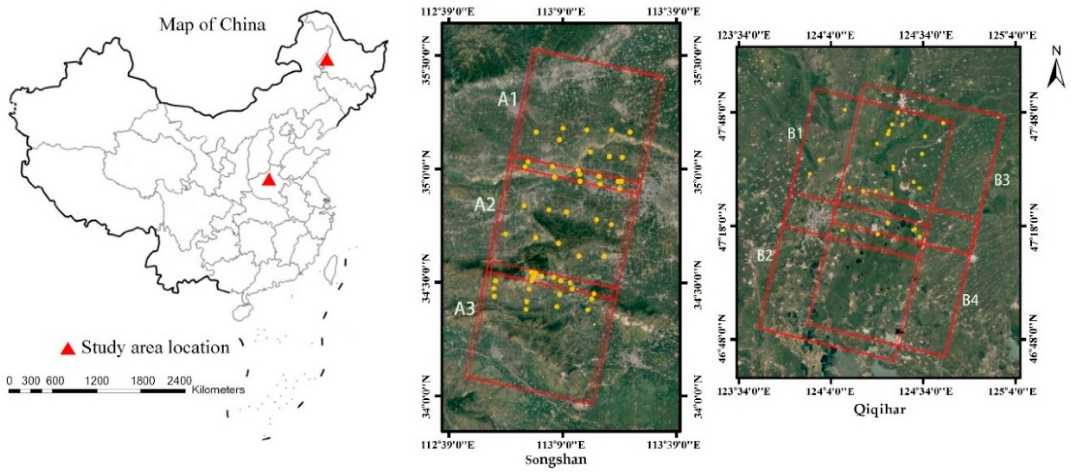
Two different geomorphological data sets were chosen as the study area: the Songshan district and the Qiqihar district in China. The Songshan area consisted of single-track data obtained by ZY-3 in May 2017. The ZY-3 satellite is a stereo mapping satellite, which consists of a three-line camera (TLC) that points forward, backward, and at the nadir. There were three scenes (A1, A2, and A3) in the Songshan area with a total of nine images. The area is located in Henan Province in central China, where mountains constitute the dominant terrain. The maximum height relief is about 1500 m. Fifty-two GCPs were distributed evenly throughout the data set. Meanwhile, the Qiqihar study area included two-track data obtained by TH-1 in September 2015 and March 2016. TH-1 has a similar TLC to the ZY-3 satellite. Four scenes (B1, B2, B3, and B4) were included in the Qiqihar study area for a total of 12 images. This area is in the northeast of China where the maximum terrain relief is about 80 m and belongs to the plain landform. There were 26 GCPs distributed in the Qiqihar area. The ground coverage area and the distribution of GCPs are shown in Figure 2. All images of the two data sets are attached with RPC files. The difference is that the data in the Songshan area were of the 1A level, the RPCs of which are generated by the original ephemeris data in orbit; the Qiqihar area data were at a 1B level, where the RPCs are generated after the ground refinement processing.

The GCPs used in the two data sets were outstanding points, properly selected to determine the locations of the objects, such as road intersections. These points can be accurately identified in both photos and on the ground. The object coordinates of GCPs in the two data sets were obtained in different ways. For the Songshan area, the object coordinates of GCPs were obtained from a high-precision survey product, which had an accuracy at the decimeter level. Meanwhile, the GCPs used in the Qiqihar area were obtained by differential GPS (Global Positioning System) measurement with an average accuracy better than 5 cm. The corresponding image coordinates of the two sets of GCPs were both measured manually. In addition, to ensure the consistent inner precision of images, 25 and 32 TPs were extracted from the images in the Songshan area and Qiqihar area, respectively.

ZY-3 and TH-1 are both stereo mapping satellites that utilize an onboard TLC, which consists of three independent cameras looking forward, at the nadir, and backward, respectively. The forward and backward cameras are tilted at a certain angle with respect to the nadir camera, thereby forming a good intersection condition. During the flight of the satellites, the angle of each camera is almost invariable, resulting in the imaging light of the adjacent two scenes acquired by the same camera to be almost parallel. The image pairs are in a state of weak convergence geometry.

We selected images of two different landforms acquired by the different stereo mapping satellites as the study data. On the one hand, the validity of the algorithm proposed in this paper could be fully verified; on the other hand, it could be compared with the positioning results of images with a good intersection angle. Therefore, objective and fair conclusions could be drawn.

3.2. Experimental Scheme Design

To fully verify the effectiveness of the proposed algorithm, the intersection angles of the overlapped images in the two data sets were first calculated. Based on this, several sets of experiments with different purposes were designed, including the contrast experiment of the planar and stereo block adjustment, the accuracy of the planar block adjustment with open source DEMs, and a geometric positioning experiment of images with weak convergence geometry. The same set of GCPs and independent check points (ICPs) was utilized for each test area to ensure objectiveness. The main comparison tests are described below. The processing of all forward, nadir, and backward images in planar adjustment are abbreviated as F, N, and B in each scheme. The accuracy statistics of the ICPs were based on the Universal Transverse Mercator (UTM) coordinate.

3.2.1. Test 1: Comparison between Planar and Stereo Block Adjustments

This test was conducted to verify the accuracy that could be achieved by the planar block adjustment and make a contrast with the stereo block adjustment with or without GCPs.

• Scheme 1

Free network stereo adjustment using all images without GCPs, with all GCPs set as ICPs.

• Scheme 2

Free network planar adjustment using all forward, nadir, and backward images without GCPs, respectively, with all GCPs set as ICPs. The DEM with a grid size of 10 m × 10 m was set as the height constraint.

• Scheme 3

Controlled network stereo adjustment using all images with enough GCPs, with the rest of the GCPs set as ICPs.

• Scheme 4

Controlled network planar adjustment using all forward, nadir, and backward images with enough GCPs, respectively, with the rest of the GCPs set as ICPs. The DEM with a grid size of 10 m × 10 m was set as the height constraint.

3.2.2. Test 2: Verify the Effect of Open Source DEMs on Planar Adjustment

In this test, open source DEMs—Shuttle Radar Topography Mission (SRTM) and Advanced Spaceborne Thermal Emission and Reflection Radiometer (ASTER) DEMs—that could be obtained freely were set as the height control. The data used for planar adjustment were all still forward-, nadir-, or backward-looking images which were in a state of weak convergence. The configuration of GCPs remained as per Test 1. The purpose of this test was to verify the effectiveness of the algorithm with publicly available DEM data products on the one hand and verify the influence of the DEM accuracy on the planar adjustment on the other hand.

• Scheme 1

The SRTM DEM data with a grid size of 90 m × 90 m are used for elevation control. Free network planar adjustment is executed.

• Scheme 2

The SRTM DEM data with a grid size of 90 m × 90 m are used for elevation control. Controlled network planar adjustment is executed.

• Scheme 3

The ASTER DEM data with a grid of 30 m × 30 m are used for elevation control. Free network planar adjustment is executed.

• Scheme 4

The ASTER DEM data with a grid of 30 m × 30 m are used for elevation control. Controlled network planar adjustment is executed.

3.2.3. Test 3: Geolocation Experiments of Weak Intersection Images

This test was conducted to verify the influence of the number and distribution of GCPs on the proposed algorithm. In addition, to validate whether the conventional method is applicable under the conditions of weak geometric convergence, the BBA was also carried out. The initial values of the simplex method and BBA were both provided by the planar adjustment. Schemes 1–3 were performed by the simplex method; Schemes 4–6 were performed by the BBA. Furthermore, the data used were all forward, nadir, and backward images.

• Scheme 1

Perform the simplex method with two GCPs, which are laid out at the center of the overlapped area along the track.

• Scheme 2

Perform the simplex method with four GCPs, which are laid out at each of the four corners of the overlapped area along the track.

• Scheme 3

Based on Scheme 2, another four GCPs are added and evenly distributed in the coverage.

• Scheme 4

Perform the BBA with two GCPs, which are laid out at the center of the overlapped area along the track.

• Scheme 5

Perform the BBA with four GCPs, which are laid out at each of the four corners of the overlapped area along the track.

• Scheme 6

Based on Scheme 5, another four GCPs are added and evenly distributed in the coverage.

4. Results and Discussion

4.1. Calculation of Intersection Angle of Overlapped Images

For mapping satellites, the TLC has a fixed design angle, resulting in very small intersection angle of overlapped images acquired by the same sensor. However, how small the angle is remains unknown. Therefore, it was necessary to calculate the intersection angle to quantitatively analyze the algorithm described in this paper.

The calculation of intersection angle is based on the method of the line-of-sight vector. First, we extracted a certain number of evenly distributed homologous points in the overlapped area. Second, we calculated the space vectors of the conjugate ray according to the RPCs and two different elevation values. Then, we solved the angle between the two space vectors to obtain the intersection angle of the conjugate ray. Finally, we took the average of the angles of all homologous rays as the intersection angle of the corresponding overlapped images. It should be noted that the geodetic coordinates need to be converted into Universal Transverse Mercator (UTM) coordinates when solving the intersection angles.

According to the above method, the intersection angles of all overlapped images were obtained. Partial typical data (A1 and A2, B1 and B3) were selected as shown in

Table 1. The intersection angles of overlapped images.

Images	Intersection Angle (°)			Images	Intersection Angle (°)
	A1-F 1	A1-N	A1-B		B1-F	B1-N	B1-B
A2-F	0.006	23.842	47.693	B3-F	2.323	27.890	55.285
A2-N	23.840	0.005	23.851	B3-N	27.190	2.734	27.914
A2-B	47.683	23.843	0.006	B3-B	54.579	27.243	2.588

¹ F represents the forward image, likewise, N and B are the abbreviation for nadir and backward images.

.

A1 and A2 were the same orbital data, while B1 and B3 were different orbital images obtained at different times, both of which were very representative. As can be seen from Table 1, the intersection angle of the TLC images formed by ZY-3 and TH-1 were both good and met the design criteria.

Due to its short imaging interval time, the attitude of the sensor was basically unchanged, and the intersection angle of the same orbital images was approximately 0°. In contrast, the imaging interval of different tracks was relatively long. In this process, the attitude of sensors had a certain change, resulting in a slightly larger intersection angle than the data of the same track. However, it was still in a weak convergence state. In a word, regardless of whether the same orbit or different orbit images were obtained by the same sensor, the intersection angles were too small to meet the requirements of stereo-compilation. Reliable results cannot be obtained by the conventional method.

4.2. Test 1: Comparison between Planar and Stereo Block Adjustments

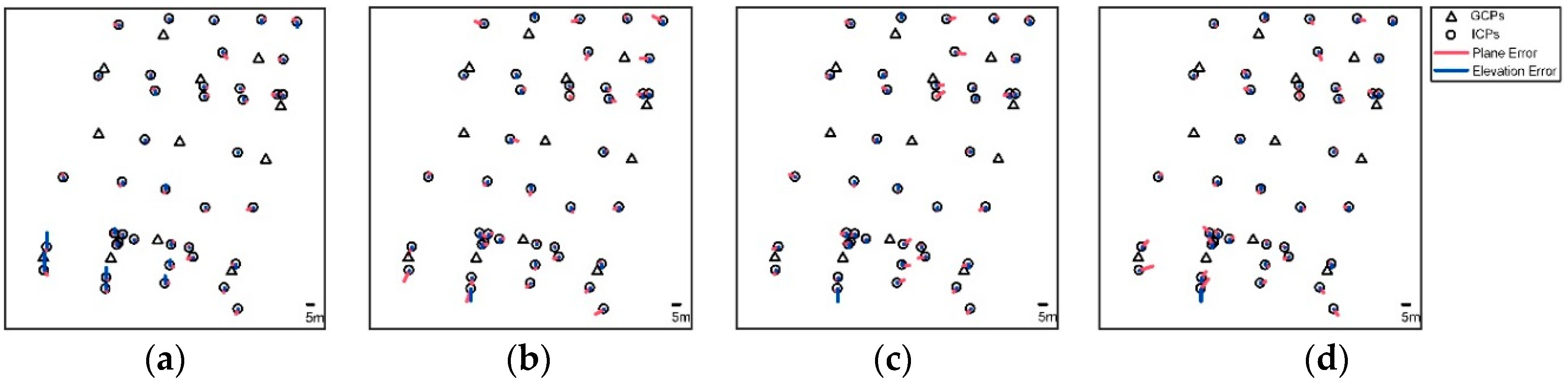
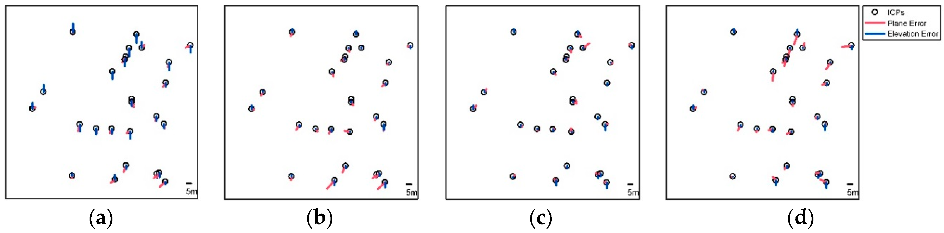
According to the experimental scheme described in Section 3.2, the statistics on the accuracy of the ICP results of Test 1 are listed in

Table 2. Results of planar and stereo block adjustments.

Test Area	Scheme	GCPs	ICPs	Maximum Residual (m)				RMS Error (m)
				X	Y	Plane	Elevation	X	Y	Plane	Elevation
Songshan	1	0	52	43.586	54.186	65.639	21.677	37.226	49.669	62.070	13.389
	2-F	0	52	39.477	57.676	68.755	13.820	27.612	49.444	56.632	3.952
	2-N	0	52	47.893	55.614	72.168	12.916	40.157	45.290	60.529	3.881
	2-B	0	52	51.175	62.743	79.258	12.942	43.866	54.009	69.579	4.216
	3	12	40	3.585	6.002	6.110	7.645	2.082	2.490	3.246	2.551
	4-F	12	40	10.544	8.406	10.725	11.316	3.650	3.231	4.875	2.603
	4-N	12	40	8.370	4.463	9.039	11.306	3.761	2.237	4.376	2.580
	4-B	12	40	5.647	7.576	7.666	12.272	2.226	3.083	3.802	2.622
Qiqihar	1	0	26	6.929	8.126	9.131	10.549	3.013	5.235	6.040	6.958
	2-F	0	26	9.142	9.936	13.502	6.729	3.831	4.876	6.201	2.965
	2-N	0	26	7.188	5.724	9.189	6.872	2.810	2.624	3.845	3.057
	2-B	0	26	11.643	11.882	12.580	6.872	4.120	5.439	6.824	3.248
	3	10	16	5.265	4.584	6.358	4.591	2.789	2.087	3.484	1.844
	4-F	10	16	6.340	6.133	7.651	6.780	3.460	3.197	4.711	2.962
	4-N	10	16	4.799	8.196	9.196	6.872	2.268	2.868	3.656	2.942
	4-B	10	16	8.516	6.359	10.628	6.872	3.133	3.256	4.519	3.087

. In addition, the residual distribution of ICPs of each scheme are drawn, as shown in Figure 3, Figure 4, Figure 5 and Figure 6.

The test results showed that planar adjustment was feasible if the accuracy of the reference DEM data was sufficiently high. With an even distribution of GCPs, the two data sets could achieve a plane accuracy of 3.802 m and 3.656 m by planar adjustment. This indicated that in the planar block adjustment with weak convergence geometry, the reference DEM had the same effect as the height constraint produced by a good intersection condition. In addition, by ignoring the elevation results, the plane accuracy of planar adjustment with fewer images could still reach the same level as the plane accuracy of stereo block adjustment, whether it be a free network or controlled network.

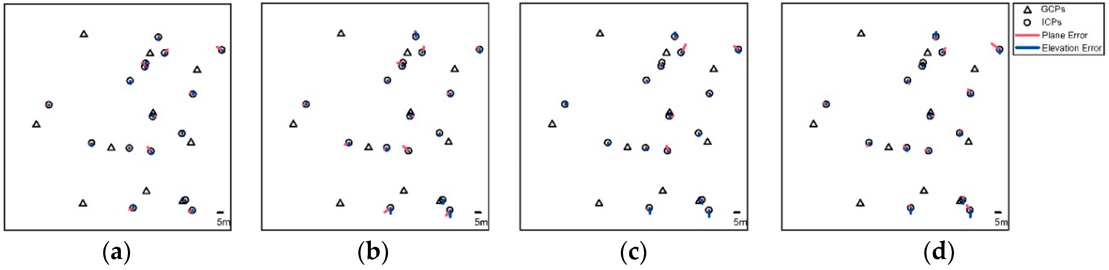
It can be seen from Figure 3 and Figure 5 that the lengths and directions of the residuals of the free network were relatively consistent in each plot. The direction consistence indicated that the positioning results of the two test areas both had systematic errors, while the length was indicative of the level of systematic error. Apparently, the systematic error of the Songshan test area was larger and more obvious. The RPCs of the Songshan area were generated by the direct-transmission attitude and orbit parameters with measurement errors, while the RPCs of the Qiqihar were refined by geometric calibration. Though there was a big difference of the free network adjustment, the accuracy of the controlled network adjustment was at the same level and the systematic errors were effectively eliminated, as shown in Figure 4 and Figure 6. The reason for this is that after a certain number of GCPs were incorporated into the adjustment, the control space basis was determined by the GCPs. Then, the systematic errors were compensated, and the random errors were assigned reasonable values by the least-squares method.

4.3. Test 2: Verify the Effect of Open Source DEMs on Planar Adjustment

Given the good results of Test 1, the precision of the reference DEM was relatively high, which was not always available. In this test, freely available open source DEMs (SRTM and ASTER) were used to make a detailed analysis of the planar adjustment. The edition of SRTM used in the test was SRTM3 DEM V4.1 with a grid size of 30 m and nominal absolute vertical and planimetric accuracies of 16 m (LE90) and 20 m (CE90) [28]. ASTER DEM V2 was used, which is an improved version of V1, with a grid size of 30 m and an absolute vertical accuracy of 17.01 m (LE95) [29]. Previous study has shown that a certain degree of systematic errors existed in the SRTM DEM and ASTER DEM in a local small area [30]. Before the planar adjustment was applied, the actual accuracy of the two DEMs in Songshan and Qiqihar were evaluated by ICPs. The statistical results are shown in

Table 3. The accuracy of Shuttle Radar Topography Mission (SRTM) DEM and Advanced Spaceborne Thermal Emission and Reflection Radiometer (ASTER) DEM.

Area	RMS Error (m)
	SRTM DEM	ASTER DEM
Songshan	22.065	17.036
Qiqihar	9.136	18.476

.

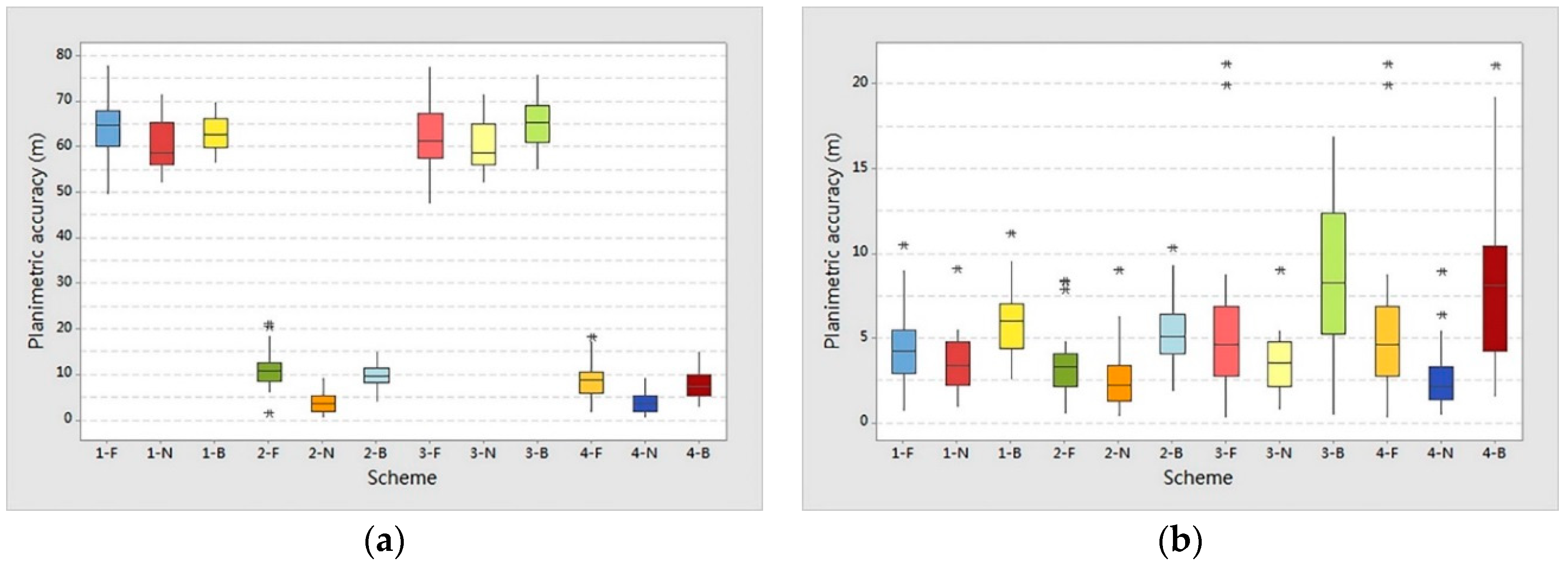
The results of planar adjustment with SRTM DEM and ASTER DEM are shown in Figure 7.

Figure 7 shows the box plots of ICPs. Each box represents the result of a scheme, the edges correspond to the 25th and 75th percentiles, the black central line in the box indicates the median, and the asterisk represents the extreme data points. From Figure 7, we can see that, even with the use of open source DEMs, the consistent planimetric accuracy of the planar adjustment with weak convergence geometry could still be achieved. Despite the different precision, the SRTM and ASTER DEM imposed the same height constraint on the geolocation. With a certain number of GCPs, the planimetric accuracy of forward and backward images was better than 10 m, while the nadir images could be up to 5 m.

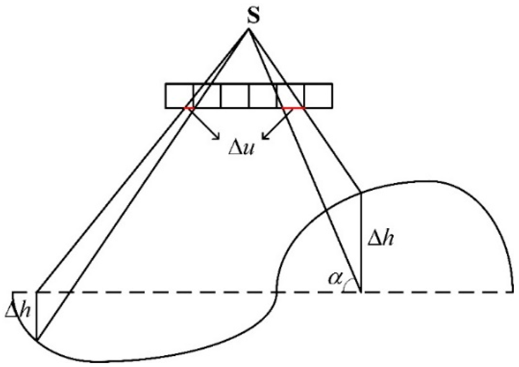
It can also be seen from the statistical results that the plane accuracy of Qiqihar was better than that of Songshan, and the plane accuracy of the nadir image was better than that of the forward and backward images in the same data. The reason for this was the projection difference caused by the topographic relief. The effect of topographic relief is shown in Figure 8.

From Figure 8, we can see that the projection difference is related to the elevation difference and the imaging altitude angle. The imaging altitude angle refers to the angle between the imaging light and the ground. The larger the height difference of the ground, the larger the projection difference; the smaller the imaging altitude angle, the larger the projection difference. The Songshan area consists of hilly terrain, so its topographic variation is larger than Qiqihar, so the positioning accuracy is worse. The nadir image was similar to the vertical observation image, which meant that the camera was perpendicular to the ground, so the projection difference caused in the image by a region of topographic relief was smaller than the forward and the backward images. Therefore, this means that if only the planar adjustment is performed, a higher precision DEM is recommended in the case of high topographic relief or satellite images with large side-sway angles. Moreover, it should be noted that the GCPs and TPs could not be close to the artificial buildings. The reason is that DEM does not contain elevation information of artificial buildings, so GCPs or TPs that lay on artificial buildings will cause statistical error to increase.

4.4. Test 3: Geolocation Experiments of Weak Intersection Images

Based on the results of Test 2, further processing of the simplex method and BBA was performed. With the support of same initial values and same configuration of GCPs, the conventional BBA was still not functioning properly. Schemes 4–6 all failed. The BBA either produced ridiculously wrong results or did not converge at all. The failure of BBA is due to the serious ill condition of normal equation, which is caused by the small intersection angle. For lack of additional constraints, the condition number of normal equation is very large, a small disturbance can trigger a dramatic change in the solution of the equation. In theory, the BBA is based on L2–norm method, also known as least-squares estimation, which is used to minimize the residual sum of squares. On the other hand, the simplex method is based on L1–norm method, also known as least absolute deviation estimation, which is used to minimize the sum of absolute residuals. The weaknesses of the least-squares method are the effect of gross measurement error on the solution and the disturbance and absorbance of error on the solution. However, L1–norm is affected very little by gross error, if at all [31]. The failure indicates that the conventional method is unable to handle image geo-positioning under such extreme imaging geometry. Because of the better robustness and the additional constraints of unknowns, the simplex method shows satisfactory performance. The results of Schemes 1–3 are shown in

Table 4. Results of images geolocation with weak convergence geometry.

Test Area	DEM	Scheme	GCPs	ICPs	RMS Error (m)
					X	Y	Plane	Elevation
Songshan	SRTM	1-F	2	50	15.750	24.822	29.397	18.542
		1-N	2	50	15.116	15.838	21.894	17.460
		1-B	2	50	20.728	18.615	27.860	17.697
		2-F	4	48	3.024	10.344	10.777	14.984
		2-N	4	48	3.629	2.496	4.405	14.338
		2-B	4	48	3.230	9.759	10.279	15.051
		3-F	8	44	3.536	6.696	7.572	12.737
		3-N	8	44	3.217	3.033	4.421	12.089
		3-B	8	44	3.256	7.541	8.214	12.179
	ASTER	1-F	2	50	15.863	24.018	28.784	16.862
		1-N	2	50	15.437	14.111	20.914	16.595
		1-B	2	50	16.281	19.895	25.707	17.848
		2-F	4	48	2.838	8.361	8.829	12.376
		2-N	4	48	3.607	2.493	4.384	11.294
		2-B	4	48	3.164	7.814	8.430	11.767
		3-F	8	44	4.053	6.739	7.864	9.268
		3-N	8	44	2.676	3.503	4.408	9.401
		3-B	8	44	3.683	6.886	7.809	9.751
Qiqihar	SRTM	1-F	2	24	3.054	5.379	6.185	7.255
		1-N	2	24	3.140	4.129	5.188	7.213
		1-B	2	24	2.580	6.334	6.839	7.710
		2-F	4	22	2.513	3.893	4.633	6.797
		2-N	4	22	2.829	2.928	4.071	6.751
		2-B	4	22	2.983	3.960	4.957	6.268
		3-F	8	18	3.379	2.041	3.948	6.401
		3-N	8	18	2.663	2.558	3.693	6.510
		3-B	8	18	2.240	3.145	3.861	6.578
	ASTER	1-F	2	24	3.204	7.914	8.538	12.175
		1-N	2	24	2.958	6.544	7.181	12.511
		1-B	2	24	3.225	9.122	9.675	11.766
		2-F	4	22	3.628	5.232	6.367	10.570
		2-N	4	22	2.979	5.014	5.832	10.708
		2-B	4	22	3.492	6.043	6.979	10.356
		3-F	8	18	3.306	3.492	4.809	8.897
		3-N	8	18	3.129	3.346	4.581	8.401
		3-B	8	18	3.542	3.819	5.209	8.338

.

As can be seen from the results in Table 4, the simplex method could further improve the positioning accuracy, which shows the algorithm is effective. Using planar adjustment results as initial values of unknowns is the prerequisite for precision improvement. When only two GCPs were used, the accuracy of the Qiqihar area was significantly higher than that of the Songshan area, which was caused by the different levels of data, as two GCPs cannot completely eliminate the systematic errors. Though the images of the Qiqihar area were obtained at different times, the accuracy of the Qiqihar area was still slightly higher, as the number of GCPs increased due to the height relief being the main factor. The best results were achieved in Scheme 3-N of the Qiqihar test area, which had a plane accuracy of 3.693 m and a vertical accuracy of 6.510 m. Three reasons contributed to the good results. First, the layout of GCPs in the scheme was obviously quite good and had adequate quantity and even distribution. Second, the accuracy of the open source DEMs used in the scheme was higher; in fact, it was better than 10 m. Third, the coverage area was flat, and the maximum height relief was less than 100 m, which was far below the height relief in the Songshan area. So, the 3D coordinate bias caused by the projection difference was smaller.

It was discovered during the experiment that the constraint range of the unknowns had a great influence on the success of the algorithm. Hence, it is important to set the appropriate constraints for the unknowns. If the limit range was small, the iteration was slow; if the limit range was too large, the solution may exceed the feasible region. So, the constraint ranges of the unknowns may need to be determined by several trials. In principle, lower accuracy DEM data correspond to larger constraints at the first iteration, then gradually reduce the constraint value to approach the optimal solution.

4.5. Summary of Discussions

Concluding this section, these experimental results are sufficient to demonstrate that the proposed approach can work well under the weakly convergence condition. After the full analysis of all experiment results, we conclude the following:

• If the accuracy of the reference DEM is high enough, the geo-positioning precision of the planar adjustment method is the same as that of stereo adjustment. Even if open source DEMs are used for height constraint, equal level plane accuracy can still be achieved by the planar adjustment. However, the vertical accuracy depends upon the DEM precision.
• The proposed geo-positioning algorithm combined with planar adjustment and the simplex method can further improve accuracy, especially in the vertical direction. In addition, images covering flat areas or with a larger imaging altitude angle lead to better geo-positioning performance.

5. Conclusions

The weak convergence geometry phenomenon is undesirable, as it leads to erroneous results or iteration failures in the classical BBA method. However, the situation is ubiquitous in non-mapping optical satellite imagery, which greatly limits the usage of data. To reduce the reliance on image pairs with good convergence, this paper presents a novel approach which can effectively solve the bias compensation parameters and 3D coordinates under the conditions of weak geometric convergence. The algorithm used can avoid the shortcoming of planar adjustment, that is, that the vertical accuracy depends on the reference DEM precision. To fully validate the algorithm, two different geomorphological areas were selected, and a series of tests with different purposes was implemented. These experimental results fully verified the effectiveness of the algorithm. The planar adjustment experiment’s results indicated that a level plane accuracy equal to that of stereo adjustment could be achieved. Of course, the planar adjustment processing alone was enough only if a very high accuracy reference DEM was available. When the DEM precision was low, to weaken the impact of error from the DEM, the simplex method of LP was adopted for further improvement of accuracy. The final results showed that even with the DEM being freely obtainable and sparse GCPs, the proposed method could still yield satisfactory accuracy. Nevertheless, images with a larger imaging altitude angle or a higher accuracy DEM will lead to better accuracy, especially in regions of high topographic relief. The best results were obtained when the GCPs were sufficient and the coverage area was flat, which had a plane accuracy of 3.693 m and vertical accuracy of 6.510 m.

References

- Ma, Z.; Song, W.; Deng, J.; Wang, J.; Cui, C. A Rational Function Model Based Geo-Positioning Method for Satellite Images without Using Ground Control Points. Remote Sens. 2018, 10, 182. [Google Scholar] [CrossRef]
- Jeong, J.; Kim, T. Analysis of Dual-Sensor Stereo Geometry and Its Positioning Accuracy. Photogramm. Eng. Remote Sens. 2015, 80, 653–661. [Google Scholar] [CrossRef]
- Tao, C.V.; Hu, Y. A Comprehensive Study of the Rational Function Model for Photogrammetric Processing. Photogramm. Eng. Remote Sens. 2001, 67, 1347–1357. [Google Scholar]
- Fraser, C.S.; Ravanbakhsh, M. Georeferencing Accuracy of GeoEye-1 Imagery. Photogramm. Eng. Remote Sens. 2009, 75, 634–638. [Google Scholar]
- Smiley, B. The Monoscopic and Stereoscopic Geolocation Accuracy of the DigitalGlobe Constellation. In Proceedings of the ASPRS 2011 Annual Convention, Milwaukee, WI, USA, 1–5 May 2011. [Google Scholar]
- Comp, C.; Mulawa, D. WorldView-3 Geometirc Calibration; DigitalGlobe: Tampa, FL, USA, 2015. [Google Scholar]
- DitigalGlobe. WorldView-4. Available online: https://www.digitalglobe.com/about/our-constellation (accessed on 4 March 2018).
- Pan, H.; Zhang, G.; Tang, X.; Li, D.; Zhu, X.; Zhou, P.; Jiang, Y. Basic Products of the ZiYuan-3 Satellite and Accuracy Evaluation. Photogramm. Eng. Remote Sens. 2013, 79, 1131–1145. [Google Scholar] [CrossRef]
- Bouillon, A.; Breton, E.; Lussy, F.D.; Gachet, R. SPOT5 Geometric Image Quality. In Proceedings of the 2003 IEEE International Geoscience and Remote Sensing Symposium IGARSS ’03, Toulouse, France, 21–25 July 2003; Volume 1, pp. 303–305. [Google Scholar]
- SPOT-6 and 7. Available online: https://directory.eoportal.org/web/eoportal/satellite-missions/content/-/article/spot-6-7#foot14%29 (accessed on 4 March 2018).
- Pleiades-1A Satellite Sensor. Available online: https://www.satimagingcorp.com/satellite-sensors/pleiades-1/ (accessed on 4 March 2018).
- Pleiades-1B Satellite Sensor. Available online: https://www.satimagingcorp.com/satellite-sensors/pleiades-1b/ (accessed on 4 March 2018).
- Orun, A.B.; Natarajan, K. A Modified Bundle Adjustment Software for SPOT Imagery and Photography: Tradeoff. Photogramm. Eng. Remote Sens. 1994, 60, 1431–1437. [Google Scholar]
- Jeong, J.; Yang, C.; Kim, T. Geo-Positioning Accuracy Using Multiple-Satellite Images: IKONOS, QuickBird, and KOMPSAT-2 Stereo Images. Remote Sens. 2015, 7, 4549–4564. [Google Scholar] [CrossRef] [Green Version]
- Jeong, J.; Kim, T. Quantitative Estimation and Validation of the Effects of the Convergence, Bisector Elevation, and Asymmetry Angles on the Positioning Accuracies of Satellite Stereo Pairs. Photogramm. Eng. Remote Sens. 2016, 82, 625–633. [Google Scholar] [CrossRef]
- Li, R.; Niu, X.; Liu, C.; Wu, B.; Deshpande, S. Impact of Imaging Geometry on 3D Geopositioning Accuracy of Stereo Ikonos Imagery. Photogramm. Eng. Remote Sens. 2009, 75, 1119–1125. [Google Scholar] [CrossRef]
- Teo, T.A.; Chen, L.C.; Liu, C.L.; Tung, Y.C.; Wu, W.Y. DEM-Aided Block Adjustment for Satellite Images with Weak Convergence Geometry. IEEE Trans. Geosci. Remote Sens. 2010, 48, 1907–1918. [Google Scholar]
- Wang, T.; Zhang, G.; Li, D.; Tang, X.; Jiang, Y.; Pan, H.; Zhu, X. Planar Block Adjustment and Orthorectification of ZY-3 Satellite Images. Photogramm. Eng. Remote Sens. 2014, 80, 559–570. [Google Scholar] [CrossRef]
- Cheng, C.Q.; Zhang, J.X.; Huang, G.M. RFM-Based Block Adjustment for Spaceborne Images with Weak Convergent Geometry. ISPRS Int. Arch. Photogramm. Remote Sens. Spat. Inf. Sci. 2015, 40, 1–6. [Google Scholar] [CrossRef]
- Ping, Z.; Tang, X.; Ning, C.; Xia, W.; Guoyuan, L.I.; Zhang, H. SRTM-Aided Stereo Image Block Adjustment without Ground Control Points. Acta Geod. Cartogr. Sin. 2016, 45, 1318–1327. [Google Scholar]
- Jaehoon, J. A Study on the Method for Three-Dimensional Geo-Positioning Using Heterogeneous Satellite Stereo Images. J. Korean Soc. Surv. Geod. Photogramm. Cartogr. 2015, 33, 325–331. [Google Scholar] [CrossRef]
- Zheng, M.; Zhang, Y. DEM-Aided Bundle Adjustment with Multisource Satellite Imagery: ZY-3 and GF-1 in Large Areas. IEEE Geosci. Remote Sens. Lett. 2017, 13, 880–884. [Google Scholar] [CrossRef]
- Dantzig, G.B.; Thapa, M.N. Linear Programming 1: Introduction; Springer: New York, NY, USA, 1997. [Google Scholar]
- Grodecki, J.; Dial, G. Block Adjustment of High-Resolution Satellite Images Described by Rational Polynomials. Photogramm. Eng. Remote Sens. 2003, 69, 59–70. [Google Scholar] [CrossRef]
- Fraser, C.S.; Hanley, H.B. Bias Compensation in Rational Functions for Ikonos Satellite Imagery. Photogramm. Eng. Remote Sens. 2003, 69, 53–58. [Google Scholar] [CrossRef]
- Fraser, C.S.; Hanley, H.B. Bias-Compensated RPCs for Sensor Orientation of High-Resolution Satellite Imagery. Photogramm. Eng. Remote Sens. 2005, 71, 909–915. [Google Scholar] [CrossRef]
- Dantzig, G.B.; Thapa, M.N. Linear Programming 2: Theory and Extensions, 2nd ed.; Springer: New York, NY, USA, 2003. [Google Scholar]
- Sun, G.; Ranson, K.J.; Kharuk, V.I.; Kovacs, K. Validation of Surface Height from Shuttle Radar Topography Mission Using Shuttle Laser Altimeter. Remote Sens. Environ. 2003, 88, 401–411. [Google Scholar] [CrossRef]
- Tachikawa, T.; Kaku, M.; Iwasaki, A.; Gesch, D.B.; Oimoen, M.J.; Zhang, Z.; Danielson, J.; Krieger, T.; Curtis, B.; Haase, J. ASTER Global Digital Elevation Model Version 2-Summary of Validation Results; NASA: Washington, DC, USA, 2011.
- Bayburt, S.; Kurtak, A.B.; Büyüksalih, G.; Jacobsen, K. Geometric Accuracy Analysis of Worlddem in Relation to AW3D30, Srtm and Aster GDEM2. ISPRS Int. Arch. Photogramm. Remote Sens. Spat. Inf. Sci. 2017, 42, 211–217. [Google Scholar] [CrossRef]
- Bekta, S.; Iman, Y. The Comparison of L1 and L2-Norm Minimization Methods. Int. J. Phys. Sci. 2010, 5, 1721–1727. [Google Scholar]
Figure 1.
Workflow of image geolocation with weak convergence geometry.
Figure 2.
The sketch of ground coverage area and distribution of ground control points (GCPs).
Figure 3.
Residual distributions of independent check points (ICPs) of free network adjustment for the Songshan area: (a) Scheme 1; (b) Scheme 2-F; (c) Scheme 2-N; and (d) Scheme 2-B.
Figure 4.
Residual distributions of ICPs of controlled network adjustment for the Songshan area: (a) Scheme 3; (b) Scheme 4-F; (c) Scheme 4-N; and (d) Scheme 4-B.
Figure 5.
Residual distributions of ICPs of free network adjustment for the Qiqihar area: (a) Scheme 1; (b) Scheme 2-F; (c) Scheme 2-N; and (d) Scheme 2-B.
Figure 6.
Residual distributions of ICPs of controlled network adjustment for the Qiqihar area: (a) Scheme 3; (b) Scheme 4-F; (c) Scheme 4-N; and (d) Scheme 4-B.
Figure 7.
Box plots of ICPs. (a) The Songshan area; and (b) the Qiqihar area.
Figure 8.
Effect of topographic relief of optical satellite images. is the projection difference, is the imaging altitude angle, is the elevation difference between the ground point and height data.