Multi-Temporal Image Analysis for Fluvial Morphological Characterization with Application to Albanian Rivers

Abstract

A procedure for the characterization of the temporal evolution of river morphology is presented. Wet and active river channels are obtained from the processing of imagery datasets. Information about channel widths and active channel surface subdivision in water, vegetation and gravel coverage classes are evaluated along with channel centerline lengths and sinuosity indices. The analysis is carried out on a series of optical remotely-sensed imagery acquired by different satellite missions during the time period between 1968 and 2017. Data from the CORONA, LANDSAT and Sentinel-2 missions were considered. Besides satellite imagery, a digital elevation model and aerial ortho-photos were also used. The procedure was applied to three, highly dynamic, Albanian rivers: Shkumbin, Seman and Vjosë, showing a high potential for application in contexts with limitations in ground data availability. The results of the procedure were assessed against reference data produced by means of expert interpretation of a reference set of river reaches. The results differ from reference values by just a few percentage points (<6%). The time evolution of hydromorphological parameters is well characterized, and the results support the design of future studies aimed at the understanding of the relations between climatic and anthropogenic controls and the response of river morphological trajectories. Moreover, the high spatial and temporal resolution of the Sentinel-2 mission motivates the development of an automatic monitoring system based on a rolling application of the defined procedure.

1. Introduction

Remote sensing provides valuable information about geographic spaces, allowing the detection of both naturally-occurring and anthropogenically-generated changes over wider areas than those commonly studied using data provided by field work. Different bands in satellite imagery sensing systems, with diverse spectral ranges, support highly differentiated applications.

Fluvial remote sensing is an emerging discipline joining river science remote sensing and geospatial sciences due to its high potential of reconstructing fluvial dynamics at a variety of time and spatial scales, and thanks to the increasing availability of remotely-sensed environmental data [1,2,3]. Characterization of river hydromorphology greatly benefits from the exploitation of spatially- and temporally-explicit information provided by remote sensing techniques. Geospatial sciences, including geomatics and geostatistics, provide a wide set of tools that permit detection of water systems, such as rivers, and allow implementing models and processing procedures for the analysis of such resources. A wide range of river science topics and management applications has benefited from the use of satellite data, including river restoration [4,5,6,7], aquatic habitats characterization [8,9,10,11,12], understanding biodiversity and ecosystem functioning of riverine environments [12,13,14,15], hazard mapping and river management at the catchment scale [16,17,18], as well as mapping of morphological changes [19,20,21]. In addition, river studies can take advantage of the use of Digital Elevation Models (DEMs) and aerial orthophotos [11,17,22], where a more detailed dataset generally corresponds to a reduction of the covered area.

The availability of rich archives of satellite imagery is very useful in studying the time evolution of rivers’ hydromorphology, in particular for scarcely-anthropized systems with a high degree of naturality and in developing or emerging countries where there are often limitations in the availability of historical hydromorphological information. However, when a multi-temporal analysis is considered, it is necessary to take into account that different satellite missions acquire data with widely different spatial and spectral resolutions. Moreover, different light conditions have an impact on the ease of fusion of different imagery datasets even when a single mission is considered. Hence, the identification of an applicable procedure for the extraction of geometrical features of rivers, such as the active channel, is not straightforward. In fact, many studies are based on manual digitalization of geometrical features of interest [23,24]. Manual operations are however particularly costly, especially for broad study areas to be analyzed over time. Classification techniques are also applied to multi-band imagery to detect water and vegetation classes [11,25,26]. In [27], the active channel was detected by means of proprietary software implementing an object-oriented classification algorithm. As a result, the lack of an accurate, automatic, open source procedure able to detect and classify river features represents a limit in our present possibility to (i) exploit the variety of remotely-sensed data acquired by different sources and (ii) to merge them and reconstruct the evolutionary trajectory of river reaches.

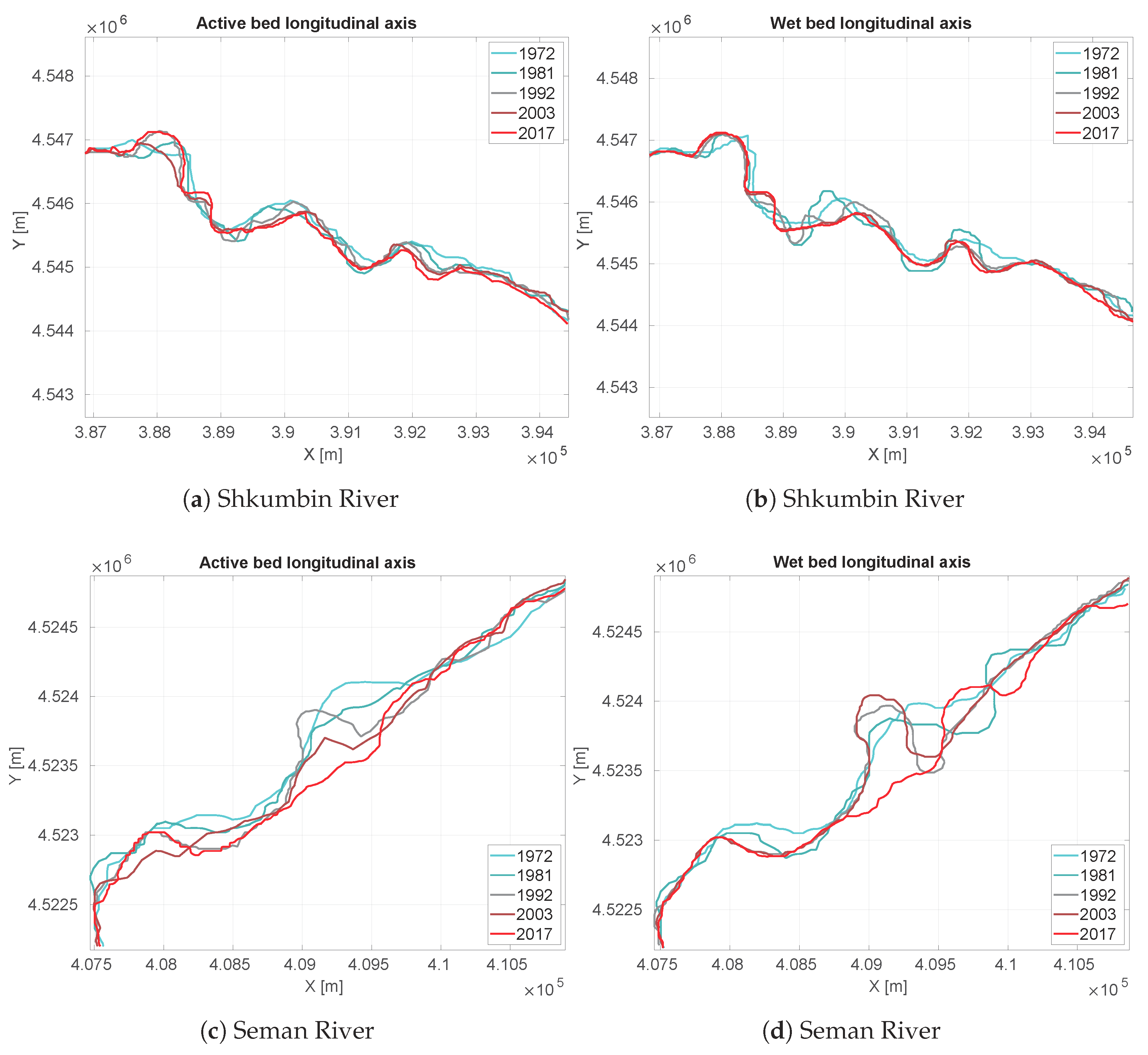
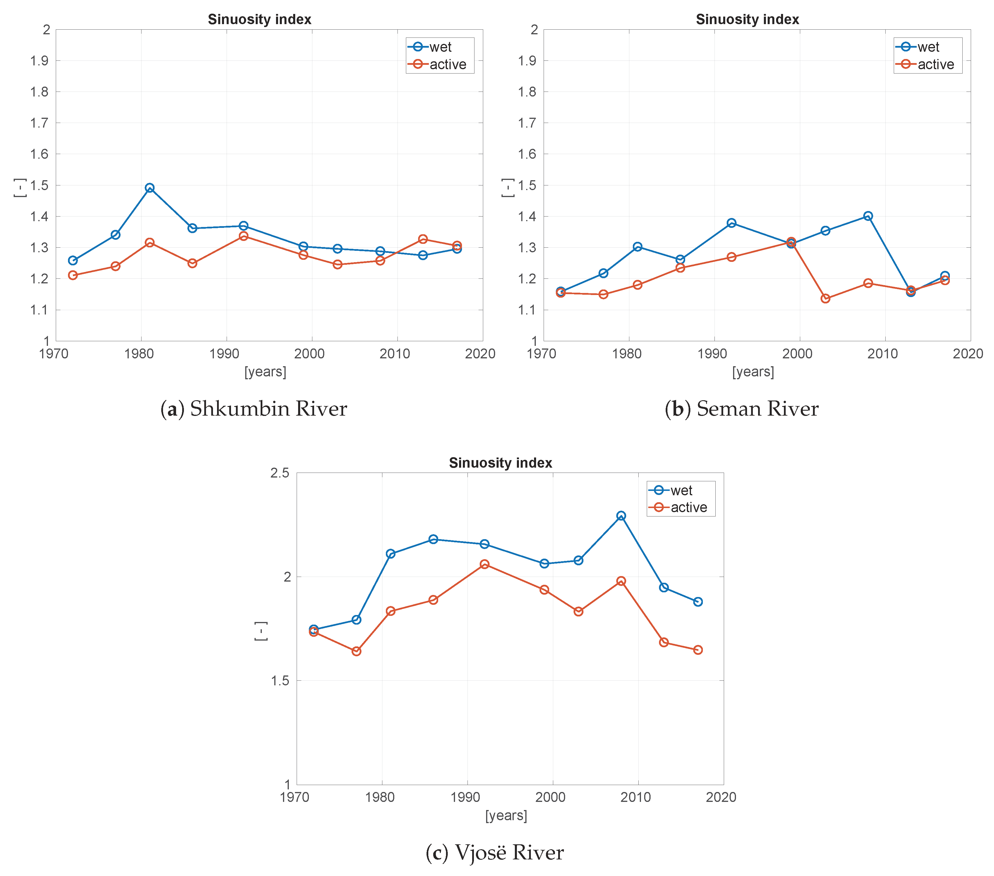
In this work, a semi-automatic image processing procedure is presented to study river hydromorphological evolution on a timescale of several decades. The procedure involves the recognition of river reaches and the extrapolation of morpho-dynamic parameters including: the length and sinuosity index of main river centerlines, wet and active channel widths, surface coverage of water, vegetation and bare sediment units. At first, approximate river centerlines were extracted by processing imagery or DEM data. Active and wet channels were detected by means of a supervised classification of the above-mentioned surface coverage classes. Centerlines were extracted by means of Voronoi diagrams and further processed along with other quantities derived from transects of the surface coverage classified maps. The procedure was applied to a set of data including: DEM, high resolution orthophotos and satellite data from the CORONA, LANDSAT and Sentinel-2 missions. Satellite data cover the time period 1968–2017. The procedure was entirely implemented using free and open source software. Image processing was performed using GRASS (Geographic Resources Analysis Support System). GRASS is a free and open source Geographic Information System (GIS) for geospatial data management and analysis, image processing, graphics’ and maps’ production, spatial modeling and visualization. It is a founding member of the Open Source Geospatial Foundation (OSGeo). Other computations were made by means of ad hoc codes developed in the open source Python programming language.

The study concentrated on three highly dynamic rivers in Albania: the Shkumbin, Seman and Vjosë rivers. The rivers of interest present characteristic traits and marked natural evolution because of the limited anthropic pressures that have occurred over the past decades. Albania represents an area of high interest to investigate rivers’ hydromorphology under near pristine conditions (e.g., the Vjosë river) and their connections with natural (climate) and anthropic stressors, like deforestation, sediment mining in river channels and river regulation from hydropower, which have seen a marked increase in recent years [28]. In addition, Albania represents a paradigmatic case for many emerging contexts where hydromorphological data availability is often limited and where the methodology presented in this work has therefore a high potential for enhancing quantitative knowledge of river forms and processes.

2. Study Site

Though published studies of Albanian rivers date back more than 40 years [29,30,31,32], relatively little information is available on their recent hydromorphological dynamics. Existing studies document the exceptional sediment transport rates of these streams [33]. A comparison of selected Albanian rivers and some other European rivers (

Table 1. Annual total Q_st and unit Q_su sediment loads of selected Albanian and other European rivers [30,33].

River	Qst (${10}^6$ t/Years)	Qsu (t/km${}^2$/Years)
Mat (Albania)	2.5	1034
Shkumbin (Albania)	7.2	2967
Seman (Albania)	16.5	2921
Vjosë (Albania)	8.4	1251
Po (Italy)	13.0	280
Simento (Italy)	4.0	2000
Rhône (France)	31.0	340

) reveals that most Albanian rivers have much higher sediment transport rates per unit catchment area compared to other European rivers in similar climatic settings. This feature is particularly interesting in terms of river hydromorphology, as sediment transport rates represent one of the main control factors driving high rates of morphological activity in rivers [34].

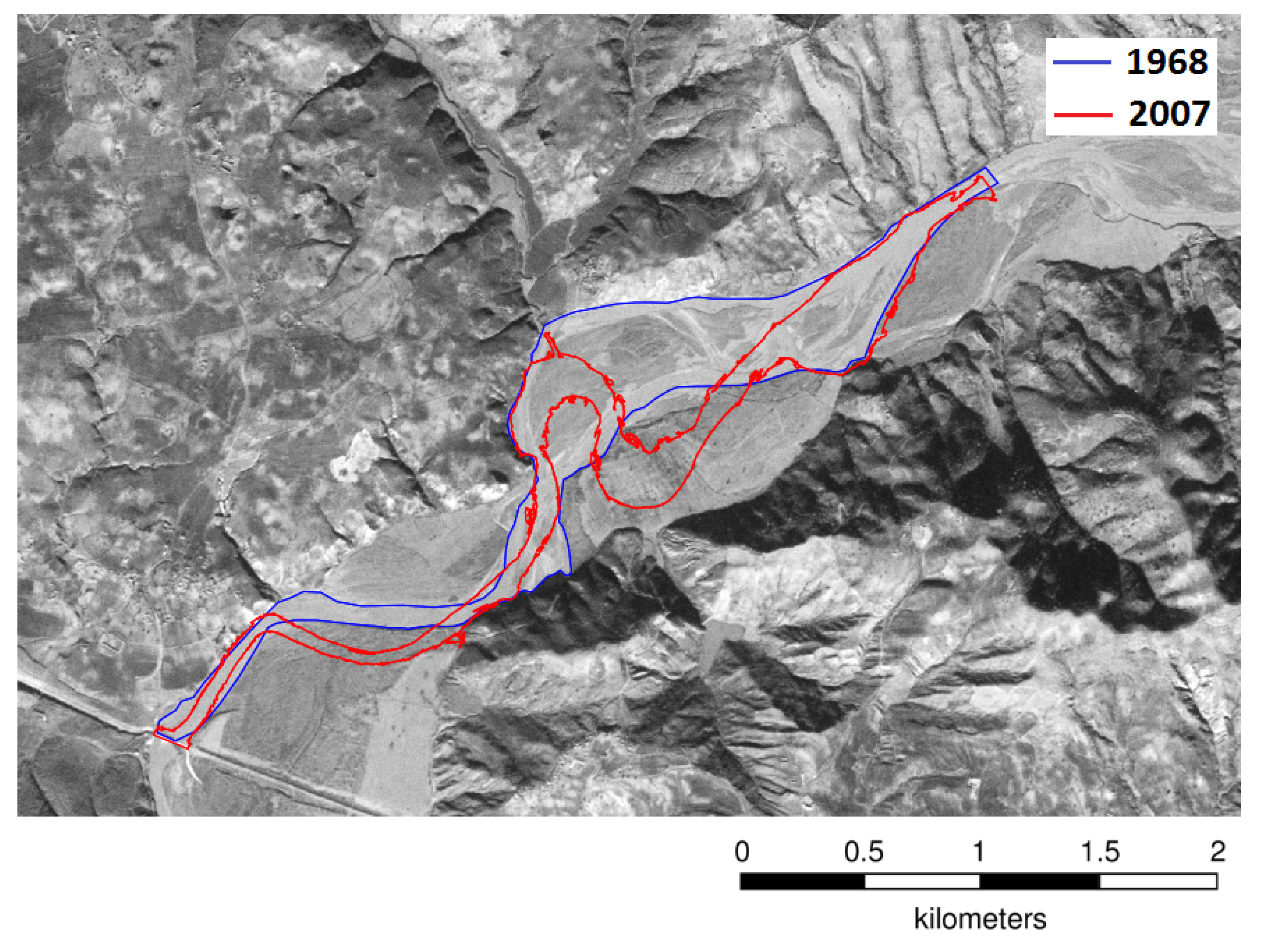
The identification of the river reaches of interest was performed by means of a combined analysis of the entire river course involving both aerial orthophotos and DEM. At first, the DEM was used to extract the river networks and hence to distinguish unconfined, partially-confined and confined reaches. Then, unconfined reaches were selected in order for the analysis to focus on reaches with the highest potential planform dynamics. Among all the identified reaches of potential interest, those presenting the greatest morphological differences between scenes acquired in 1968 and 2007 were selected by means of visual inspection. In the case of the Seman River, a scene centered on a large meander was taken. This meander reached its maximum curvature before a neck cut-off occurred within the study period. For the Vjosë River, a multi-thread section presenting high morphological dynamics was chosen. In the case of the Shkumbin River, a sufficiently extended scene of a single-thread reach in its lower course was attempted.

3. Data

To cover the longest possible time period, several imagery datasets were considered, including: Black and White (BW) images from the 1968 CORONA mission, RGB (Red, Green, Blue) aerial orthophotos from the 2007 Albanian National survey, multi-band LANDSAT imagery from 1972–2017 and 2017 multi-band Sentinel-2 imagery. Details concerning the imagery dataset will follow.

• BW satellite images, 1968: digital scanned copies of photogrammetric BW films acquired in 1968 from one of the first generation of U.S. photo intelligence satellite systems, namely CORONA. Images were originally used by U.S. intelligence agencies and eventually declassified by Executive Order 12,951 in 1995 because of their potential usefulness in global change research. Images used in this study were in part downloaded for free and in part purchased from USGS (United States Geological Survey). The images were acquired in stereo mode by means of a system of two twin cameras named KeyHole (KH) 4A. The spatial resolution was about 2.8 m.
  Mission data: 1049-2 12/22/1968; film IDs: DS1049-2155DA038, DS1049-2155DA042, DS1049-2155DF044, DS1049-2155DF045, DS1049-2155DA045.
• RGB orthophoto, 2007: color orthophotos acquired in 2007. Images were geocoded in WGS84 (World Geodetic System 1984), and coordinates were given in a UTM cartographic plane. Images used in this study were saved from the Albanian State Authority for Geospatial Information (ASIG) portal using WMTS (Web Map Tile Services).
• Multi-band LANDSAT imagery, 1972–2017: a set of multi-band LANDSAT imagery from 1972–2017. Considering the typical time scale of geomorphological phenomena involving natural river systems of interest, a scene every 5–7 years was considered. When possible, and in order to guarantee an acceptable presence of vegetation, scenes within the May–July period were selected. All LANDSAT data were downloaded for free from the Earth-Explorer website.

  Table 2. LANDSAT data.

  Mission	Sensor	Date	ID	Bands
  L-1	MSS	$16/10/1972$	$LM12000321972290AAA04$	B4, B5, B6, B7
  L-2	MSS	$15/03/1977$	$LM22000321977074XXX01$	B4, B5, B6, B7
  L-2	MSS	$03/08/1981$	$LP200R32\_2M19810803$	B4, B5, B6, B7
  L-5	TM+	$11/05/1986$	$LT51860321986131XXX02$	B1, B2, B3, B4
  L-4	TM	$04/06/1992$	$LT41860321992156XXX02$	B1, B2, B3, B4
  L-7	ETM+	$11/08/1999$	$LE71860321999223FUI00$	B1, B2, B3, B4, B8
  L-7	ETM+	$13/07/2003$	$LE71860322003122ASN00$	B1, B2, B3, B4, B8
  L-7	ETM+	$18/07/2008$	$L71186032\_03220080718$	B1, B2, B3, B4, B8
  L-8	OLI	$22/06/2013$	$LC81860322013173LGN00$	B2, B3, B4, B5, B8
  L-8	OLI	$01/06/2017$	$LC81860322017152LGN00$	B2, B3, B4, B5, B8

  contains details concerning LANDSAT data, including mission codes, sensing instruments, acquisition dates and spectral bands used in this work.
• Multi-band Sentinel-2 imagery, 2017: Three tiles of the Level-1C product were considered. Each tile was acquired from the satellite S2A on 11 July 2017, at 9.30 UTC. All data of the COPERNICUS program were downloaded for free from the COPERNICUS HUB website. Bands used in the work had a spatial resolution of 10 m.
• DEM: European DEM provided by EEA (European Environment Agency). The model was a hybrid product based on SRTM and ASTER GDEM data fused by a weighted averaging approach. The spatial resolution was 25 m.

The use of CORONA images was reported by [35,36,37]. However, only recently, some authors have started to work with geometrically-corrected images [38], even if a complete and rigorous procedure to ortho-rectify images was not yet available. In this work, the CORONA images served to establish reference information about river morphological features in order to compare the results of the temporal analysis. To enforce some geometrical improvements on the original uncorrected CORONA images, an ad hoc image rectification was performed estimating the parameters of a local transformation (second order polynomial) with a nearest neighborhood-based resampling. Coordinates of selected Ground Control Points (GCPs) were obtained from the aerial orthophoto. From the hydromorphological point of view, the reaches of the Shkumbin River considered in this study did not present significant differences from the characteristics of the reaches of the Seman and Vjosë rivers. Hence, the analysis based on the CORONA images was carried out only on the reaches of the Seman and Vjosë rivers. In

Table 3. Number of GCPs and Root Mean Square Errors (RMSEs) of the transformation applied to locally rectify CORONAimages.

River	# of GCPs	Max RMSE (m)	Mean RMSE (m)
Seman	15	8.6	6.3
Vjosë	9	3.8	3.1

, the number of GCPs used and statistics about the Root Mean Square Errors (RMSEs) of the transformation are reported.

4. Analysis of Multi-Temporal Imagery Dataset

The adopted procedure was based on the following key steps: (a) identification of an approximate wet channel; (b) identification of a computational region built from the approximate river channel; (c) detection of active and wet channels along with vegetation and gravel coverage units on the active channel; (d) extraction of channel centerlines; (e) extraction of transects of the active and wet channels.

To tackle the differences in the spatial and spectral resolutions of the imagery dataset considered in this work properly, different strategies were developed for the implementation of the previous steps. A schematic description of the choices made for every kind of data is provided at the end of this section. In general, the requirements of user interaction were kept as low as possible to identify the most automated strategies possible. Whenever possible, key steps of the procedure were solved automatically by means of suitable techniques and tools, namely: color space transformation; pan sharpening; thresholding of vegetation and water indices; contextual supervised image classification of false color compositions, RGB and HIS bands; Voronoi diagrams.

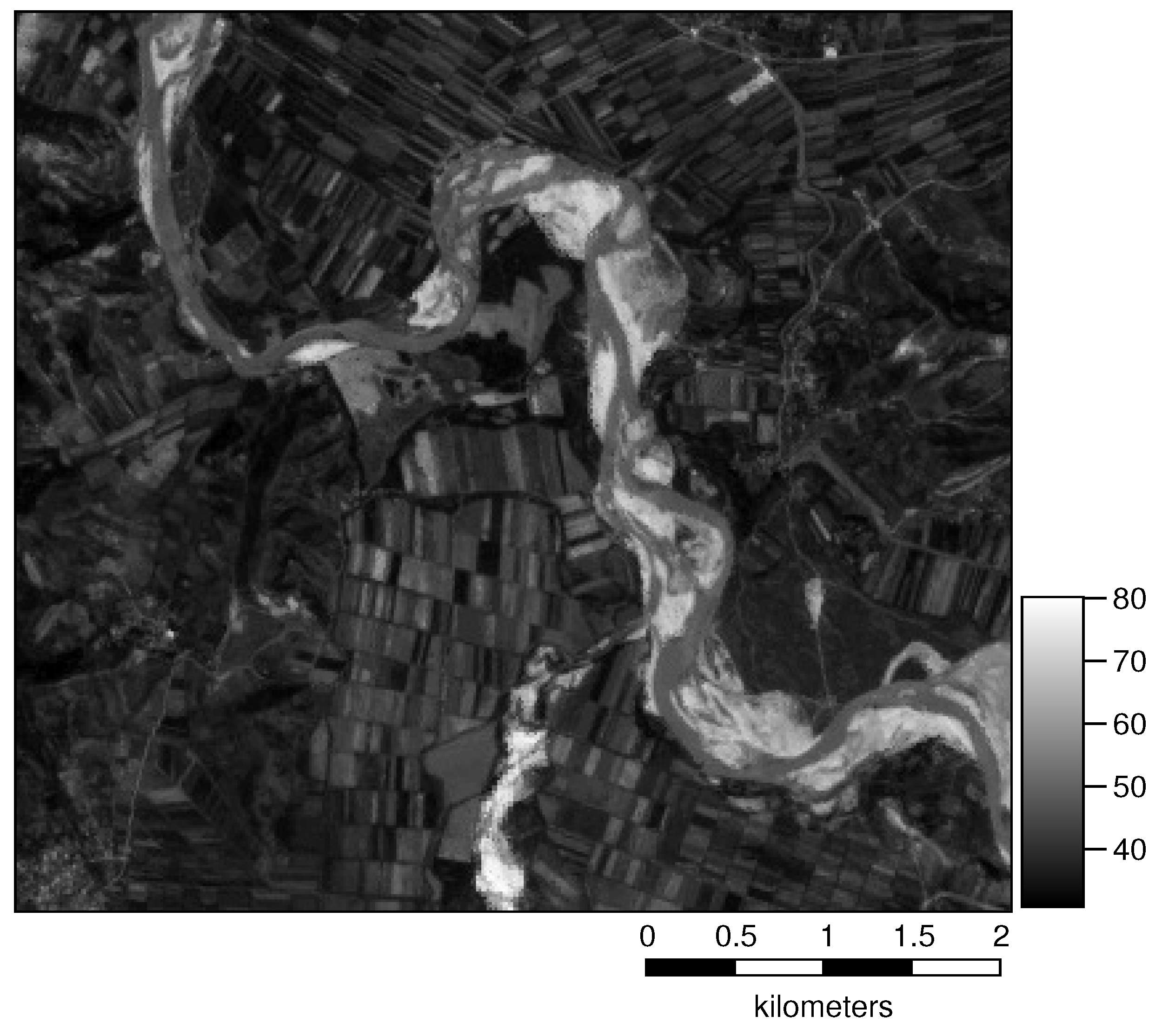
• Color space transformation: The RGB to HSL (Hue, Saturation, Lightness) color transformation was applied to facilitate the detection of the gravel class (see Figure 1). The lightness component of the HSL bands corresponds to the arithmetic mean of the largest and smallest RGB components.
• Pan sharpening: In scenes with LANDSAT 7 or LANDSAT 8 data, i.e., where the panchromatic band is present, pansharpening was performed.
• Thresholding of vegetation and water indices. Plants have a typical absorption/reflection pattern; in fact, chlorophyll strongly absorbs visible light (0.4–0.7 $\mathsf{\mu }$m) for use in photosynthesis, whereas the cell structure of the leaves strongly reflects near-infrared light (from 0.7–1.1 $\mathsf{\mu }$m). The Normalized Difference Vegetation Index (NDVI) is a specific radiometric index that exploits such a typical absorption/reflection pattern, and it is used to map green leaf vegetation. Typically, the NDVI is computed according to the following equation:

  $$\mathrm{NDVI}=\frac{NIR-R}{NIR+R},$$

  (1)

  where $NIR$ and R are the near infra-red and the red bands. NDVI values can range between −1 and +1. However, the typical range of NDVI values is between about −0.1 for non-vegetated surfaces and 0.9 for dense green vegetation canopies. The NDVI increases with increasing green biomass, changes seasonally and responds to favorable, e.g., abundant precipitation, or unfavorable climatic conditions, e.g., drought [39].
  Likewise NDVI, the Normalized Difference Water Index (NDWI) [40] is a radiometric index that exploits a typical absorption/reflection pattern for water mapping purposes. After [41], the NDWI is computed according to the following equation:

  $$\mathrm{NDWI}=\frac{G-NIR}{G+NIR},$$

  (2)

  where G and $NIR$ are the green and the near infra-red bands.
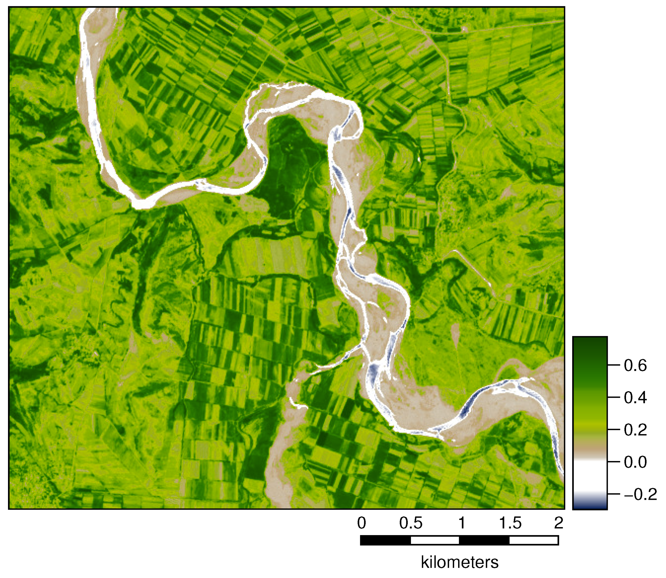
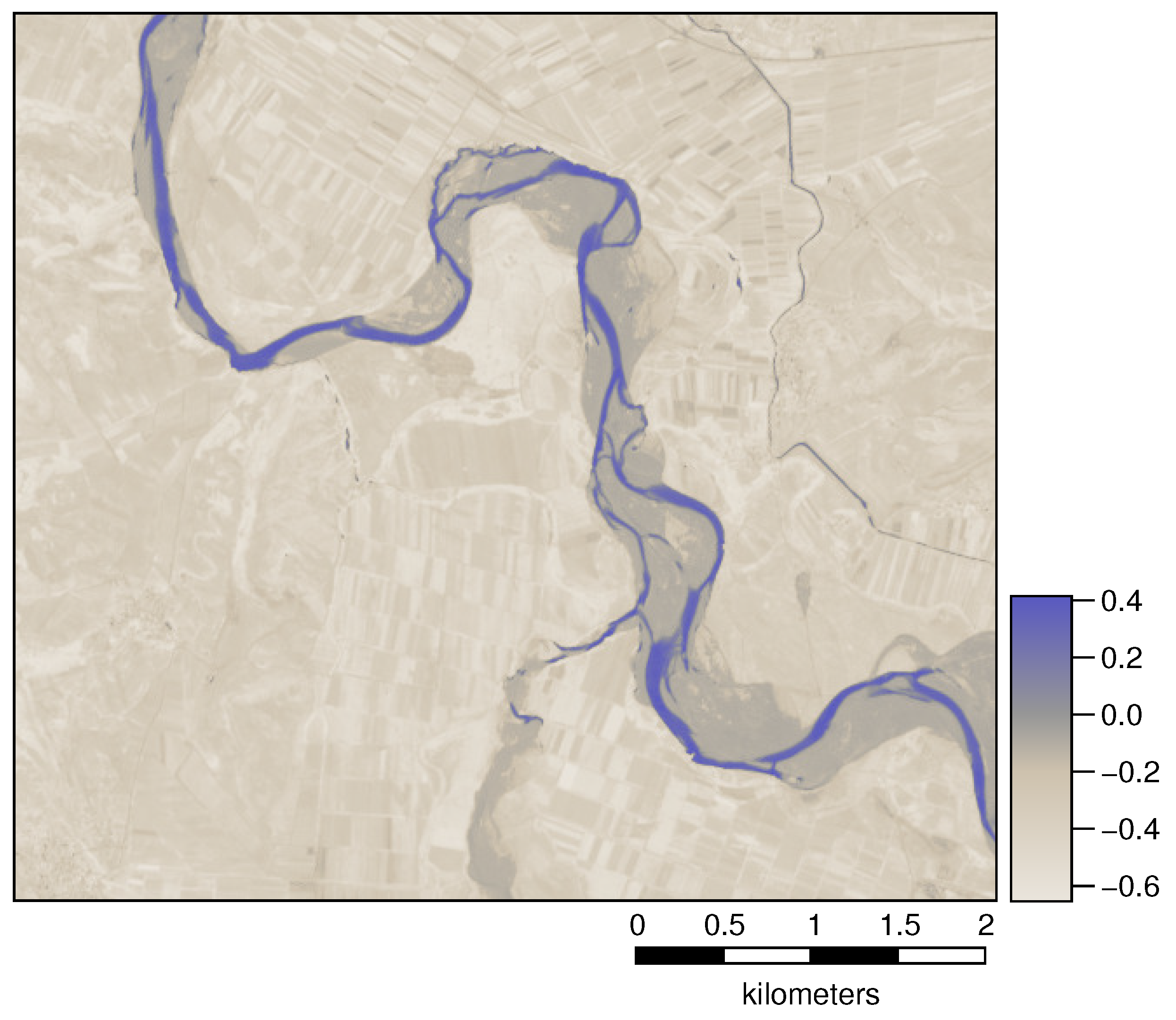
  Thresholds on the NDVI and NDWI maps were set in order to select only pixels corresponding to water. NDVI and NDWI histograms were studied, and pixels with value simultaneously greater than the 90th percentile of the NDWI map and lower than the 10th percentile of the NDVI map were labeled as water pixels. Once the initial water map was obtained, a buffer at a suitable distance was applied to ensure the inclusion of all parts of the wet channel in further processing. Afterwards, the enlarged water map was refined, excluding outside parts of the river reach, such as small pools or secondary channels outside the active channel by means of area thresholding. Likely, the vegetation map was produced selecting pixels with a value greater than the 80th percentile of the NDVI map; the gravel map was produced selecting pixels with a value simultaneously greater than the 95th percentile of the lightness map and lower than the fifth percentile of the saturation map. For every coverage class, the actual percentile values were slightly modified according to the specific imagery dataset considered. Figure 2 and Figure 3 show examples of NDVI and NDWI maps computed from Sentinel-2 imagery.
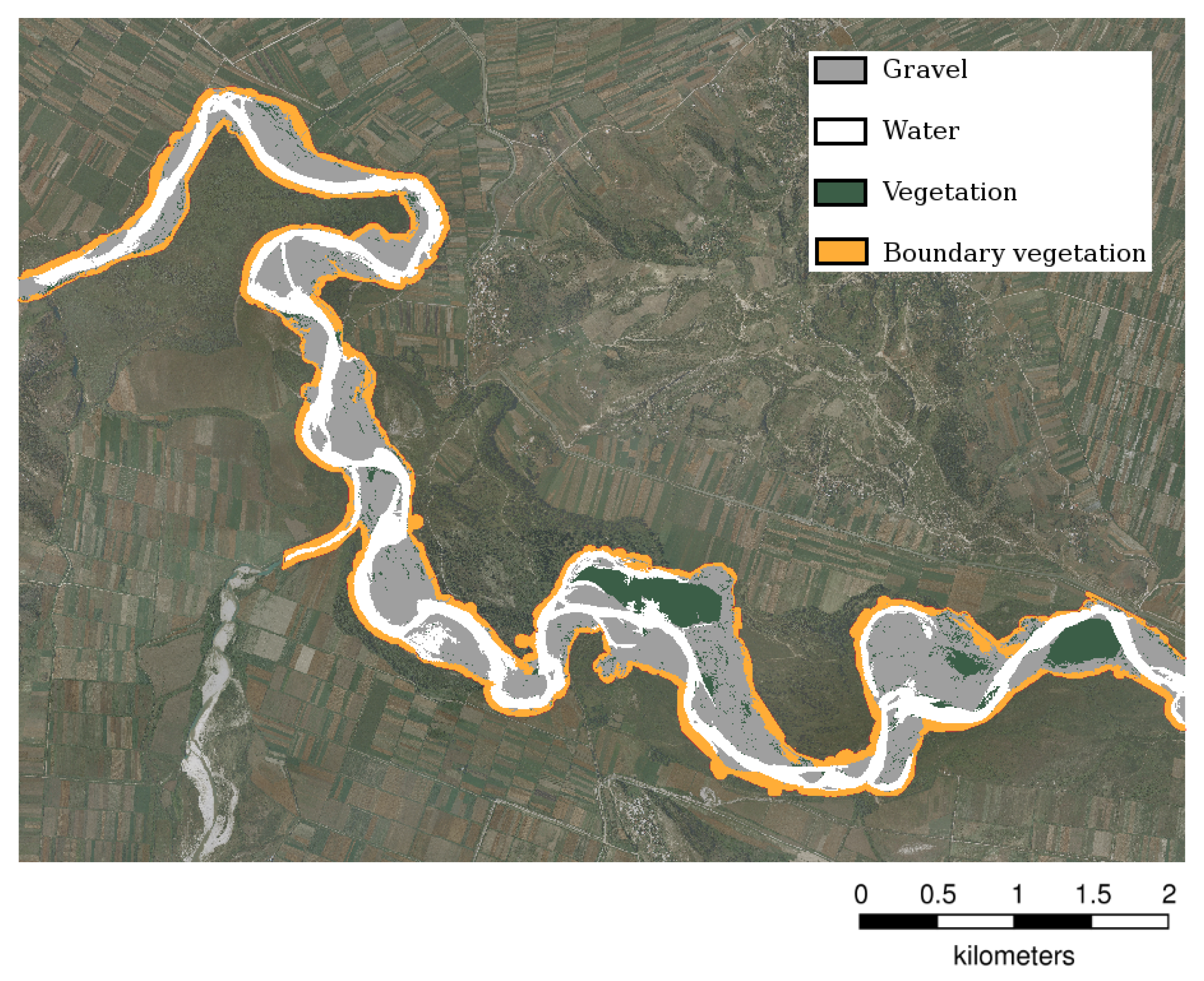
• Contextual supervised image classification: To distinguish surface coverages of different types in multi-spectral imagery, a contextual classifier based on a Sequential Maximum A Posteriori (SMAP) estimation was used. The classifier models a spectral class by means of simple spectral mean and covariance as parameters of a Gaussian mixture distribution. The SMAP segmentation algorithm attempts to improve segmentation accuracy by segmenting the image into regions rather than segmenting each pixel separately. The SMAP algorithm exploits the fact that nearby pixels in an image are likely to have the same class. It works by segmenting the image at various scales or resolutions and using the coarse-scale segmentations to guide the finer scale segmentations. False-color composite maps facilitated the classification of water, vegetation and gravel classes. In Figure 4, an example of the classified coverage units is shown; the orthophoto is used as a background image, and image contrast is reduced in order to enhance readability.
• Voronoi diagrams: The channel centerlines were extracted starting from the Voronoi diagrams of the areas representing the active and wet channels. The centerline is represented by the polyline connecting the centers of all the highest circles inscribed in the Voronoi polygons. In Figure 5, an example of the detected active channel and centerline is shown; the orthophoto is used as a background image, and image contrast is reduced in order to enhance readability.
  From the active channel centerline, lastly, transects were created at a fixed distance of 200 m and with adequate lateral extension. From the channels’ centerlines and the transect sets, hydromorphological parameters were derived by means of an automatic procedure described in Section 5.2.

Specific implementations done to adapt the procedure to different types of data are given hereafter in a step-by-step schematic way.

• BW satellite images: Because of the very limited radiometric content and the reference role of BW images, the procedure, up to the extraction of channel centerlines step, was implemented entirely by hand.
• RGB orthophoto and multi-band LANDSAT 1 and 2 imagery: DEM analysis for the extraction of river axis approximation; buffering approximate axis to limit the area of analysis; RGB to HSI color transformation for thresholding based initial gravel detection; buffering of detected gravel areas for the extraction of active channel; supervised contextual classification of active channel surface coverage; buffering and thresholding for coverage classes refinement; active channel identification after boundary vegetation removal.
• Multi-band LANDSAT 3–8 and Sentinel-2 imagery: NDVI and NDWI analysis for the extraction of river axis approximation; buffering approximate axis to limit the area of analysis; RGB to HSI color transformation for thresholding-based initial gravel detection; buffering of detected gravel areas for the extraction of the active channel; supervised contextual classification of active channel surface coverage; buffering and thresholding for coverage classes refinement; active channel identification after boundary vegetation removal.

5. Results

5.1. Validation of Imagery Analysis Outcomes

• RGB orthophoto: Validation was performed against reference maps obtained by manual digitalization after expert visual inspection of the entire reaches set. Hydromorphological reference parameters were hence computed starting from the reference maps. The production of the reference maps took a couple of days.

  Table 4. Mean and standard deviation of the differences between the active channel widths obtained from the applied procedure and from the reference maps.

  River	Reach	Mean (m)	Std. Dev. (m)
  Shkumbin	1	−0.7	7.0
  	2	32.7	22.9
  Seman	1a	1.6	8.7
  	1b	1.5	5.1
  	2	4.4	8.4
  	3	6.7	31.7
  Vjosë	1	−2.8	14.4
  	2	−6.1	25.0
  	3	10.0	37.4

  shows the mean and the standard deviation of the differences between the active channel widths obtained from the applied procedure and from the reference maps. Values were, in general, lower than 10 m and had a percentage difference below 5%. Because of radiometric ambiguities between pixels of different coverage classes and the hard classification of mixed pixels, standard deviations presented greater values and variability.
• Multi-band LANDSAT and Sentinel-2 imagery: Regarding the processing of LANDSAT data, it was noted that parts of the scene that did not belong to the river channel were still inserted into the final map, despite carefully-chosen threshold values. This occurred in the areas adjacent to the river where gravel roads or quarries were present, or simply vegetation-free areas that were wrongly classified as gravel. Other times, vegetation-rich river portions were not included in the final map because of the removal of boundary vegetation. To fix these problems, when available data made it possible, a refinement step was set up. The refinement step was based on the application of the standard procedure on two scenes belonging to the same year, but in different seasons. In the summer standard scene, the vegetation recognition threshold was lowered, so that the classification of the other two classes was reduced to the minimum. The water class recognition threshold was modified accordingly to avoid distortion. A map of the active channel was obtained where the vegetation was predominant and the gravel parts were partially filtered. This first new map helped in solving the problem of incorrect classification of quarries and of other gravel disturbances adjacent to the river. Then, for the same river, a late autumn or winter scene of the same year was selected. The standard procedure was applied to produce a map in which, for seasonal issues, vegetation was poor and the gravel class was increased. This map typically improved the contour outlines of the river channel areas where summer vegetation led classification disturbances. This second map helped in solving the problem of incorrect classification of parts of the river that in summer were covered by vegetation and thus excluded from the first map. The maps were therefore intersected, and the result were used to cut the initial map of the procedure. In this way, a final active channel classification included all significant parts of the scene. Validation was performed against hydromorphological reference parameters derived from manual digitalization of RGB color maps.

  Table 5. Comparison between the outputs of the applied procedure and values from manual digitalization, Vjosë River.

  Parameters		Applied Procedure (AP)	Manual Digitalization (HD)	$\Delta$ (HD−AP)	% $\Delta$
  $W^{act}$	(m)	316	329	+13	+4
  $W^{wet}$	(m)	94	96	+2	+2.3
  $L^{act}$	(m)	9304	9622	+318	+3.4
  $I_s^{act}$	(-)	1.65	1.70	+0.05	+3.03
  $L^{wet}$	(m)	10,969	11,586	+617	+5.6
  $I_s^{wet}$	(-)	1.88	1.99	+0.11	+5.85

  shows the results of the validation process for the Vjosë River. Overall, percentage differences between length and width values obtained from the applied procedure and from the reference maps were below 6%. Again, differences were mainly due to radiometric ambiguities between pixels of different coverage classes and the hard classification of mixed pixels. In cases where it was not possible to apply the refinement procedure, maps were refined manually. Comparable results were obtained for the rivers Seman and Shkumbin.

5.2. Characterization of River Morphology

From the channel centerlines extracted through the image processing procedure described in Section 4, channel centerline lengths, sinuosity indices and widths were extracted. Hydromorphological parameters were computed for all the scenes considered in this work to study the parameter variations over time. The sinuosity index was computed as the ratio between the channel centerline length and the distance between the starting and the ending points of the channel. From the transects, the mean, maximum and minimum widths were computed. For every reach, the percentage distribution of the surface coverage classes was computed.

• RGB orthophoto:

  Table 6. Coverage classes distribution, active channel widths and standard deviations, active channel areas, number of transects, channel centerline lengths, sinuosity indices and fluvial reaches classification obtained from the processing of the 2007 aerial orthophotos.

  River	Reach	Classes (%)			Area (km2)	Widths (m)				# Transects	Lengths (m)	Sinuosity Index	Type
  		Water	Gravel	Vegetation		Mean	Min	Max	Std. Dev.
  Shkumbin	1	50.2	42.4	7.4	0.94	49.6	18.4	129.6	21.1	83	16,775	1.84	single-thread
  	2	8.7	76.1	15.2	3.59	351.4	111.6	816.2	162.7	42	8669	1.15	multi-thread/transitional
  Seman	1a	44.4	52.6	2.9	0.98	89.7	48.6	281.0	39.8	47	9556	1.76	single-thread
  	1b	68.2	28.3	3.5	0.25	40.8	20.2	77.2	12.3	30	6153	1.78	single-thread
  	2	34.4	45.8	19.8	0.58	100.9	40.6	279.4	63.8	24	5358	1.30	multi-thread/transitional
  	3	10.4	69.1	20.5	2.92	361.4	169.4	705.8	112.3	38	7633	1.09	multi-thread/transitional
  Vjosë	1	58.0	35.3	6.7	1.81	130.5	52.0	378.0	64.9	60	12,207	1.60	single-thread
  	2	35.9	53.2	10.9	3.99	271.9	76.6	686.6	146.8	65	13,303	1.75	multi-thread/transitional
  	3	23.1	67.3	9.6	4.99	406.8	183.6	668.2	123.7	50	10,628	1.11	multi-thread/transitional

  shows coverage classes’ distribution, active channel widths and standard deviations, active channel areas, number of transects, channel centerline lengths, sinuosity indices and fluvial reaches’ classification obtained from the processing of the 2007 aerial orthophotos. From the coverage classes- distribution, two states can be distinguished: (1) the wet area was close to or greater than the gravel area, and the vegetation was very scarce; (2) the wet area was less than the gravel area, and vegetation area was not negligible. Differences in widths (between mean, minimum and maximum values) and standard deviations, when jointly considered, permitted distinguishing reaches with respect to different fluvial typologies: single-thread reaches presented low mean widths and variations with respect to transitional or multi-thread reaches. The sinuosity indices were all greater than 1.05, as expected for natural reaches [18].
• Multi-band LANDSAT and Sentinel-2 imagery. In

  Table 7. Cartesian (${·}_{cx}$) and axial (${·}_{ax}$) lengths (L), sinuosity index (I) of active (${·}^{ab}$) and wet (${·}^{wb}$) channels, extracted from the elaboration of the Vjosë River LANDSAT imagery, time period 1972–2017.

  	${{\mathit{L}}_{\mathit{cx}}}^{\mathit{ab}}$	${{\mathit{L}}_{\mathit{ax}}}^{\mathit{ab}}$	${{\mathit{L}}_{\mathit{cx}}}^{\mathit{wb}}$	${{\mathit{L}}_{\mathit{ax}}}^{\mathit{wb}}$	${{\mathit{I}}_{\mathit{s}}}^{\mathit{ab}}$	${{\mathit{I}}_{\mathit{s}}}^{\mathit{wb}}$
  	(m)	(m)	(m)	(m)	(-)	(-)
  1972	5749	9966	5832	10,180	1.73	1.75
  1977	5830	9560	5882	10,539	1.64	1.79
  1981	5850	10,729	5673	11,969	1.83	2.11
  1986	5663	10,688	5562	12,121	1.89	2.18
  1992	5484	11,294	5533	11,931	2.06	2.16
  1999	5598	10,841	5652	11,656	1.94	2.06
  2003	5587	10,232	5679	11,799	1.83	2.08
  2008	5643	11,165	5653	12,961	1.98	2.29
  2013	5609	9440	5700	11,099	1.68	1.95
  2017	5650	9304	5840	10,969	1.65	1.88

  ,

  Table 8. Cartesian (${·}_{cx}$) and axial (${·}_{ax}$) lengths (L), sinuosity index (I) of active (${·}^{ab}$) and wet (${·}^{wb}$) channels, extracted from the elaboration of the Shkumbin River LANDSAT imagery, time period 1972–2017.

  	${{\mathit{L}}_{\mathit{cx}}}^{\mathit{ab}}$	${{\mathit{L}}_{\mathit{ax}}}^{\mathit{ab}}$	${{\mathit{L}}_{\mathit{cx}}}^{\mathit{wb}}$	${{\mathit{L}}_{\mathit{ax}}}^{\mathit{wb}}$	${{\mathit{I}}_{\mathit{s}}}^{\mathit{ab}}$	${{\mathit{I}}_{\mathit{s}}}^{\mathit{wb}}$
  	(m)	(m)	(m)	(m)	(-)	(-)
  1972	7983	9664	8243	10,368	1.21	1.26
  1977	8037	9963	8264	11,074	1.24	1.34
  1981	7512	9881	8201	12,227	1.32	1.49
  1986	7982	9968	8209	11,176	1.25	1.36
  1992	8022	10,720	8252	11,299	1.34	1.37
  1999	8005	10,210	8263	10,766	1.28	1.30
  2003	7977	9933	8257	10,698	1.25	1.30
  2008	7952	9999	8242	10,613	1.26	1.29
  2013	8000	10,613	8255	10,523	1.33	1.27
  2017	8022	10,472	8267	10,710	1.31	1.30

  and

  Table 9. Cartesian (${·}_{cx}$) and axial (${·}_{ax}$) lengths (L), sinuosity index (I) of active (${·}^{ab}$) and wet (${·}^{wb}$) channels, extracted from the elaboration of the Seman River LANDSAT imagery, time period 1972–2017.

  	${{\mathit{L}}_{\mathit{cx}}}^{\mathit{ab}}$	${{\mathit{L}}_{\mathit{ax}}}^{\mathit{ab}}$	${{\mathit{L}}_{\mathit{cx}}}^{\mathit{wb}}$	${{\mathit{L}}_{\mathit{ax}}}^{\mathit{wb}}$	${{\mathit{I}}_{\mathit{s}}}^{\mathit{ab}}$	${{\mathit{I}}_{\mathit{s}}}^{\mathit{wb}}$
  	(m)	(m)	(m)	(m)	(-)	(-)
  1972	4219	4869	4207	4873	1.15	1.16
  1977	4255	4890	4169	5073	1.15	1.22
  1981	4266	5033	4240	5521	1.18	1.30
  1986	4235	5227	4229	5332	1.23	1.26
  1992	4229	5367	4279	5898	1.27	1.38
  1999	4293	5658	4288	5624	1.32	1.31
  2003	4289	4871	4283	5797	1.14	1.35
  2008	4246	5032	4219	5910	1.19	1.40
  2013	4244	4931	4212	4870	1.16	1.16
  2017	4229	5050	4163	5032	1.19	1.21

  , the lengths of each river reach per year of study are reported. Subsequently, in order to visualize the time evolution of the watercourses, the planimetric patterns of some selected centerlines of active and wet river channel for the three rivers are plotted in Figure 6a–f. Alongside the centerline plots in Figure 7a–c and Figure 8a–f, the plots of the temporal variations of the sinuosity index and of the wet and active channel widths are also presented. Observing the charts of the centerlines, it can be seen how some meanders evolved over time, changing their curvature and moving both laterally and longitudinally. In the case of the Seman River, a large meander that reached its peak in 2008 and then underwent a cut-off, is visible; see Figure 9. The progressive growth and consequential cut-off of the meander in the Seman River scene is also visible in the chart of active channel lengths. The highest values of the sinuosity indices appeared in the case of the Vjosë River, which showed peak values of about 2.3 in 2008.
  In this work, Sentinel-2 data were basically considered for comparison with respect to LANDSAT 8 to support a further application of the presented procedure in a real-time river monitoring system based on a rolling processing mechanism. Satellite-2A was acquired on 11 July 2017, and LANDSAT 8 data were acquired almost at the same time on 1 June 2017. Outcomes of the application of the procedure to the Sentinel-2 data of the Vjosë River are presented in the

  Table 10. Comparison of the results obtained with LANDSAT-8 and Sentinel-2 imagery of the Vjosë River, sensed in the summer of 2017; active (${·}^{ab}$) and wet (${·}^{wb}$) channel widths, Cartesian (${·}_{cx}$) and axial (${·}_{ax}$) lengths (L) and sinuosity indexes (I).

  Parameters	LANDSAT-8	Sentinel-2	$\Delta$ (S2−L8)	% $\Delta$
  $W_{ab}$ (m)	316	305	−11	−3.5
  $W_{wb}$ (m)	94	62	−32	−34
  ${L_{cx}}^{ab}$ (m)	5650	5649	−1	-
  ${L_{ax}}^{ab}$ (m)	9304	9338	+34	+0.4
  ${I_s}^{ab}$ (−)	1.65	1.65	-	-
  ${L_{cx}}^{wb}$ (m)	5840	5861	+21	+0.4
  ${L_{ax}}^{wb}$ (m)	10,969	11,073	+104	+0.9
  ${I_s}^{wb}$ (-)	1.89	1.89	-	-

  . The results of the Sentinel-2 data processing differed very little from those obtained from the LANDSAT 8 data. The average wet channel mean width ($W_{wb}$) was an exception. The value obtained from the Sentinel-2 data was 33% lower than the value derived from LANDSAT 8 data. In fact, the extent of the wet channel can be easily affected by the rainfall. Investigation of such a relevant difference was performed on the basis of rainfall data acquired at a weather station located near Vorë, a coastal city located within the Vjosë River basin. According to the records, significant rainfall events occurred in May 2017, just a few days before the acquisition of the LANDSAT 8 imagery.
• RGB orthophotos and BW CORONA: Another comparison was carried out between the results obtained from the processing of the 2007 RGB orthophotos and those of the 1968 BW images from the CORONA satellite mission. The two datasets have the highest spatial resolutions of the entire image dataset considered in this work, respectively 0.2 and 2.8 m. The comparison was conducted on two reaches of the rivers Seman and Vjosë. Figure 10 and Figure 11 show the compared regions in the 1968 and 2007 images, respectively.

  Table 11. Hydromorphological parameters derived from historical images and orthophotos, rivers Seman and Vjosë.

  River	Year	Widths (m)			Lengths (m)	Sinuosity Index
  		Mean	Min	Max
  Seman	1968	187.2	436	436.2	4445	1.12
  	2007	100.9	406	279.4	15,358	1.30
  Vjosë	1968	430.3	658	1792.4	11,494	1.51
  	2007	271.6	766	686.6	13,303	1.75

  shows the values of hydromorphological parameters derived from the historical images and those derived from the orthophotos, as already reported in Table 6.
  The sinuosity indices and the channel widths changed significantly. Mean and maximum widths showed greater differences, whereas smaller differences were found for the minimum width. Mean widths decreased by about 36% and 46% for the Vjosë and Seman reaches, respectively.

6. Discussion and Future Prospects

We discuss the outcomes of the present work at two levels: first at a technical, methodological level and then in relation to its broader significance for fluvial processes and related environmental implications for the examined case studies in Albania.

The proposed procedure proved to be a valid and effective tool to map river morphology and its temporal change. In particular, the extraction of centerlines, as well as active and wet channel width was sufficiently accurate, with differences with respect to the manual measurements below 6%. Moreover, the comparison with high resolution data (Sentinel-2) confirmed the accuracy of the results obtained by the Landsat imagery. Overall, the validation did not show any particular problem in the semi-automatic processing.

As satellite data were acquired by different sensors over a 40-year period, threshold values for radiometric indices were set specifically in order to account for different light conditions, the seasonality of the scenes and differences in spatial and spectral resolutions. The procedure provided high quality results for scenes obtained from the images acquired in the period 1986–2017, i.e., those with a spatial resolution of 30 and 15 m. As for the 1972–1981 data, the estimation of widths was affected by the relatively low spatial accuracy (about 60 m) of the scenes. However, the results obtained from the processing of CORONA images did not differ too much from those obtained from the processing of historical data. In the first years considered in this study, scenes were few in number and often in bad condition. In these cases, the homogeneity of the data concerning seasonality is lacking.

The general quality of the results and, in a particular way, the notable agreement between the outcomes derived from Sentinel-2 and LANDSAT 8 data prompt further applications of the procedure to entire river systems. Moreover, the high acquisition frequency of recent satellite missions offers the opportunity to implement rolling monitoring systems.

The proposed procedure exploits open data and is implemented by means of free and open source software. Such conditions can have great relevance for the application of the proposed methodology to those contexts where the availability of historical and recent environmental data is limited or of fragmented quality. This is the case, in general, of emerging or developing countries where rapid environmental changes driven by socio-economic development are presently occurring and expected in the near future.

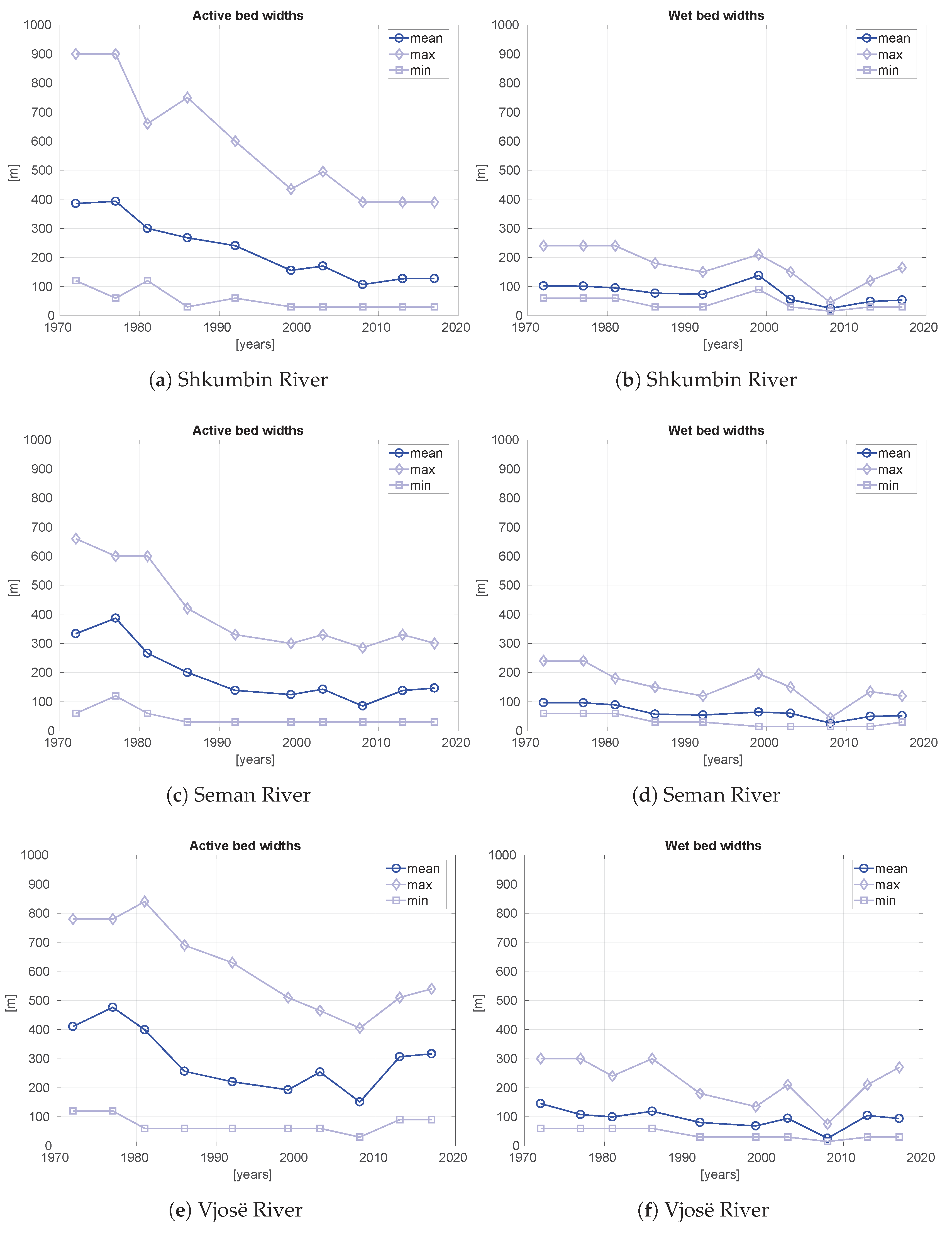
In the specific case of the three examined Albanian rivers, one of the main outcomes of the analysis is that all the studied river reaches reduced their width, although at a different rate. The Vjosë River seems to be the least affected by this narrowing process, possibly thanks to its greater dynamism over time. The Seman and Shkumbin rivers experienced a remarkable channel narrowing, considering both the wet and even more the active width. They reduced their active width (mean value) to half or even one third of the value observed in 1972. This behavior is similar to what was observed for many other European rivers [42], and in particular for many Italian rivers [43]. Reduction of the active channel width can have dramatic consequences for a variety of aquatic, riparian and terrestrial ecosystems, which have direct or indirect legacies in relation to the morphological functioning of the river corridor [44]. For instance, when the active river corridor width is reduced, the surface available for bare sediments and instream habitats is largely replaced by permanently-vegetated surfaces, which may impact entire bird communities that rely on bare sediment surfaces for nesting and incubation [45] and fish communities that need to adapt to heavily-modified hydromorphological conditions [46]. When habitat reduction exceeds a threshold, adaptation to the new river condition may no longer be possible, with potentially dramatic consequences in terms of biodiversity loss [47]. Narrowing of the active river corridor may also negatively affect the hydraulic safety of human communities with respect flooding risk, because a narrowed river corridor determines higher water levels during floods. River narrowing is also often accompanied by riverbed incision [48], which has often resulted in much increased damage for river structures like bridges, levees and check dams.

River width variability has often been observed at relatively slow time scales (decades [48]), and it is therefore very important to develop tools that allow tracking such changes over the relevant time scales, and across a variety of geographical contexts characterized by different paths of data source availability. A complementary ingredient for effective environmental management would be to understand the causes and controls of those evolutionary river trajectories. Broadly speaking, the decrease of active channel width has been explained by the concurrent effect of different factors, including climate change, land use change, dam construction and in-channel gravel mining [49]. The present study does not attempt to account for the causality of the observed changes on the selected Albanian rivers; for this, further research is needed. Here, we demonstrate that the developed procedure allows the collection of relevant data to reconstruct such changes in the river morphological trajectories. The ability to automatically detect the river planform at the catchment (or regional) scale is a first essential step towards effective management of such sensitive and dynamic landscape elements, within a broader perspective of environmental sustainability.

Future developments of the present work are both at a methodological level and in relation to its high potential for enhanced information acquisition on the temporal fluvial dynamics. From a technical point of view, the procedure could be improved or expanded by applying super resolution algorithms that could improve in a particular way the analysis of low resolution data [50]. The CORONA images could be ortho-rectified to improve the metric information obtained from the processing of those data, thus greatly expanding the temporal window on which close multi-temporal comparisons are feasible. At the level of fluvial process understanding, of particular interest are applications of the proposed methodology to emerging or developing contexts where large river exploitation is planned at a global level [51]. Integration with the analysis of the main anthropic and climatic controlling factors of river morphological evolution can provide a high added value for sustainable river management.

References

1. Righini, M.; Surian, N. Remote Sensing as a Tool for Analysing Channel Dynamics and Geomorphic Effects of Floods. In Flood Monitoring through Remote Sensing; Springer: Berlin, Germany, 2018. [Google Scholar]
2. Carbonneau, P.; Piégay, H. (Eds.) Fluvial Remote Sensing for Science and Management; Wiley-Blackwell: Hoboken, NJ, USA, 2012. [Google Scholar]
3. Demarchi, L.; Bizzi, S.; Piégay, H. Regional hydromorphological characterization with continuous and automated remote sensing analysis based on VHR imagery and low-resolution LiDAR data. Earth Surf. Process. Landf. 2017, 42, 531–551. [Google Scholar] [CrossRef] [Green Version]
4. Sundermann, A.; Stoll, S.; Haase, P. River restoration success depends on the species pool of the immediate surroundings. Ecol. Appl. 2011, 21, 1962–1971. [Google Scholar] [CrossRef] [PubMed]
5. Poppe, M.; Kail, J.; Aroviita, J.; Stelmaszczyk, M.; Gielczewski, M.; Muhar, S. Assessing restoration effects on hydromorphology in European mid-sized rivers by key hydromorphological parameters. Hydrobiologia 2016, 769, 21–40. [Google Scholar] [CrossRef]
6. Piégay, H.; Mathias, K.G.; Sear, D.A. Integrating geomorphological tools to address practical problems in river management and restoration. In Tools in Fluvial Geomorphology; Wiley-Blackwell: Hoboken, NJ, USA, 2016. [Google Scholar]
7. Marteau, B.; Vericat, D.; Gibbins, C.; Batalla, R.J.; Green, D.R. Application of Structure from Motion photogrammetry to river restoration. Earth Surf. Process. Landf. 2017, 42, 503–515. [Google Scholar] [CrossRef]
8. Parasiewicz, P. Using MesoHABSIM to develop reference habitat template and ecological management scenarios. River Res. Appl. 2007, 23, 924–932. [Google Scholar] [CrossRef]
9. Conallin, J.; Boegh, E.; Jensen, K.J. Instream physical habitat modelling types: An analysis as stream hydromorphological modelling tools for EU water resource managers. Int. J. River Basin Manag. 2010, 8, 93–107. [Google Scholar] [CrossRef]
10. Bergeron, N.; Carbonneau, P.E. Geosalar: Innovative Remote Sensing Methods for Spatially Continuous Mapping of Fluvial Habitat at Riverscape Scale. In Fluvial Remote Sensing for Science and Management; John Wiley & Sons: Hoboken, NJ, USA, 2012; Chapter 9; pp. 193–213. [Google Scholar]
11. Demarchi, L.; Bizzi, S.; Piégay, H. Hierarchical object-based mapping of riverscape units and in-stream mesohabitats using LiDAR and VHR Imagery. Remote Sens. 2016, 8, 97. [Google Scholar] [CrossRef] [Green Version]
12. Belletti, B.; Rinaldi, M.; Bussettini, M.; Comiti, F.; Gurnell, A.M.; Mao, L.; Nardi, L.; Vezza, P. Characterising physical habitats and fluvial hydromorphology: A new system for the survey and classification of river geomorphic units. Geomorphology 2017, 283, 143–157. [Google Scholar] [CrossRef]
13. Poole, G.C. Stream hydrogeomorphology as a physical science basis for advances in stream ecology. J. N. Am. Benthol. Soc. 2010, 29, 12–25. [Google Scholar] [CrossRef]
14. Elosegi, A.; Díez, J.; Mutz, M. Effects of hydromorphological integrity on biodiversity and functioning of river ecosystems. Hydrobiologia 2010, 657, 199–215. [Google Scholar] [CrossRef]
15. Legleiter, C.J.; Marcus, W.A.; Lawrence, R.L. Effects of sensor resolution on mapping instream habitats. Photogramm. Eng. Remote Sens. 2002, 68, 801–807. [Google Scholar]
16. Neal, J.C.; Bates, P.D.; Fewtrell, T.J.; Hunter, N.M.; Wilson, M.D.; Horritt, M.S. Distributed whole city water level measurements from the Carlisle 2005 urban flood event and comparison with hydraulic model simulations. J. Hydrol. 2009, 368, 42–55. [Google Scholar] [CrossRef]
17. Bizzi, S.; Demarchi, L.; Grabowski, R.C.; Weissteiner, C.J.; Van de Bund, W. The use of remote sensing to characterise hydromorphological properties of European rivers. Aquat. Sci. 2016, 78, 57–70. [Google Scholar] [CrossRef] [Green Version]
18. Rinaldi, M.; Belletti, B.; Bussettini, M.; Comiti, F.; Golfieri, B.; Lastoria, B.; Marchese, E.; Nardi, L.; Surian, N. New tools for the hydromorphological assessment and monitoring of European streams. J. Environ. Manag. 2017, 202, 363–378. [Google Scholar] [CrossRef] [PubMed]
19. Mitidieri, F.; Papa, M.N.; Amitrano, D.; Ruello, G. River morphology monitoring using multitemporal SAR data: Preliminary results. Eur. J. Remote Sens. 2016, 49, 889–898. [Google Scholar] [CrossRef]
20. Vijith, H.; Dodge-Wan, D. Morphology and channel characteristics of an equatorial tropical river in Malaysian Borneo: A detailed evaluation through spatially explicit geomorphometric modelling. Model. Earth Syst. Environ. 2018, 4, 325–337. [Google Scholar] [CrossRef]
21. Henshaw, A.J.; Gurnell, A.M.; Bertoldi, W.; Drake, N.A. An assessment of the degree to which landsat TM data can support the assessment of fluvial dynamics, as revealed by changes in vegetation extent and channel position, along a large river. Geomorphology 2013, 202, 74–85. [Google Scholar] [CrossRef]
22. Belletti, B.; Dufour, S.; Piégay, H. Regional variability of aquatic pattern in braided reaches (example of the French Rhône basin). Hydrobiologia 2013, 712, 25–41. [Google Scholar] [CrossRef]
23. Clerici, A.; Perego, S. A set of GRASS GIS-based Shell scripts for the calculation and graphical display of the main morphometric parameters of a river channel. Int. J. Geosci. 2016, 7, 135–143. [Google Scholar] [CrossRef]
24. Cencetti, C.; De Rosa, P.; Fredduzzi, A. Geoinformatics in morphological study of River Paglia, Tiber River basin, Central Italy. Environ. Earth Sci. 2017, 76, 128. [Google Scholar] [CrossRef]
25. Gilvear, D.; Bryant, R. Analysis of remotely sensed data for fluvial geomorphology and river science. In Tools in Fluvial Geomorphology; Wiley-Blackwell: Hoboken, NJ, USA, 2016; pp. 103–132. [Google Scholar]
26. Geerling, G.W.; Vreeken–Buijs, M.J.; Jesse, P.; Ragas, A.M.J.; Smits, A.J.M. Mapping river floodplain ecotopes by segmentation of spectral (CASI) and structural (LiDAR) remote sensing data. River Res. Appl. 2009, 25, 795–813. [Google Scholar] [CrossRef]
27. Wiederkehr, E.; Dufour, S.; Piégay, H. Localisation et caractérisation des géomorphosites fluviaux à l’échelle des réseaux hydrographiques, exemples d’applications géomatiques dans le bassin de la Drôme. Géomorphol. Relief Processus Environ. 2010, 2, 175–188. [Google Scholar] [CrossRef] [Green Version]
28. De Leo, F.; Besio, G.; Zolezzi, G.; Bezzi, M.; Floqi, T.; Lami, I. Coastal erosion triggered by political and socio-economical abrupt changes: The case of Lalzit Bay, Albania. Coast. Eng. Proc. 2017, 1, 13. [Google Scholar] [CrossRef]
29. Cavazza, S. Sulla scabrezza di alcuni corsi d’acqua albanesi in rapporto al carico di sedimenti trasportati in sospensione. In Proceedings of the XI Convegno di Idraulca e Costruzioni Idrauliche, Genova, Italy, 27–28 October 1968. [Google Scholar]
30. Ciavola, P. Relation between river dynamics and coastal changes in Albania: An assessment integrating satellite imagery with historical data. Int. J. Remote Sens. 1999, 20, 561–584. [Google Scholar] [CrossRef]
31. Pano, N. Dinamica del littorale albanese (sintesi delle conoscenze). In Proceedings of the 19th Atti del XIX Convegno AIGI Meeting, Genova, Italy, 4–6 Novembre 1992; pp. 3–18. [Google Scholar]
32. Simeoni, U.; Pano, N.; Ciavola, P. The coastline of Albania: Morphology, evolution and coastal management issues. Bull. Inst. Océanogr. 1997, CIESM 3, 151–168. [Google Scholar]
33. Milliman, J.D.; Syvitski, J.P.M. Geomorphic/Tectonic Control of Sediment Discharge to the Ocean: The Importance of Small Mountainous Rivers. J. Geol. 1992, 100, 525–544. [Google Scholar] [CrossRef]
34. Constantine, J.A.; Dunne, T.; Ahmed, J.; Legleiter, C.; Lazarus, E.D. Sediment supply as a driver of river meandering and floodplain evolution in the Amazon Basin. Nat. Geosci. 2014, 7, 899–903. [Google Scholar] [CrossRef] [Green Version]
35. Goossens, R.; De Wulf, A.; Bourgeois, J.; Gheyle, W.; Willems, T. Satellite imagery and archaeology: The example of CORONA in the Altai Mountains. J. Archaeol. Sci. 2006, 33, 745–755. [Google Scholar] [CrossRef]
36. Schenk, T.; Csatho, B.; Shin, S.W. Rigorous panoramic camera model for disp imagery. In Proceedings of the ISPRS Workshop: High Resolution Mapping from Space, Hannover, Germany, 6–8 October 2003. [Google Scholar]
37. Sohn, H.G.; Kim, G.; Yom, J. Mathematical modelling of historical reconnaissance CORONA KH-4B Imagery. Photogramm. Rec. 2008, 19, 51–66. [Google Scholar] [CrossRef]
38. Hamandawana, H.; Eckardt, F.; Ringrose, S. Proposed methodology for georeferencing and mosaicking CORONA photographs. Int. J. Remote Sens. 2007, 28, 5–22. [Google Scholar] [CrossRef]
39. Anyamba, A.; Tucker, C. NDVI anomaly patterns over Africa during the 1997/98 ENSO warm event. Int. J. Remote Sens. 2011, 22, 1847–1859. [Google Scholar]
40. Gao, B. NDWI-A normalized difference water index for remote sensing of vegetation liquid water from space. Remote Sens. Environ. 1996, 58, 257–266. [Google Scholar] [CrossRef]
41. McFeeters, S.K. The use of the Normalized Difference Water Index (NDWI) in the delineation of open water features. Int. J. Remote Sens. 1996, 17, 1425–1432. [Google Scholar] [CrossRef]
42. Surian, N.; Rinaldi, M.; Pellegrini, L. Linee Guida per L’analisi Geomorfologica Degli Alvei Fluviali e Delle Loro Tendenze Evolutive; Cleup: Padova, Italy, 2009. [Google Scholar]
43. Surian, N.; Rinaldi, M. Dinamica recente ed attuale degli alvei fluviali in italia: Stato dell’arte e prospettive. Il Quaternario 2008, 21, 233–240. [Google Scholar]
44. Gurnell, A.M.; Bertoldi, W.; Tockner, K.; Wharton, G.; Zolezzi, G. How large is a river? Conceptualizing river landscape signatures and envelopes in four dimensions. WIREs Water 2016, 3, 313–325. [Google Scholar] [CrossRef]
45. Fasola, M.; Bogliani, G. Habitat selection and distribution of nesting Common and Little Terns on the Po River (Italy). Colon. Waterbirds 1984, 7, 127–133. [Google Scholar] [CrossRef]
46. Parasiewicz, P.; Rogers, J.N.; Vezza, P.; Gortázar, J.; Seager, T.; Pegg, M.; Wisniewolski, W.; Comoglio, C. Ecohydraulics: An Integrated Approach; Maddock, I., Harby, A., Kemp, P., Wood, P., Eds.; John Wiley & Sons: Hoboken, NJ, USA, 2013; pp. 109–124. [Google Scholar]
47. Elosegi, A.; Sabater, S. Effects of hydromorphological impacts on river ecosystem functioning: A review and suggestions for assessing ecological impacts. Hydrobiologia 2012, 712, 129–143. [Google Scholar] [CrossRef]
48. Surian, N.; Rinaldi, M. Morphological response to river engineering and management in alluvial channels in Italy. Geomorphology 2003, 50, 307–326. [Google Scholar] [CrossRef] [Green Version]
49. Comiti, F. How natural are Alpine mountain rivers? Evidence from the Italian Alps. Earth Surf. Process. Landf. 2012, 37, 693–707. [Google Scholar] [CrossRef]
50. Niroumand-Jadidi, M.; Vitti, A. Reconstruction Of River Boundaries At Sub-Pixel Resolution: Estimation And Spatial Allocation Of Water Fractions. ISPRS Int. J. GeoInf. 2017, 6, 383. [Google Scholar] [CrossRef]
51. Zarfl, C.; Lumsdon, A.E.; Berlekamp, J.; Tydecks, L.; Tockner, K. A global boom in hydropower dam construction. Aquat. Sci. 2014, 77, 161–170. [Google Scholar] [CrossRef]
Figure 1. Example of the lightness component of the HSL color transformation of the Vjosë river, from LANDSAT 8 data.
Ijgi 07 00314 g001
Figure 2. Example of the NDVI map of the Vjosë River, Sentinel-2 data.
Ijgi 07 00314 g002
Figure 3. Example of the NDWI map of the Vjosë River, Sentinel-2 data.
Ijgi 07 00314 g003
Figure 4. Example of classified surface coverage units.
Ijgi 07 00314 g004
Figure 5. Example of detected active channel and centerline.
Ijgi 07 00314 g005
Figure 6. Multi-temporal evolution of the active channel centerline (Left) and of the wet channel centerline (Right) for the Shkumbin (a,b), Seman (c,d) and Vjosë (e,f) rivers.
Ijgi 07 00314 g006aIjgi 07 00314 g006b
Figure 7. Multi-temporal evolution of the sinuosity indices for the Shkumbin (a), Seman (b) and Vjosë (c) rivers.
Ijgi 07 00314 g007
Figure 8. Multi-temporal evolution of the active channel widths (Left) and of the wet channel widths (Right) for the Shkumbin (a,b), Seman (c,d) and Vjosë (e,f) rivers.
Ijgi 07 00314 g008
Figure 9. Curvature weighted normal lines to the wet river channel axis. Seman river, 2008 and 2013.
Ijgi 07 00314 g009
Figure 10. Historical comparison of active channel area, Vjosë River.
Ijgi 07 00314 g010
Figure 11. Historical comparison of active channel area, Seman River.
Ijgi 07 00314 g011