Comparison of Communication Viewsheds Derived from High-Resolution Digital Surface Models Using Line-of-Sight, 2D Fresnel Zone, and 3D Fresnel Zone Analysis

Abstract

We compared three methods for deriving communication viewsheds, which indicate the coverage areas for transmitter points from high-resolution digital surface models. Communication viewsheds were analyzed with a novel 3D Fresnel zone method, as well as line-of-sight (LOS) analysis and 2D Fresnel zone analysis, using high-resolution digital surface models (DSM) from a topographical survey. A LOS analysis calculates a visibility index by comparing the profile elevations of landforms between the transmitter and the receiver, using LOS elevations. A 2D Fresnel zone analysis calculates a 2D Fresnel index by comparing the profile elevations of landforms with the transverse plane elevations of the Fresnel zone. A 3D Fresnel zone analysis quantitatively analyzes communication stability by calculating a 3D Fresnel index, obtained by comparing the elevations of every terrain cell in a Fresnel zone with the total altitude of the Fresnel zone. The latter produced the most accurate results. Indexes derived by applying different transmitter offset heights, signal frequencies, and DSM resolutions for each of the three methods were then quantitatively analyzed. As both the offset height of the transmitter and the signal frequency decreased, the differences between the results derived from each method increased significantly. Moreover, larger DSM cells generated less accurate results.

1. Introduction

Viewshed analysis is a representative method for spatial analysis that identifies the visibility of every point on a terrain surface from any observation point and then marks the viewsheds on a raster image [1]. Viewshed analysis is used by various geographic information systems (GIS) such as ArcGIS (Redlands, CA, USA) [2], GRASS GIS (Bonn, Germany) [3], and IDRISI (Worcester, MA, USA) [4]. The input geographic data used for a viewshed analysis include digital elevation models (DEMs) [5,6] or triangulated irregular networks (TINs) [7,8,9]. A viewshed analysis generates a discrete visibility map, which expresses communication coverage in a binary mode (visible or invisible), as well as a continuous visibility map that divides a given TIN into visible and invisible parts [10].

The basic principle of a viewshed analysis is that a Line-of-Sight (LOS) is formed, which connects an observation point with a target point, so that visibility can be evaluated by comparing the LOS altitudes and terrain altitudes of points located between the observation and target points. However, LOS-based viewshed analysis is considered inefficient because it is time-consuming, exhibits errors associated with binary visibility, and requires large amounts of memory space [6,11]. Various types of viewshed analysis have been developed to solve such problems. For example, the square ring [12], horizon viewshed [13], visibility dominance [14,15], local viewshed [16], sweep algorithm [17], reference plane [18,19], fuzzy viewshed [20], and parallel computing [21,22,23,24,25,26,27] approaches have all been proposed as strategies to improve computational efficiency, thereby addressing time-consumption issues. To deal with the DEM error and errors associated with binary visibility, the root-mean-squared error (RMSE) approach [5], sub-cell binary analysis [6], and probabilistic visibility analysis [11,28] have been developed. Furthermore, multiple viewshed methods have been developed that prioritize the efficient use of memory space [29].

Viewshed methods are widely applied in various fields. For environmental applications, viewshed techniques are employed to for the planning of forest fire watchtowers [30] and to measure visual impact, which is an element of Environmental Impact Assessments (EIA) [31,32,33,34,35,36,37]. In addition, electromagnetic pollution can be monitored using viewsheds derived from a modified algorithm [38]. Within the field of civil engineering, these techniques are applied to analyze the least visible path [1], to measure road sight distances [39], and to design power transmission lines [40]. For ecological purposes, the visible ranges of animals can be identified in order to survey their behavior and study their evolutionary trends [41]. Archaeologists mainly adopt LOS-based viewshed analysis to analyze the site-placement decisions of past civilizations [42].

In the field of communications, viewshed analysis is used to identify the possibility of receiving signals from any transmitter point for every receiver cell on a raster layer, and derives a coverage area called the communication viewshed or “commshed” [43,44,45,46]. GIS-based communication viewshed analyses are classified into either LOS analysis or 2D Fresnel zone analysis. If a wireless signal is propagated along the LOS, the viewshed outcome obtained from the LOS analysis can be used as a communication viewshed [43]. 2D Fresnel zone analysis combines LOS analysis with the Fresnel zone concept, which expresses the LOS propagation range of a wireless signal as ellipsoids of revolution [47]; if there is a geographic feature such as vegetation in a Fresnel zone, this obstacle generates an echo, which results in unstable LOS signal propagation [48]. A 2D Fresnel zone analysis calculates the transverse cross-sectional altitude of the Fresnel zone, formed between the transmitter cell and the receiver cell, and extracts the terrain profile altitude between the two points to account for obstacles within the zone. These two altitudes are then compared to evaluate the possibility of communication in a binary mode (either possible or impossible). GIS applications that employ 2D Fresnel zone analysis for wireless communication systems include the global mapper from Blue Marble Geographics (2018, Hallowell, ME, USA) [49], the terrain analysis package (TAP) from SoftWright (2018, Denver, CO, USA) [50], and the cellular expert extension from ArcGIS software [51].

Because 2D Fresnel zone analysis uses low-resolution geographic data as the input, the communication potential is efficiently evaluated by comparing the transverse cross-sectional altitude of the Fresnel zone with the terrain profile altitude, which is formed along the LOS. However, when high-resolution topographical data are used in a Fresnel zone analysis, the number of terrain cells included in the Fresnel zone exceeds that of low-resolution topographic data. Accordingly, this conventional method cannot accurately analyze communication potential. To solve this problem, in addition to including geographical cells in the LOS zone, cells existing in the horizontal direction of the Fresnel zone should also be considered. Therefore, a 3D analysis method could compare the altitude of the entire lower surface of the 3D Fresnel zone as well as that of every terrain cell.

The visibility index and the 2D Fresnel index are calculated by applying the LOS analysis and the 2D Fresnel zone analysis, respectively. However, the visibility index and the 2D index can only indicate the communication potential in a binary mode; these methods cannot show the stability of communication. For this reason, a new index system needs to be prepared that expresses the stability of the LOS signal communication between the transmitter and the receiver. Unfortunately, existing research has not yet developed a 3D Fresnel zone analysis method which can both analyze communication viewsheds by considering the topographic effects of every cell in the 3D Fresnel zone and quantify the stability of communication.

Therefore, the aim of this study is to propose an effective 3D Fresnel zone analysis method and to compare it with the two conventional analysis methods used to derive communication viewsheds, which express coverage areas for any transmitter point, from high-resolution digital surface models. This study compares the results of the coverage areas obtained using the three methods (LOS analysis, 2D Fresnel zone analysis, and 3D Fresnel zone analysis) in the Chungcheonnam-do region of South Korea, and evaluates the coverage areas under different transmitter offset heights, signal frequencies, and digital surface model (DSM) resolutions.

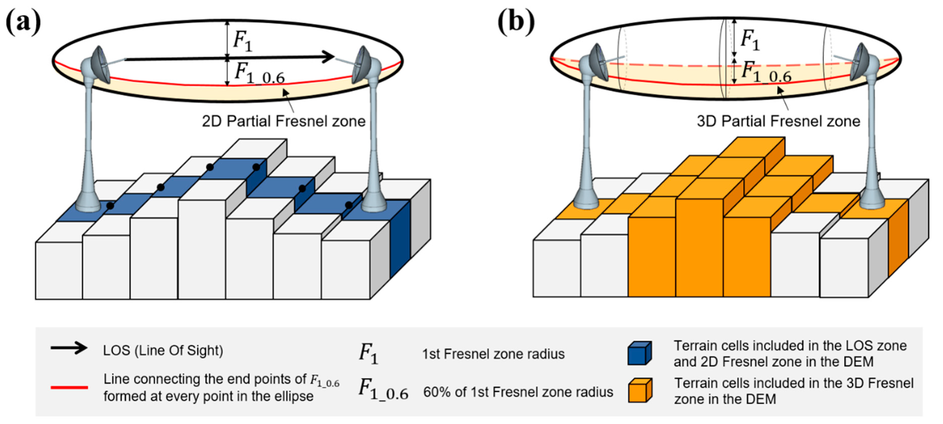
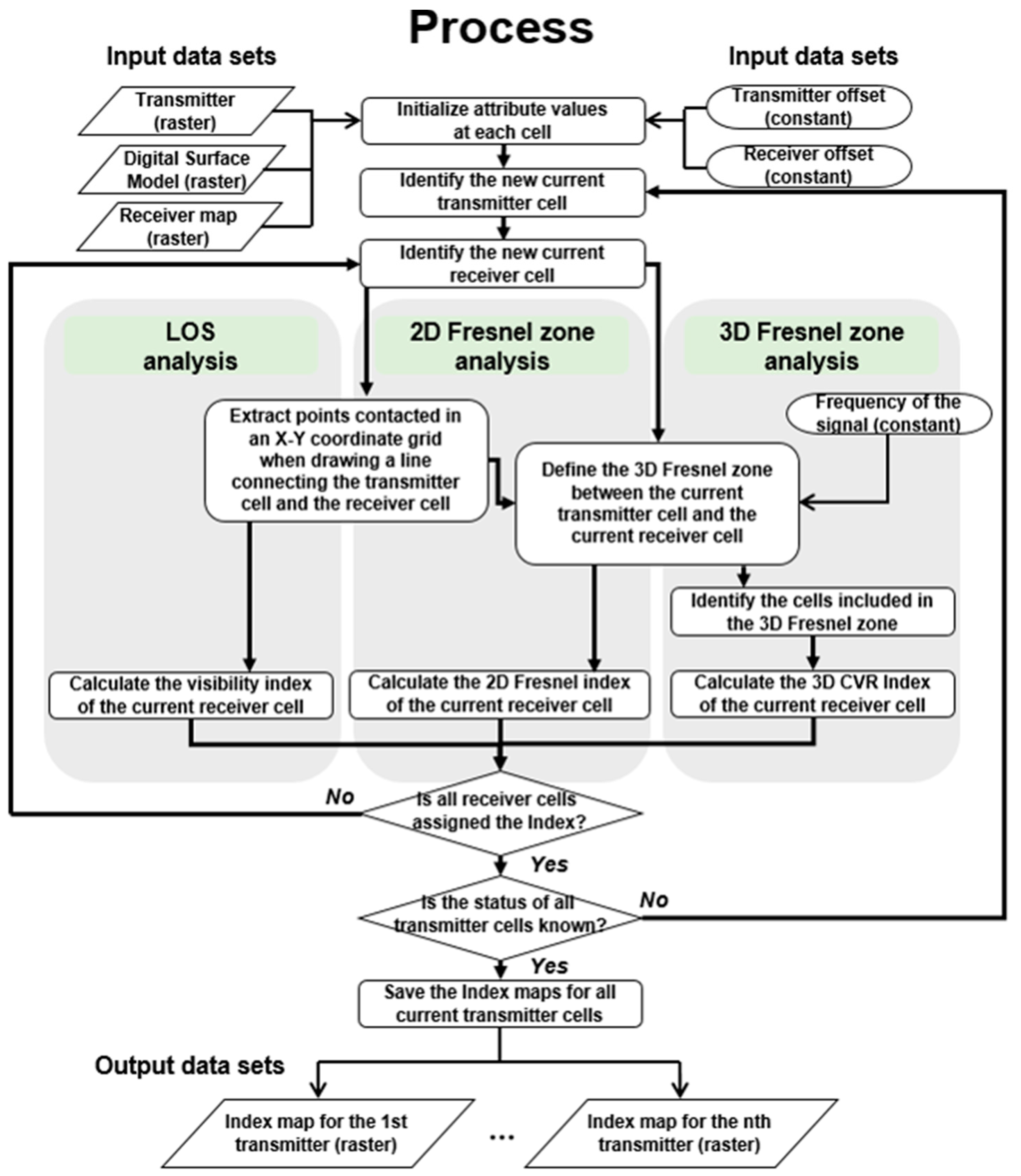
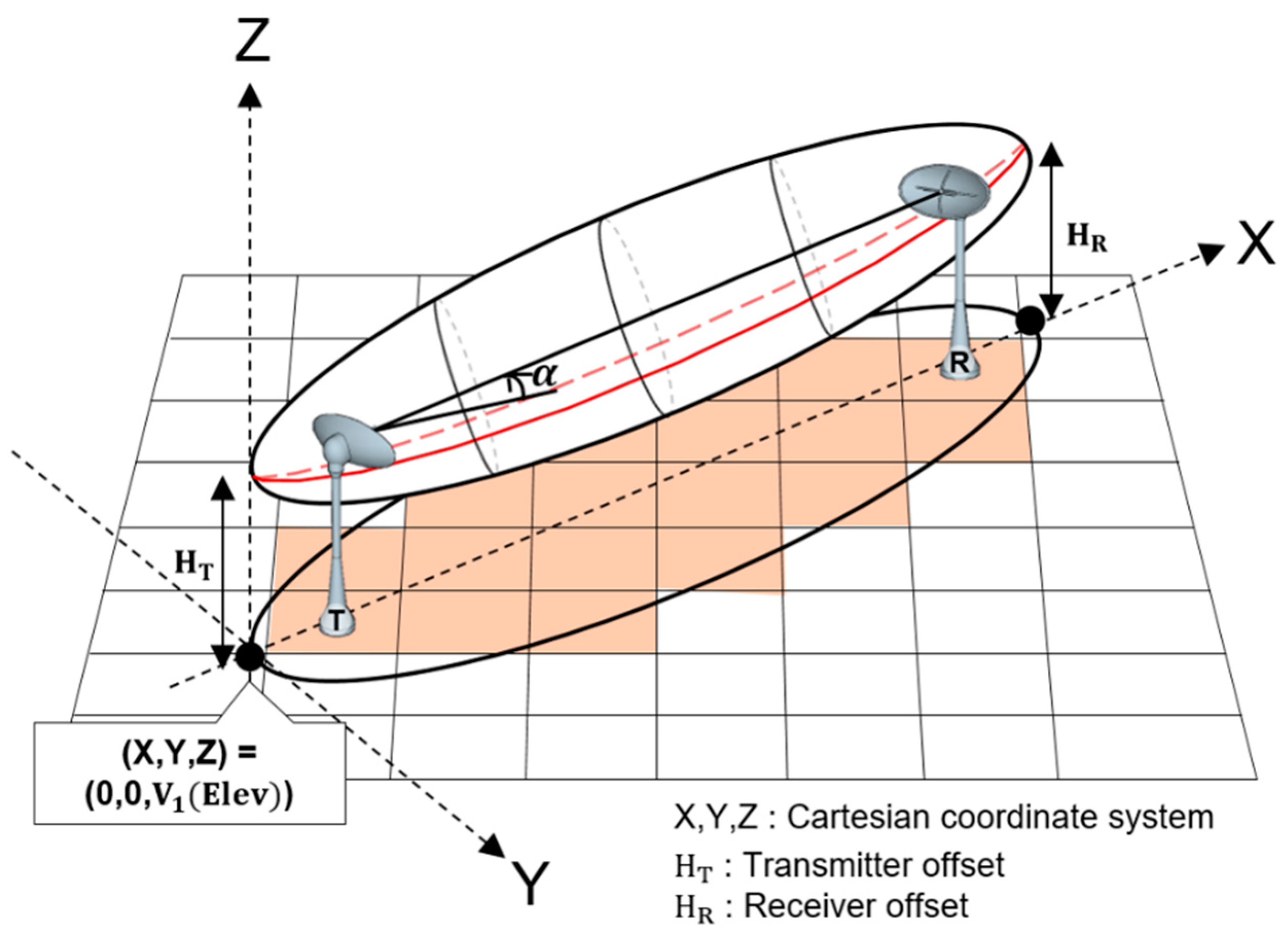
2. Communication Viewsheds Determined by LOS, 2D Fresnel Zone, and 3D Fresnel Zone Analysis

The Fresnel zone is the zone of LOS signal propagation, which has the shape of an ellipsoid of revolution. It is assumed that both the transmitter and the receiver are located at the focal points of the ellipsoid of revolution [47], and that there are innumerable Fresnel zones between the transmitter and the receiver [48]. If the difference between the length of the straight line connecting the transmitter and the receiver and the sum of the lengths of straight lines connecting any point on the ellipsoid of revolution with the transmitter and receiver is $\mathrm{n}·\frac{\mathrm{\lambda }}{2}$, then the ellipsoid of revolution can be defined by the n-th Fresnel zone [47]. If there is an obstacle, such as a geographic feature, tree, or building, then this obstacle generates an echo, which results in an unstable signal level obtained by the receiver [48]. Accordingly, to achieve stable LOS signal propagation, the volume ratio of an obstacle should be 40% or lower, which is included in a partial Fresnel zone between the surface, and is 0.6 times the radius of the Fresnel zone away from the longitudinal section and the lower surface of the first Fresnel zone [52].

Figure 1 presents conceptual diagrams showing the principals for identifying the potential for communication between the transmitter and the receiver through LOS analysis and 2D Fresnel zone analysis and the principals for evaluating communication stability using 3D Fresnel zone analysis. In LOS and 2D Fresnel zone analysis, every cell and point connected on the surface grid along the LOS is extracted, and the terrain altitude of contact points and the LOS altitude or altitude of the upper 2D partial Fresnel zone surface are compared to identify the possibility of communication (Figure 1a). In contrast, 3D Fresnel zone analysis extracts all cells included in the 3D Fresnel zone and compares the terrain altitudes of these cells and those of the upper and lower surfaces of the 3D partial Fresnel zone to calculate communication stability (Figure 1b).

Figure 2 compares the numbers of cells included in 3D Fresnel zones for low-resolution and high-resolution topographic data, respectively. In the low-resolution topographic data, all cells where the LOS contacts the surface grid match those included in the 3D Fresnel zone. However, in the high-resolution topographic data, there is a discrepancy between the cells included in the 3D Fresnel zone and those of the LOS zone; more cells are included in the 3D Fresnel zone. Accordingly, to judge the potential for communication using high-resolution topographic data, a 3D Fresnel zone analysis technique is required that can evaluate communication stability by extracting all cells in 3D Fresnel zones.

Conventional methods using low-resolution topographic data cannot accurately identify vegetation that affects signal propagation, which hinders accurate analysis of communication potential. As unmanned aerial vehicles (UAVs) become more common for conducting topographic surveys, high-resolution topographic data can be obtained more conveniently; thus, vegetation is becoming easier to detect in the data [53,54,55,56]. Therefore, we developed a new 3D Fresnel zone analysis method that can utilize high-resolution DSM data to accurately analyze the possibility of communication by considering the impact of vegetation.

In a 2D Fresnel zone analysis, if the terrain altitude of contact points exceeds the upper surface altitude of the 2D partial Fresnel zone, communication is judged to be impossible; otherwise, communication is considered possible. If the altitude of an obstacle does not exceed the upper surface altitude of the 2D partial Fresnel zone, but it exceeds the lower surface altitude, communication between the transmitter and the receiver is possible but communication stability is low due to the obstacle in the partial Fresnel zone. Accordingly, a new 3D Fresnel index system should be able to quantitatively calculate communication stability by considering cell volumes within the 3D partial Fresnel zone.

3. Principles of LOS, 2D Fresnel Zone, and 3D Fresnel Zone Analysis Methods

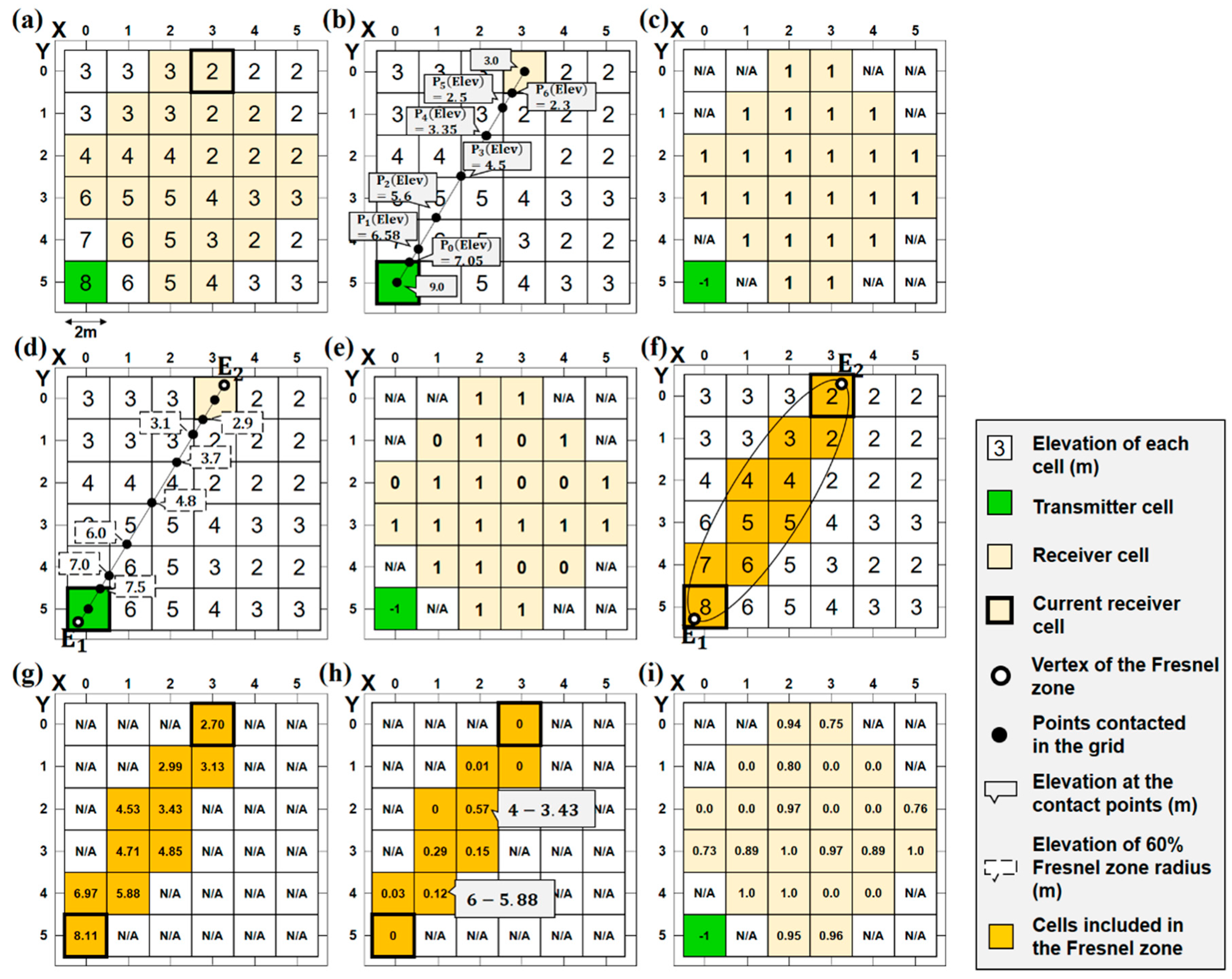
The flow chart in Figure 3 shows the respective processes for LOS analysis, 2D Fresnel zone analysis, and 3D Fresnel zone analysis. Input data for the analysis of the coverage area include a transmitter map showing the location of the transmitter, a receiver map showing the receiving area within the terrain, and a DSM indicating the altitude of the terrain (see Figure 4a). The transmitter map can include all transmitter points within a study area. Other input data include the heights (m) of the transmitter and the receiver, as well as the frequency of the signal (Hz). When the data have been inputted completely, the property values (e.g., index values) of every cell constituting a raster layer are initialized, and the location of the transmitter is identified on the transmitter map. If there are multiple transmitter points, one transmitter is randomly selected and designated as the current transmitter cell. Similarly, one cell is randomly selected among all cells included in the signal receiving area and designated as the current receiver cell. The altitude of the current transmitter cell is changed to the sum of the terrain altitude and the transmitter height, while the altitude of the current receiver cell is changed to the sum of the terrain altitude and the receiver height. For these steps, the xy coordinate grid system is used.

3.1. LOS Analysis

The LOS analysis creates a LOS that connects two cells to judge the possibility of communication between the current transmitter cell and the current receiver cell. A LOS analysis extracts all the points where the LOS contacts the xy coordinate grid (Figure 4b). The slope comparison method is used to compare the altitude of every contact point with the LOS altitude [6]. The terrain slope between the current transmitter cell and the current receiver cell is calculated using the following equations.

$$\mathrm{D}=\sqrt{{\left(\left(\mathrm{T}\left(\mathrm{x}\right)-\mathrm{R}\left(\mathrm{x}\right)\right)\times \mathrm{C}\right)}^2+{\left(\left(\mathrm{T}\left(\mathrm{y}\right)-\mathrm{R}\left(\mathrm{y}\right)\right)\times \mathrm{C}\right)}^2}$$

(1)

$${\mathsf{\theta }}_{\mathrm{T}\to \mathrm{R}}={\tan }^{-1}\frac{\mathrm{H}}{\mathrm{D}}\{\begin{array}{cc}\mathrm{H}=\mathrm{T}\left(\mathrm{Elev}\right)-\mathrm{R}\left(\mathrm{Elev}\right)& \mathrm{if},\mathrm{T}\left(\mathrm{Elev}\right)>\mathrm{R}\left(\mathrm{Elev}\right)\\ \mathrm{H}=\mathrm{R}\left(\mathrm{Elev}\right)-\mathrm{T}\left(\mathrm{Elev}\right)& \mathrm{if},\mathrm{T}\left(\mathrm{Elev}\right)\le \mathrm{R}\left(\mathrm{Elev}\right)\end{array}$$

(2)

In Equations (1) and (2), $\mathrm{D}$ is the distance between the current transmitter cell and the current receiver cell (m), $\mathrm{T}\left(\mathrm{x}\right),\mathrm{T}\left(\mathrm{y}\right),\mathrm{T}\left(\mathrm{Elev}\right)$ indicates the x and y coordinates and the terrain altitude (m) of the current transmitter cell, $\mathrm{R}\left(\mathrm{x}\right),\mathrm{R}\left(\mathrm{y}\right),\mathrm{R}\left(\mathrm{Elev}\right)$ indicates the x and y coordinates and the terrain altitude (m) of the current receiver cell, $\mathrm{C}$ is the size of the raster cell (m), ${\mathsf{\theta }}_{\mathrm{T}\to \mathrm{R}}$ is the terrain slope (degrees) between the current transmitter cell and the current receiver cell, and $\mathrm{H}$ indicates the difference in terrain altitude (m) between the current transmitter and the current receiver cell. In Equations (3) and (4), the terrain slope is calculated between the i-th contact point and the current transmitter cell or the current receiver cell. The terrain slope between every calculated contact point and the current transmitter or receiver cell is compared with the terrain slope between the current transmitter and receiver cell in order to calculate the visibility index in Equation (5) (Figure 4c).

$${\mathrm{P}}_{\mathrm{i}}\left(\mathrm{D}\right)=\{\begin{array}{cc}\sqrt{{\left(\left({\mathrm{P}}_{\mathrm{i}}\left(\mathrm{x}\right)-\mathrm{R}\left(\mathrm{x}\right)\right)\times \mathrm{C}\right)}^2+{\left(\left({\mathrm{P}}_{\mathrm{i}}\left(\mathrm{y}\right)-\mathrm{R}\left(\mathrm{y}\right)\right)\times \mathrm{C}\right)}^2}& \mathrm{if},\mathrm{T}\left(\mathrm{Elev}\right)>\mathrm{R}\left(\mathrm{Elev}\right)\mathrm{i}=0,1,2,\cdots ,\mathrm{n}\\ \sqrt{{\left(\left({\mathrm{P}}_{\mathrm{i}}\left(\mathrm{x}\right)-\mathrm{T}\left(\mathrm{x}\right)\right)\times \mathrm{C}\right)}^2+{\left(\left({\mathrm{P}}_{\mathrm{i}}\left(\mathrm{y}\right)-\mathrm{T}\left(\mathrm{y}\right)\right)\times \mathrm{C}\right)}^2}& \mathrm{if},\mathrm{T}\left(\mathrm{Elev}\right)\le \mathrm{R}\left(\mathrm{Elev}\right)\mathrm{i}=0,1,2,\cdots ,\mathrm{n}\end{array}$$

(3)

$${\mathrm{P}}_{\mathrm{i}}\left(\mathsf{\theta }\right)=\frac{{\mathrm{P}}_{\mathrm{i}}\left(\mathrm{H}\right)}{{\mathrm{P}}_{\mathrm{i}}\left(\mathrm{D}\right)}\{\begin{array}{cc}{\mathrm{P}}_{\mathrm{i}}\left(\mathrm{H}\right)={\mathrm{P}}_{\mathrm{i}}\left(\mathrm{Elev}\right)-\mathrm{R}\left(\mathrm{Elev}\right)& \mathrm{if},\mathrm{T}\left(\mathrm{Elev}\right)>\mathrm{R}\left(\mathrm{Elev}\right)\\ {\mathrm{P}}_{\mathrm{i}}\left(\mathrm{H}\right)={\mathrm{P}}_{\mathrm{i}}\left(\mathrm{Elev}\right)-\mathrm{T}\left(\mathrm{Elev}\right)& \mathrm{if},\mathrm{T}\left(\mathrm{Elev}\right)\le \mathrm{R}\left(\mathrm{Elev}\right)\end{array}$$

(4)

$${\mathrm{CRC}}_{\mathrm{l}}\left(\mathrm{VI}\right)=\{\begin{array}{c}\begin{array}{cc}1& \mathrm{if},{\mathsf{\theta }}_{\mathrm{T}\to \mathrm{R}}>{\mathrm{P}}_{\mathrm{i}}\left(\mathsf{\theta }\right)\mathrm{l}=0,1,2,\cdots ,\mathrm{q}\end{array}\\ \begin{array}{cc}0& \mathrm{if},{\mathsf{\theta }}_{\mathrm{T}\to \mathrm{R}}\le {\mathrm{P}}_{\mathrm{i}}\left(\mathsf{\theta }\right)\mathrm{l}=0,1,2,\cdots ,\mathrm{q}\end{array}\end{array}$$

(5)

In Equations (3)–(5), ${\mathrm{P}}_{\mathrm{i}}\left(\mathrm{D}\right)$ and ${\mathrm{P}}_{\mathrm{i}}\left(\mathsf{\theta }\right)$ are the distance (m) and the terrain slope, respectively, between the i-th contact point and the current transmitter or receiver cell. ${\mathrm{P}}_{\mathrm{i}}\left(\mathrm{x}\right)$, ${\mathrm{P}}_{\mathrm{i}}\left(\mathrm{y}\right),$ and ${\mathrm{P}}_{\mathrm{i}}\left(\mathrm{Elev}\right)$ are the x and y coordinates and terrain altitude (m) of the i-th contact point, respectively. ${\mathrm{P}}_{\mathrm{i}}\left(\mathrm{H}\right)$ is the difference between the terrain altitude of the i-th contact point and the current transmitter or receiver cell (m), $\mathrm{n}$ is the number of contact points, ${\mathrm{CRC}}_{\mathrm{l}}\left(\mathrm{VI}\right)$ is the visibility index of the $\mathrm{l}$-th current receiver cell, and $\mathrm{q}$ indicates the number of receiver cells within the receiver map. The terrain altitude of each contact point is calculated with bilinear interpolation using the terrain altitudes of four adjacent cells. For details concerning bilinear interpolation, refer to [57].

3.2. 2D Fresnel Zone Analysis

Like a LOS analysis, the 2D Fresnel zone analysis extracts every point contacting the xy coordinate grid using the LOS between the current transmitter cell and the current receiver cell (Figure 4d). To compare all the contact points extracted and the altitude of the upper surface of the 2D partial Fresnel zone, the 3D Fresnel zone equation is defined, which is created between the current transmitter cell and the current receiver cell. A Cartesian coordinate system is introduced to define the 3D Fresnel zone equation.

$$\frac{{\mathrm{x}}^2}{{\mathrm{HMa}}_{3\mathrm{D}}{}^2}+\frac{{\mathrm{y}}^2}{{\mathrm{HMi}}_{3\mathrm{D}}{}^2}+\frac{{\mathrm{z}}^2}{{(0.6·{\mathrm{HMi}}_{3\mathrm{D}})}^2}=1$$

(6)

$$\mathrm{SD}=\sqrt{{\mathrm{D}}^2+{\left(\mathrm{T}\left(\mathrm{Elev}\right)-\mathrm{R}\left(\mathrm{Elev}\right)\right)}^2}$$

(7)

$${\mathrm{HMi}}_{3\mathrm{D}}=0.5·\sqrt{\mathrm{\lambda }·\mathrm{SD}}$$

(8)

$${\mathrm{HMa}}_{3\mathrm{D}}=0.5·\sqrt{{\mathrm{SD}}^2+{\mathrm{HMi}}_{3\mathrm{D}}{}^2}$$

(9)

Equation (6) is the 3D Fresnel zone, where the radius on the z axis is 0.6 times half the minor axis. In Equations (6)–(9), $\mathrm{x}$, $\mathrm{y},$ and $\mathrm{z}$ indicate the x, y, and z axes of the Cartesian coordinate system, respectively. ${\mathrm{HMa}}_{3\mathrm{D}}$ is half the major axis of the 3D ellipsoid of revolution (m) and ${\mathrm{HMi}}_{3\mathrm{D}}$ is half the minor axis of the 3D ellipsoid of revolution (m). The length of the minor axis of the 3D ellipsoid of revolution is obtained using the equation calculating the radius of a Fresnel zone [48]. $\mathrm{SD}$ indicates the 2.5D distance (m) between the current transmitter cell and the current receiver cell, and $\mathrm{\lambda }$ is the wavelength of the signal (m). If the current transmitter cell and the current receiver cell do not have the same terrain altitude, an $\mathsf{\alpha }$ revolution occurs in the y axis direction and the definition of the Fresnel zone in Equation (6) is replaced by Equation (10). In Equation (10), $\mathsf{\alpha }$ indicates the counterclockwise revolution (radian) observed from the positive y axis to the origin.

$$\frac{{\left(\mathrm{x}\cos \mathsf{\alpha }-\mathrm{z}\sin \mathsf{\alpha }\right)}^2}{{\mathrm{HMa}}_{3\mathrm{D}}{}^2}+\frac{{\mathrm{y}}^2}{{\mathrm{HMi}}_{3\mathrm{D}}{}^2}+\frac{{\left(\mathrm{x}\sin \mathsf{\alpha }+\mathrm{z}\cos \mathsf{\alpha }\right)}^2}{{(0.6·{\mathrm{HMi}}_{3\mathrm{D}})}^2}=1$$

(10)

The x and y coordinates and terrain altitudes of two end points (${\mathrm{E}}_1,{\mathrm{E}}_2)$ of the major axis of the 3D ellipsoid of revolution on the xy coordinate grid system are then calculated. The x coordinates (${\mathrm{E}}_1\left(\mathrm{x}\right)$, ${\mathrm{E}}_2\left(\mathrm{x}\right)$) and y coordinates (${\mathrm{E}}_1\left(\mathrm{y}\right)$, ${\mathrm{E}}_2\left(\mathrm{y}\right)$) of the two end points are calculated using half the value of the major axis and half that of the minor axis of the 3D ellipsoid of revolution, the planar angles (radians) between the current transmitter cell, and the current receiver cell on the xy coordinate grid. The terrain altitudes between the two end points (${\mathrm{E}}_1\left(\mathrm{Elev}\right)$, ${\mathrm{E}}_2\left(\mathrm{Elev}\right)$) are calculated with linear interpolation using the terrain altitudes between the current transmitter cell and the current receiver cell. To set the x and y coordinates of ${\mathrm{E}}_1$ as (0,0) in the Cartesian coordinate system, the Fresnel zone defined by Equation (10) is moved by ${\mathrm{HMa}}_{3\mathrm{D}}\times \cos \mathsf{\alpha }$ parallel to the x axis and $-{\mathrm{HMa}}_{3\mathrm{D}}\times \sin \mathsf{\alpha }+{\mathrm{E}}_1\left(\mathrm{Elev}\right)$ parallel to the z axis (Figure 5).

The 2D Fresnel index for the current receiver cell is calculated according to the following three stages:

• The distance between ${\mathrm{E}}_1$ and every contact point is calculated. In Equation (11), ${\mathrm{P}}_{\mathrm{i}}\left(\mathrm{D}\right)$ is the distance (m) between ${\mathrm{E}}_1$ and the i-th contact point.

  $${\mathrm{P}}_{\mathrm{i}}\left(\mathrm{D}\right)=\sqrt{({\left({\mathrm{E}}_1\left(\mathrm{x}\right)-{\mathrm{P}}_{\mathrm{i}}\left(\mathrm{x}\right)\right)}^2\times \mathrm{C}+({\left({\mathrm{E}}_1\left(\mathrm{y}\right)-{\mathrm{P}}_{\mathrm{i}}\left(\mathrm{y}\right)\right)}^2\times \mathrm{C}}\mathrm{i}=0,1,2,\cdots ,\mathrm{n}$$

  (11)
• The upper surface altitude of the 2D partial Fresnel zone at the i-th contact point is calculated by setting ${\mathrm{P}}_{\mathrm{i}}\left(\mathrm{D}\right)$ as the x coordinate and 0 as the y coordinate of the 3D Fresnel zone equation.
• The terrain altitude of every contact point is compared with the upper surface altitude of the 2D partial Fresnel zone to obtain the 2D Fresnel index of the current receiver cell. In Equation (12), ${\mathrm{CRC}}_{\mathrm{l}}\left(2\mathrm{DFI}\right)$ is the 2D Fresnel zone index of the current receiver cell, ${\mathrm{P}}_{\mathrm{i}}\left(\mathrm{UElev}\right)$ is the upper surface altitude of the 2D partial Fresnel zone at the i-th contact point, and ${\mathrm{P}}_{\mathrm{i}}\left(\mathrm{Elev}\right)$ is the terrain altitude of the i-th contact point (m).

  $${\mathrm{CRC}}_{\mathrm{l}}\left(2\mathrm{DFI}\right)=\{\begin{array}{c}\begin{array}{cc}1& \mathrm{if},{\mathrm{P}}_{\mathrm{i}}\left(\mathrm{UElev}\right)>{\mathrm{P}}_{\mathrm{i}}\left(\mathrm{Elev}\right)\mathrm{l}=0,1,2,\cdots ,\mathrm{q}\end{array}\\ \begin{array}{cc}0& \mathrm{if},{\mathrm{P}}_{\mathrm{i}}\left(\mathrm{UElev}\right)\le {\mathrm{P}}_{\mathrm{i}}\left(\mathrm{Elev}\right)\mathrm{l}=0,1,2,\cdots ,\mathrm{q}\end{array}\end{array}$$

  (12)

3.3. 3D Fresnel Zone Analysis

Unlike LOS analysis and 2D Fresnel zone analysis, 3D Fresnel zone analysis extracts every cell that is included in the 2D Fresnel zone and projected on the xy plane, using the 3D Fresnel zone created between the current transmitter cell and the current receiver cell (Figure 4f).

$$\frac{{\left(\mathrm{x}\cos \mathsf{\alpha }-\mathrm{z}\sin \mathsf{\alpha }\right)}^2}{{\mathrm{HMa}}_{3\mathrm{D}}{}^2}+\frac{{\mathrm{y}}^2}{{\mathrm{HMi}}_{3\mathrm{D}}{}^2}+\frac{{\left(\mathrm{x}\sin \mathsf{\alpha }+\mathrm{z}\cos \mathsf{\alpha }\right)}^2}{{({\mathrm{HMi}}_{3\mathrm{D}})}^2}=1$$

(13)

$$\frac{{\mathrm{x}}^2}{{\mathrm{HMa}}_{2\mathrm{D}}{}^2}+\frac{{\mathrm{y}}^2}{{\mathrm{HMi}}_{2\mathrm{D}}{}^2}=1$$

(14)

$${\mathrm{HMi}}_{2\mathrm{D}}=0.5·\sqrt{\mathrm{\lambda }·\mathrm{D}}$$

(15)

$${\mathrm{HMa}}_{2\mathrm{D}}=0.5·\sqrt{{\mathrm{D}}^2+{\mathrm{HMi}}_{2\mathrm{D}}{}^2}$$

(16)

Equation (13) is for a 3D Fresnel zone, while Equation (14) is for a 2D Fresnel zone, obtained from the 3D Fresnel zone projected on the xy plane of the Cartesian coordinate system. In Equation (14), ${\mathrm{HMa}}_{2\mathrm{D}}$ is half the major axis of the 2D Fresnel zone (m) and ${\mathrm{HMi}}_{3\mathrm{D}}$ is half the minor axis of the 2D Fresnel zone (m). Likewise, in Equation (13), in order to set the x and y coordinates of ${\mathrm{E}}_1$ as (0,0) in the Cartesian coordinate system, the 3D Fresnel zone defined by Equation (13) is moved by ${\mathrm{HMa}}_{3\mathrm{D}}\times \cos \mathsf{\alpha }$ parallel to the x axis and $-{\mathrm{HMa}}_{3\mathrm{D}}\times \sin \mathsf{\alpha }+{\mathrm{E}}_1\left(\mathrm{Elev}\right)$ parallel to the z axis.

The 3D Fresnel index for the current receiver cell is calculated according to the following three stages.

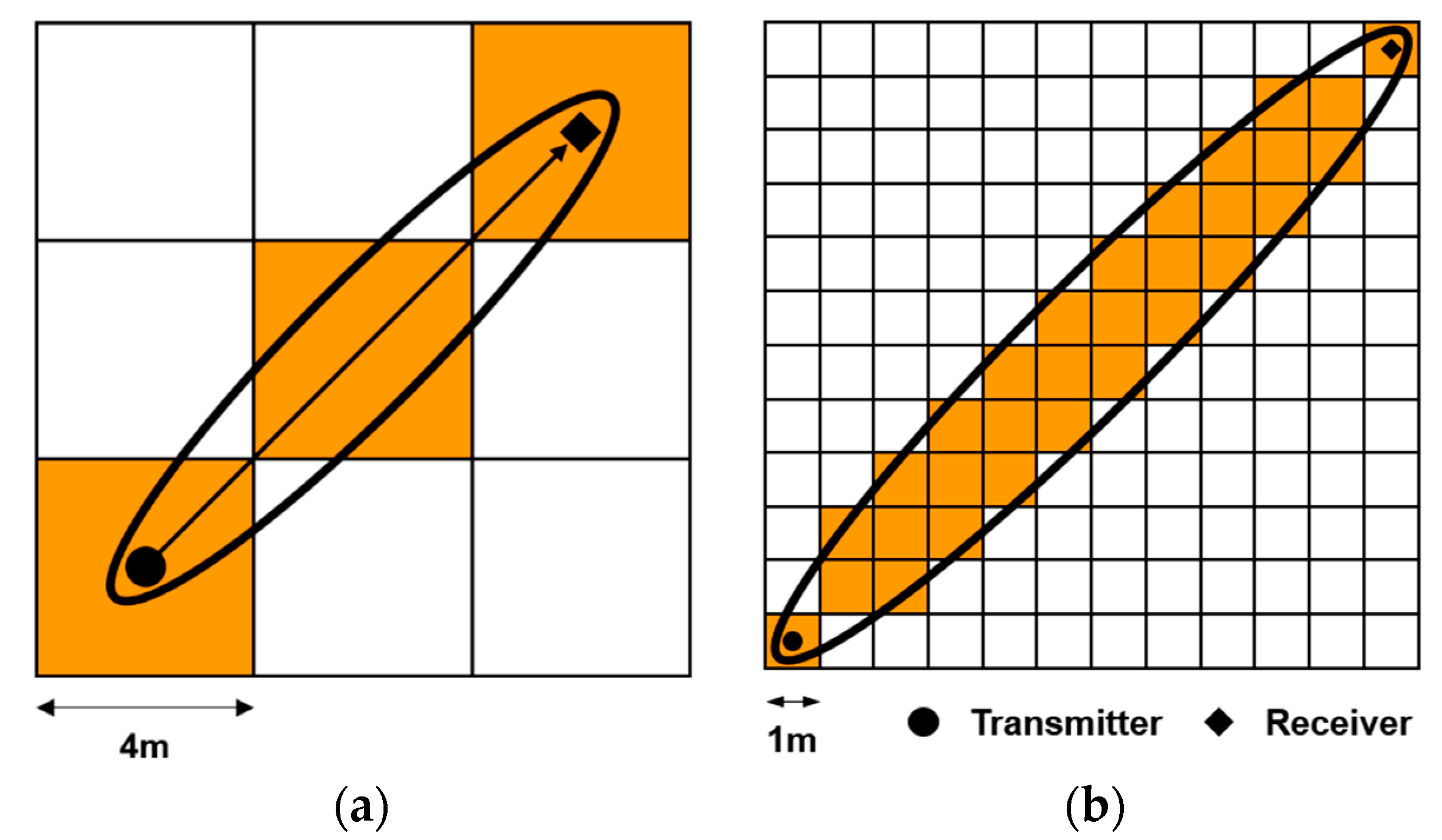
• To extract all cells included in the 3D Fresnel zone, the x and y coordinates of all raster cells in the xy coordinate system are converted into those of the Cartesian coordinate system, which has a straight line connecting ${\mathrm{E}}_1$ and ${\mathrm{E}}_2$ as the x axis. The converted x and y coordinates are inputted into Equation (14) to determine whether a cell is present in the 3D Fresnel zone (Figure 5).
• After extracting only those cells included in the 3D Fresnel zone, the x and y coordinates of the cells are inputted into the 3D partial Fresnel zone and the 3D Fresnel zone equations in order to extract the upper and lower surface altitudes of the 3D partial Fresnel zone at a given cell point (Figure 4g).
• The 3D Fresnel index is calculated by comparing the terrain altitude (m) of the i-th cell included in the 3D Fresnel zone and the upper and lower surface altitudes (m) of the 3D partial Fresnel zone (Figure 4h,i). The 3D Fresnel index is a real number between 0 and 1.

  $${\mathrm{CRC}}_{\mathrm{l}}\left(3\mathrm{DFI}\right)=\{\begin{array}{cc}0& \mathrm{if},{\mathrm{C}}_{\mathrm{i}}\left(\mathrm{Elev}\right)\ge {\mathrm{C}}_{\mathrm{i}}\left(\mathrm{UElev}\right)\mathrm{i}=0,1,2,\cdots ,\mathrm{n}\\ 1-\frac{{{\displaystyle \sum }}_{\mathrm{j}=0}^{\mathrm{m}}{\mathrm{C}}_{\mathrm{j}}\left(\mathrm{V}\right)}{{\mathrm{V}}_{\mathrm{P}}}& \mathrm{if},{\mathrm{C}}_{\mathrm{j}}\left(\mathrm{LElev}\right)<{\mathrm{C}}_{\mathrm{j}}\left(\mathrm{Elev}\right)<{\mathrm{C}}_{\mathrm{j}}\left(\mathrm{UElev}\right)\mathrm{j}=0,1,2,\cdots ,\mathrm{m}\\ 1& \mathrm{if},{\mathrm{C}}_{\mathrm{k}}\left(\mathrm{LElev}\right)\ge {\mathrm{C}}_{\mathrm{k}}\left(\mathrm{Elev}\right)\mathrm{k}=0,1,2,\cdots ,\mathrm{p}\end{array}$$

  (17)

  $${\mathrm{C}}_{\mathrm{j}}\left(\mathrm{V}\right)=\mathrm{C}·\mathrm{C}·\left({\mathrm{C}}_{\mathrm{j}}\left(\mathrm{Elev}\right)-{\mathrm{C}}_{\mathrm{j}}\left(\mathrm{UElev}\right)\right)$$

  (18)

  $${\mathrm{V}}_{\mathrm{P}}=\frac{1}{2}·\left(\frac{4}{3}·\mathsf{\pi }·{\mathrm{HMa}}_{3\mathrm{D}}·{\mathrm{HMi}}_{3\mathrm{D}}{}^2-\frac{4}{3}·\mathsf{\pi }·{\mathrm{HMa}}_{3\mathrm{D}}·{(0.6·{\mathrm{HMi}}_{3\mathrm{D}})}^2\right)$$

  (19)

In Equations (17)–(19), ${\mathrm{CRC}}_{\mathrm{l}}\left(3\mathrm{DFI}\right)$ is the 3D Fresnel index, $\mathrm{n}$ is the number of cells in which the terrain altitudes exceed the upper surface altitude of the 3D partial Fresnel zone, $\mathrm{m}$ is the number of cells in which the terrain altitudes lie between the upper and lower surface altitudes of the 3D partial Fresnel zone, and $\mathrm{p}$ is the number of cells in which the terrain altitudes are lower than the lower surface altitude of the 3D Partial Fresnel zone. ${\mathrm{C}}_{\mathrm{i}}\left(\mathrm{Elev}\right)$ is the terrain altitude of the i-th cell (m), ${\mathrm{C}}_{\mathrm{i}}\left(\mathrm{UElev}\right)$ and ${\mathrm{C}}_{\mathrm{i}}\left(\mathrm{LElev}\right)$ are the upper and lower surface altitudes (m) of the 3D Partial Fresnel zone at the i-the cell point, respectively, ${\mathrm{C}}_{\mathrm{j}}\left(\mathrm{V}\right)$ is the volume of the j-th cell (m²), and ${\mathrm{V}}_{\mathrm{P}}$ is the volume of the 3D partial Fresnel zone (m³).

$${\mathrm{CRC}}_{\mathrm{l}}\left(\mathrm{CI}\right)=\{\begin{array}{cc}1& \mathrm{if},{\mathrm{CRC}}_{\mathrm{l}}\left(\mathrm{VI}\right)>0 \mathrm{or} {\mathrm{CRC}}_{\mathrm{l}}\left(2\mathrm{DFI}\right)>0 \mathrm{or} {\mathrm{CRC}}_{\mathrm{l}}\left(3\mathrm{DFI}\right)>0 \\ 0& \mathrm{if},{\mathrm{CRC}}_{\mathrm{l}}\left(\mathrm{VI}\right)=0{\mathrm{or}\mathrm{CRC}}_{\mathrm{l}}\left(2\mathrm{DFI}\right)=0{\mathrm{or}\mathrm{CRC}}_{\mathrm{l}}\left(3\mathrm{DFI}\right)=0\end{array}$$

(20)

$$\mathrm{CR}=\frac{{{\displaystyle \sum }}_{\mathrm{l}=0}^{\mathrm{q}}{\mathrm{CRC}}_{\mathrm{l}}\left(\mathrm{CI}\right)}{\mathrm{q}}$$

(21)

Based on the calculations for the visibility index, 2D Fresnel index, and 3D Fresnel index of the current receiver cell, the coverage index is calculated using Equation (20). In Equation (20), ${\mathrm{CRC}}_{\mathrm{l}}\left(\mathrm{CI}\right)$ is the coverage index of the current receiver cell. After calculating the coverage index for the current receiver cell, the index calculation is repeated by designating any receiver cell in the receiver map as the current receiver cell. When this calculation is completed for all receiver cells of the receiver map, the coverage ratio for the current transmitter cell is calculated using Equation (21). The index for every receiver cell is calculated by designating any transmitter cell in the transmitter map as the current transmitter cell. If the index calculation is completed for every transmitter cell, then index maps with three types of indexes are stored in the receiver cells. According to the three analysis methods, the visibility index map, 2D Fresnel index map, and 3D Fresnel index map are stored, and the number of index maps is equal to that of transmitter cells.

4. Application of LOS, 2D Fresnel Zone, and 3D Fresnel Zone Analysis

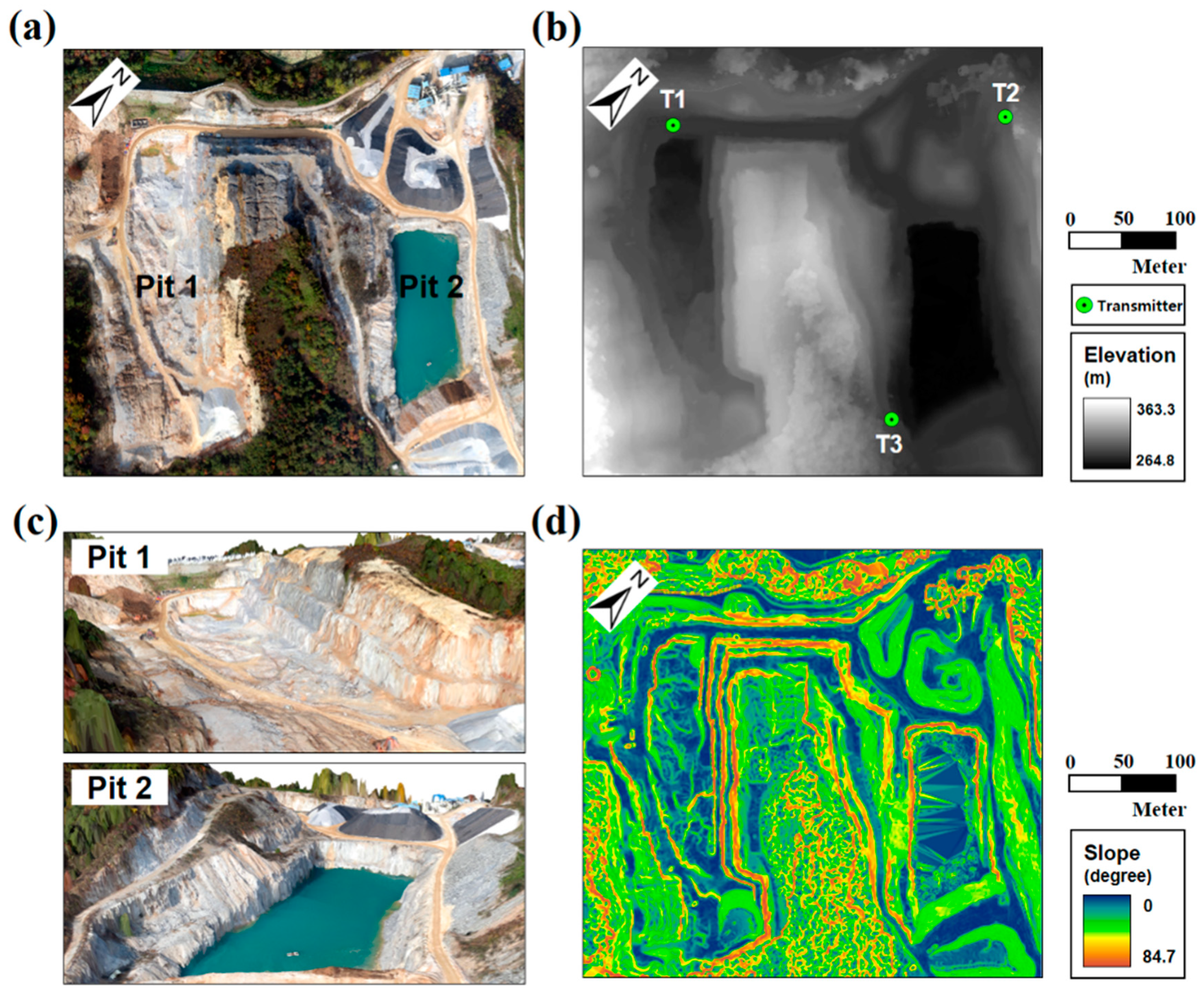
4.1. Study Area and Data

The Seokgyo mine of Daesung MDI, located in Damyang-gun, Chungcheonnam-do, South Korea (37°8′52″ N, 128°20′4″ E), was selected as the study area in order to apply and compare the three methods for determining coverage area. The study area was a small-scale open mine containing two pits which produce high-grade dolomite. The orthoimage in Figure 6a has a resolution of 8 cm per pixel, and was obtained using Postflight Terra 3D, which was incorporated in a SenseFly eBee drone (fixed-wing UAV) that surveyed the topographical features of the study area. We used a resampled DSM with a resolution of 1 m per pixel (columns $\times$ rows: 430 $\times$ 400) to calculate the coverage area of the study area with LOS analysis, 2D Fresnel zone analysis, and 3D Fresnel zone analysis (Figure 6).

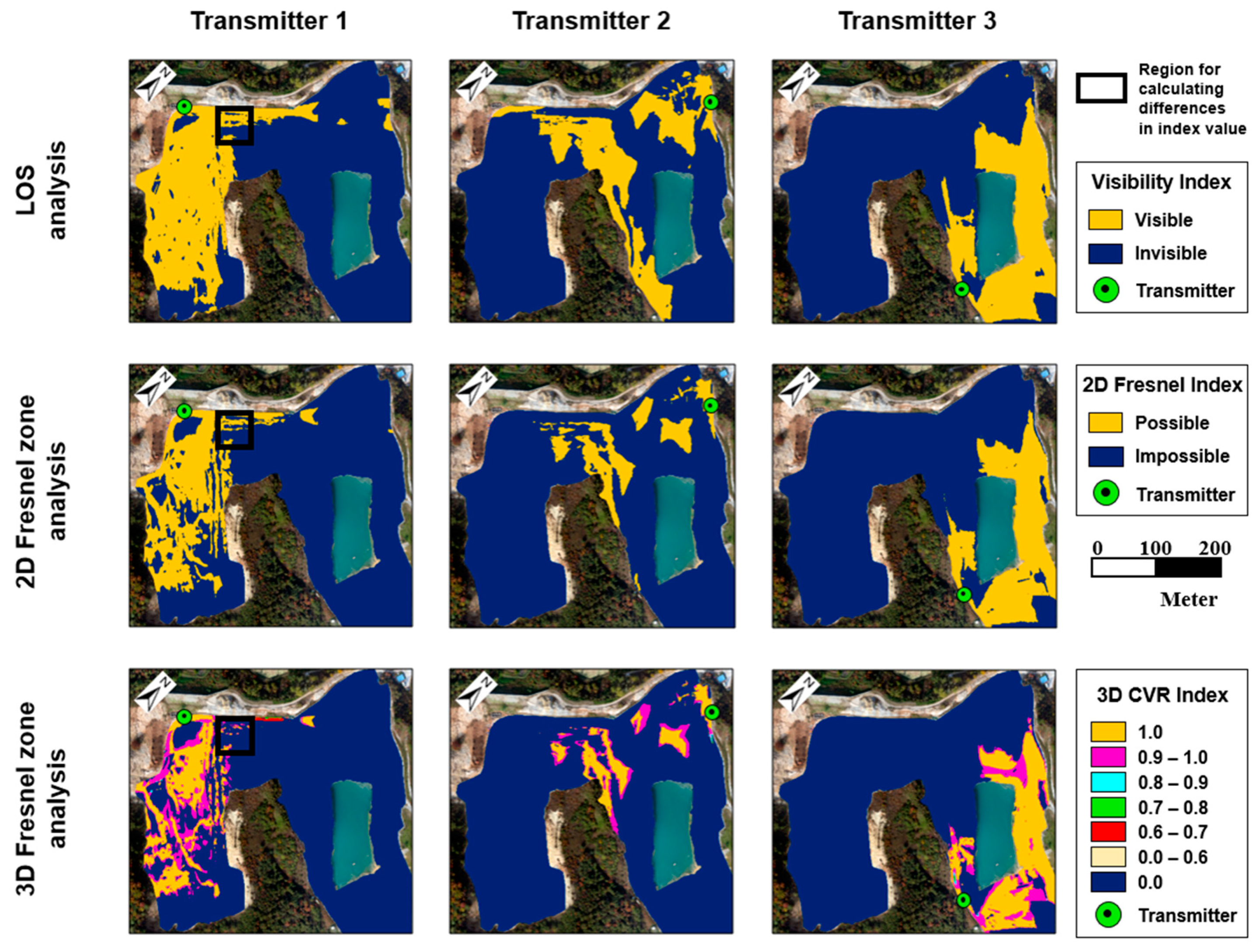
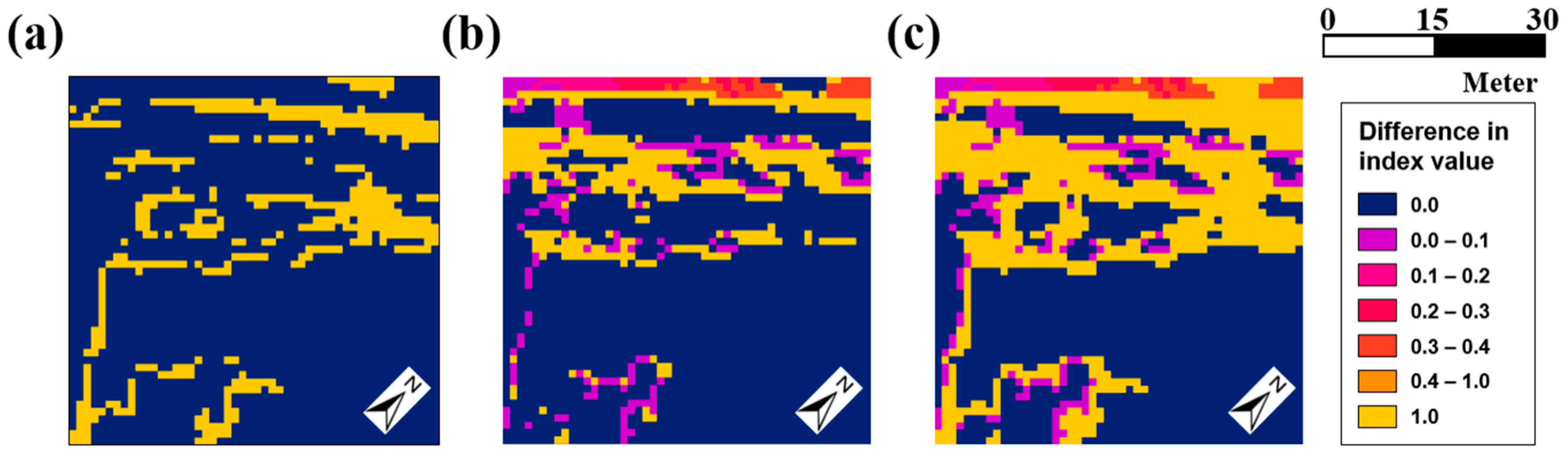
4.2. Communication Viewshed Analysis Using the LOS, 2D Fresnel Zone, and 3D Fresnel Zone Methods

As for the locations of transmitters in the study area, T1 was designated for Pit 1, while T2 and T3 were allocated to Pit 2. The signal reception area was set within a pit (Figure 6b). In addition, the wireless signal frequency was set to 900 MHz (wavelength: 0.333 m) and the heights of the transmitter and receiver were set to 1 m.

Figure 7 shows the visibility index maps, 2D Fresnel index maps, and 3D Fresnel index maps of the signal reception area for three transmitters.

Table 1. Variation of index values and the coverage ratio derived from each method for different transmitter location thresholds.

No. Transmitters	LOS Analysis		2D Fresnel Zone Analysis		3D Fresnel Zone Analysis
	Sum of Visibility Index	Coverage Ratio (%)	Sum of 2D Fresnel Index	Coverage Ratio (%)	Sum of 3D Fresnel Index	Coverage Ratio (%)
T1	32,347	33.96	21,887	22.98	18,091.61	19.19
T2	21,281	22.34	9727	10.21	8474.26	8.93
T3	24,916	26.16	21,445	22.51	20,139.68	21.20
Total	78,544	74.72	53,059	54.83	46,706.33	48.99

presents coverage ratios based on the analysis results in Figure 7. The coverage ratio is the ratio between the sum of index values of all cells and the number of all cells in the signal reception area. In the case of T1, the sum of the visibility indexes of all cells obtained from the LOS analysis was 32,347, while the coverage area constituted 33.96% of the signal reception area. The sum of the 2D Fresnel indexes obtained from the 2D Fresnel zone analysis was 21,887, while the coverage area comprised 22.98% of the total area. The sum of the 3D Fresnel indexes obtained from the 3D Fresnel zone analysis was 18,091.61, and the coverage area covered 19.19% of the open pit mine. When the more advanced technique was used to calculate the coverage area, both the sum of indexes and the coverage ratio tended to decrease; this was because the criterion for calculating the possibility of communication became more conservative.

After using LOS analysis to calculate the coverage areas for transmitters T1, T2, and T3, T1 showed the largest sum of visibility indexes and the highest coverage ratio, while T2 had the lowest values. The 2D Fresnel zone analysis produced the same result; the sum of the 2D Fresnel indexes and the coverage ratio had the largest values at T1 and the lowest values at T2. However, the 3D Fresnel zone analysis showed that the largest values of the sum of the 3D Fresnel indexes and the coverage ratio occurred at T3 and the lowest values occurred at T2. This indicates that, when both vertical and horizontal cells included in the 3D Fresnel zone were considered, communication stability can be more accurately calculated than when only the terrain altitudes of points contacting the LOS are considered in the coverage ratio analysis.

When index maps for T1, T2, and T3 were overlapped to aggregate the index values and calculated coverage ratios, the LOS, 2D Fresnel zone, and 3D Fresnel zone analysis results covered approximately 74.72%, 54.83%, and 48.99% of the signal reception area, respectively.

For some zones of the signal reception area, the three methods were compared in terms of index analysis results for transmitter T1 (Figure 8). The analysis results can be classified into three classes. If the value of any cell was zero, then both methods generated the same communication possibility for the cell. If the value of any cell was 1, one method judged that the communication was possible, but the other method did not. Finally, if the value of any cell was a real number between 0.0 and 1.0, then the respective method judged that communication was possible, while the 3D Fresnel zone analysis produced a 3D Fresnel index of 1.0 or below due to unstable communication. The largest difference occurred between the LOS analysis and the 3D Fresnel zone analysis (Figure 8c). In the remaining two cases, a difference was observed between the index analysis results.

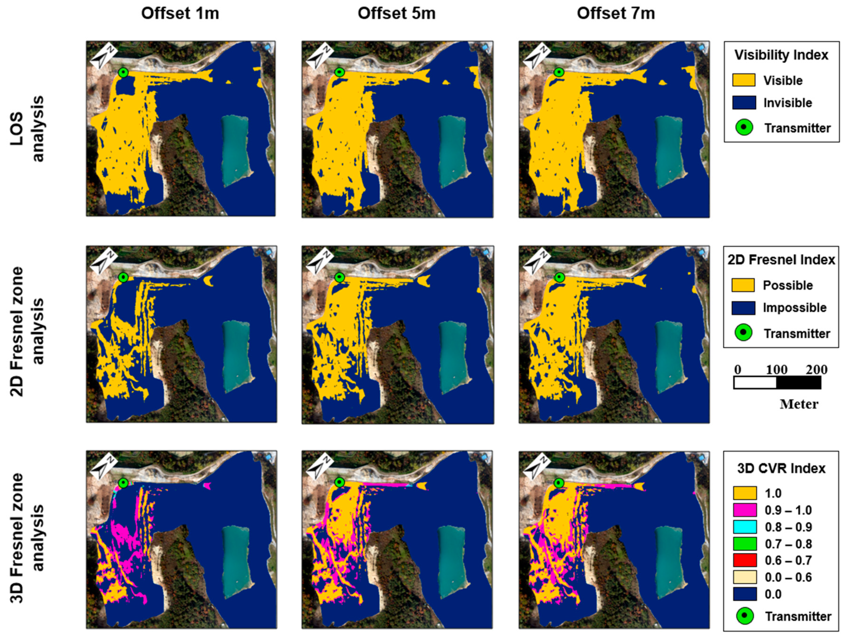
4.3. Communication Viewshed Analysis with Different Transmitter Offset Height Thresholds

The signal frequency and the receiver height were fixed at 900 MHz and 1 m, respectively. The coverage areas were calculated by applying different heights to T1 using the three methods. Figure 9 shows the index maps obtained from each method by applying offset heights of 1 m, 5 m, and 7 m for transmitter T1. When the offset height of the transmitter was set to a lower value, the three methods returned greater differences in communication possibility. The communication stability was calculated as low in most cells in the 3D Fresnel index map. The 3D Fresnel zone analysis showed the highest sensitivity to the transmitter offset height, followed by the 2D Fresnel zone analysis and the LOS analysis. This is because, as transmitter height decreases, the effect of terrain features upon the 3D Fresnel zone between the transmitter and the receiver increases, which results in lower communication stability.

Table 2. Variation of index values and the coverage ratio derived from each method for offset height thresholds of 1 m, 3 m, 5 m, and 7 m.

Offset Height (m)	Viewshed Analysis		2D Fresnel Zone Analysis		3D Fresnel Zone Analysis
	Sum of Visibility Index	Coverage Ratio (%)	Sum of 2D Fresnel Index	Coverage Ratio (%)	Sum of 3D Fresnel Index	Coverage Ratio (%)
1	30,252	31.76	15,779	16.57	12,304.77	13.02
3	32,347	33.96	21,887	22.98	18,091.61	19.19
5	33,486	35.15	24,355	25.57	20,691.59	21.80
7	34,330	36.04	26,157	27.46	22,703.95	23.88

presents the sum of the indexes of all cells analyzed in Figure 9, as well as the coverage ratios for the signal reception area. As the offset height of a transmitter increased, both the sums of the indexes and the coverage ratios calculated by the three methods tended to increase. The coverage ratio obtained from the 3D Fresnel zone analysis increased by approximately 10% when the offset height of the transmitter increased from 1 m to 7 m.

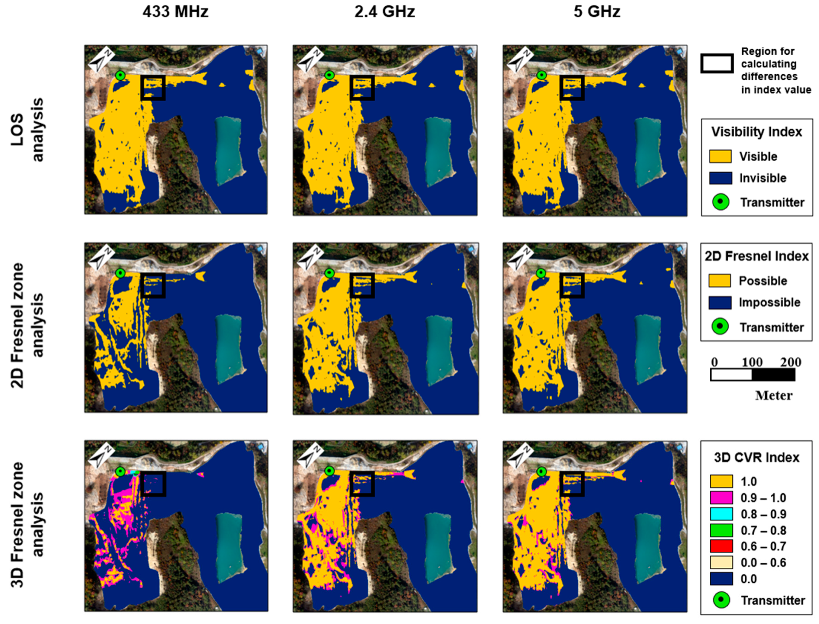
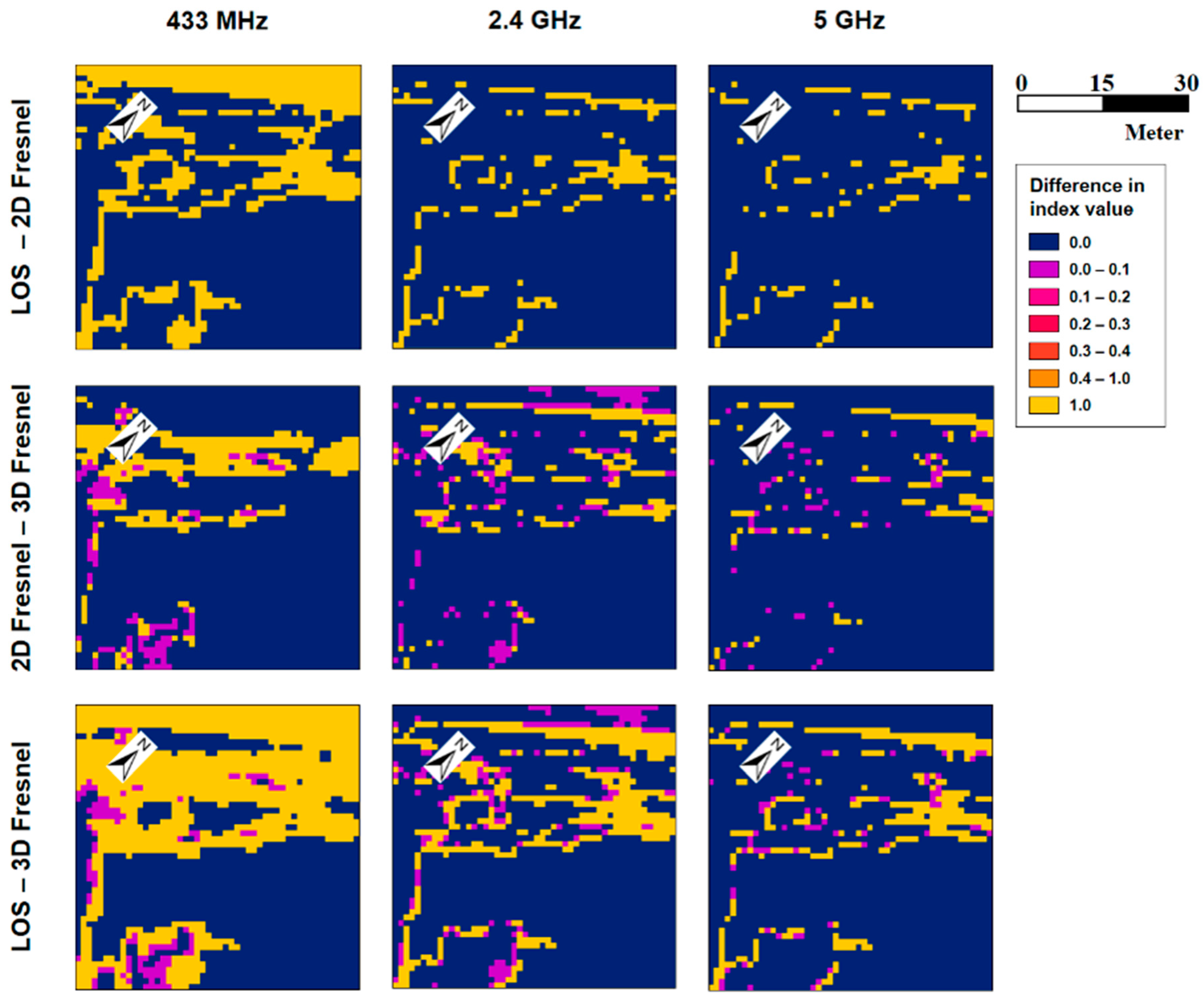
4.4. Communication Viewshed Analysis with Different Frequency Thresholds

The coverage area of transmitter T1 was analyzed by fixing the offset height of the transmitter at 3 m and applying different signal frequencies. The frequency bands used for the analysis were 433 MHz (wavelength: 0.629 m), 2.4 GHz (wavelength: 0.125 m) and 5 GHz (wavelength: 0.06 m) for wireless communication. Figure 10 shows the index maps analyzed using the three methods for T1 at signal frequencies of 433 MHz, 2.4 GHz, and 5 GHz. Because the LOS analysis did not consider any signal frequency, the same visibility index was created in every frequency range. In the 2D Fresnel index map and the 3D Fresnel index map, the lower the signal frequency, the lower the coverage ratio. When the signal frequency was set to a low level, the wavelength increased; thus, both the radius and size of the Fresnel zone increased, which also increased the horizontal cells included in the 3D Fresnel zone. Moreover, the upper surface altitudes of the 2D and 3D partial Fresnel zones were lowered, which made the criterion for communication potential more conservative. On the other hand, when the signal frequency was set to a high level, the wavelength decreased; thus, both the radius and the size of the Fresnel zone decreased, which also decreased the horizontal cells included in the 3D Fresnel zone. In other words, when a higher frequency was set, the criterion for communication potential became more relaxed.

Figure 11 calculates the differences between the visibility index, the 2D Fresnel index, and the 3D Fresnel index of cells in selected zones on the index maps, which were analyzed according to different frequency thresholds. For each frequency threshold, the greatest difference was observed between the visibility index and the 3D Fresnel index. Considering all cells in the study area, the index difference was the highest at the frequency threshold of 433 MHz (see Figure 12). When the signal frequency was set to a higher value, the index difference of the cells gradually decreased. This was because the size of the Fresnel zone became smaller at higher frequencies and the LOS analysis, 2D Fresnel zone analysis, and 3D Fresnel zone analysis exhibited increasingly criteria for communication potential.

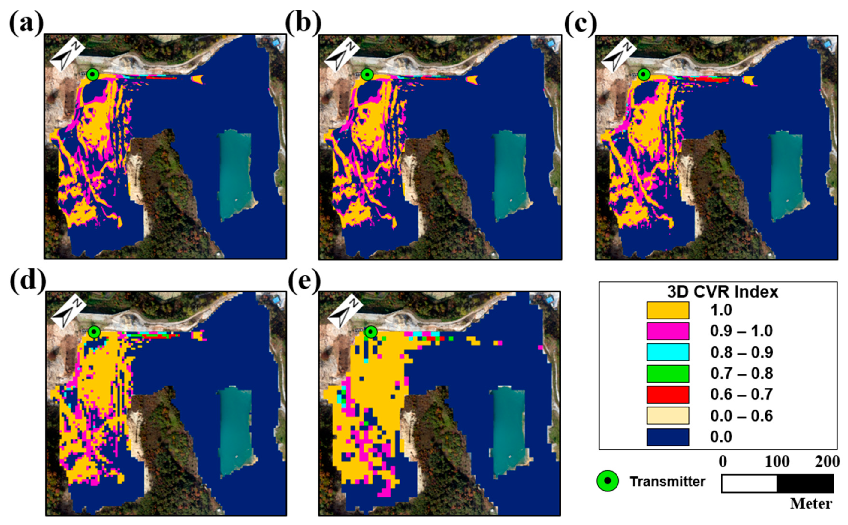
4.5. Communication Viewshed Analysis with Different DSM Resolutions

The communication stability for transmitter T1 was identified using 3D Fresnel zone analysis. When the offset height of the transmitter was fixed at 3 m, the offset height of the receiver was fixed at 1 m and the signal frequency was fixed at 900 MHz, however, different DSM resolutions were applied. The orthoimage of the study area, which was obtained using an UAV, was resampled to create a DSM with resolutions of 0.25 m, 0.5 m, 2 m, 4 m, and 8 m. High-resolution DSMs with pixel sizes of 0.25 m, 0.5 m, 1 m, and 2 m were used to calculate communication stability; each of the results of the 3D Fresnel index map analysis were consistent. On the other hand, the 3D Fresnel index maps that used DSMs with low resolutions of 4 m and 8 m produced inaccurate results. Accordingly, if communication stability is calculated using 3D Fresnel zone analysis, then high-resolution topographical data will produce more accurate results (see Figure 13).

5. Discussion

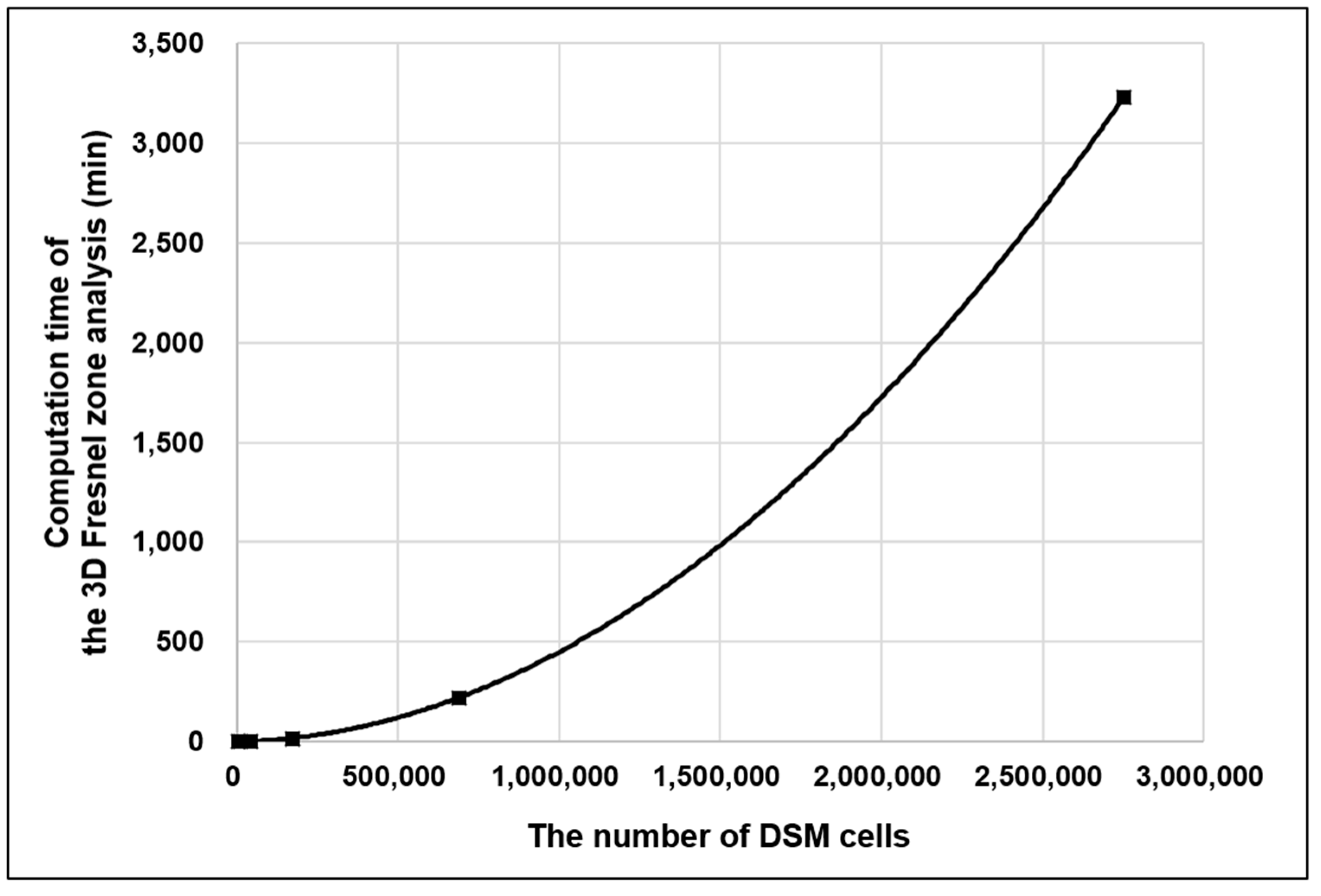
5.1. Comparison of the Computation Time for Each Method

Table 3. Comparison of the computation time for each method at different DSM resolutions.

DSM Resolution (m)	DSM Info.			Computation Time (min)
	Columns	Rows	Number of Cells	LOS Analysis	2D Fresnel Zone Analysis	3D Fresnel Zone Analysis
8	54	50	2700	0.00	0.00	0.02
4	108	100	10,800	0.00	0.00	0.08
2	215	200	43,000	0.03	0.08	1.03
1	430	400	172,000	0.45	1.25	15.73
0.5	860	800	688,000	2.32	6.25	221.75
0.25	1720	1600	2,752,000	18.33	49.22	3230.12

compares DSM information according to different resolutions with the computation time required for different DSM resolutions. The computational specifications used for the comparison of computation time included an Intel(R) Core(TM) i7-2600 CPU (3.40 GHz) and 4 GB RAM running Windows 7. For a DSM resolution of 0.25 m, the computation time of the 3D Fresnel zone analysis was approximately 3230 min, which was approximately 176 times and 66 times longer than the computation time for the LOS analysis and the 2D Fresnel zone analysis, respectively. For a DSM resolution of 2 m, the computation time for the 3D Fresnel zone analysis was approximately 1 min, which was 34 times and 13 times longer than those for the LOS analysis and the 2D Fresnel zone analysis, respectively. Even when the resolution was improved from 2 m to 1 m, 0.5 m, and 0.25 m, the ratio of computation time between LOS analysis and 2D Fresnel zone analysis was maintained at approximately 2.7, while the difference in computation time between the LOS analysis and the 3D Fresnel zone analysis increased exponentially.

As the DSM resolution was improved, the computation time for the LOS analysis, the 2D Fresnel analysis, and the 3D Fresnel analysis increased. Notably, the computation time of the 3D Fresnel zone analysis at a DSM resolution of 0.25 m was approximately 3136 times longer than that at a DSM resolution of 2 m. Figure 14 shows a graph of the computation time of the 3D Fresnel zone analysis according to the number of DSM cells. The computational order of the 3D Fresnel zone analysis is estimated to be about O(n²). For this reason, when the high-resolution digital surface models are used for a communication viewshed analysis, it would be difficult to implement the 3D Fresnel zone analysis in real time. However, recent advances in computer performance make the computation time of the 3D Fresnel zone algorithm less of a serious issue. In addition, the combination of new viewshed techniques (i.e., GPU parallel processing) is expected to enhance computational efficiency.

5.2. Limitations of Communication Viewsheds and Future Works

In the field of communications, the stability of radio signal propagation and the signal coverage area are quantitatively estimated using LOS analysis, 2D Fresnel zone analysis, and 3D Fresnel zone analysis for determining the optimal transmitter placement and for designing wireless communication systems on-site [58,59,60]. However, in practice, electromagnetic phenomena such as attenuation of the wireless signal, the diffraction of ultra-high frequency signals, and surface reflection may make it difficult to stabilize signal propagation between the transmitter and the receiver [61,62,63]. For these reasons, it is difficult to generate a theoretical signal coverage area that corresponds with the coverage area obtained in the field. As a result, significant uncertainty may exist regarding the design of wireless communication systems and their respective performance.

Therefore, in order to estimate the exact signal coverage area of a site through LOS analysis, 2D Fresnel zone analysis, and 3D Fresnel zone analysis, it is necessary to have a precise understanding of the various electromagnetic phenomena that occur when radio signals propagate between the transmitter and the receiver. Furthermore, it is imperative to improve existing GIS-based communication viewshed analysis methods for an accurate signal coverage area analysis that accounts for electromagnetic phenomena. In the future, further site investigation and empirical data acquisition are required to validate the 3D Fresnel zone analysis method. In addition, it would be interesting to analyze the effects of electromagnetic phenomena on the stable LOS signal propagation and develop an advanced 3D Fresnel zone analysis method that considers various electromagnetic phenomena.

6. Conclusions

This study compared the performance of LOS analysis, 2D Fresnel zone analysis, and 3D Fresnel zone analysis for extracting communication viewsheds from high-resolution topographic data. The three methods were applied to calculate coverage ratios for the study area under different transmitter offset heights and signal frequencies. As the offset height and signal frequency decreased, the difference between the results of the three methods tended to increase. When the communication potential was calculated according to different DSM resolutions, the 3D Fresnel zone analysis using higher resolution topographical data produced more accurate and reasonable results.

The 3D Fresnel zone analysis method proposed in this study can accurately analyze coverage areas by employing high-resolution topographical data and accounting for vegetation, which greatly influences communication stability. In addition, the proposed method can quantitatively calculate communication stability by considering all horizontal and vertical terrain cells included in the 3D Fresnel zones.

The receiver map, which is necessary input data for 3D Fresnel zone analysis, can be customized by considering land-use maps or risk maps. Moreover, if there are transmitters with different communication roles in an area, different signal reception areas can be defined according to the type of transmitter. A 3D Fresnel zone analysis can be utilized to determine optimal transmitter locations because it quantitatively compares the sum of the 3D Fresnel indexes of all cells in the receiver map with coverage ratios. Because communication stability is calculated by overlapping 3D Fresnel index maps, which are then analyzed for multiple transmitters, it is possible to estimate the optimal number and the best combination of transmitters.

To improve the computational efficiency of 3D Fresnel zone analysis, the following enhancements are required: (1) a solution to the time-consumption problem through the application of the latest viewshed techniques, such as GPU parallel processing [22,23,24,27]; (2) the efficient application of a large high-resolution DSM processing algorithm [29]; (3) the application of a visibility analysis technique which considers vegetation in the DSM [64,65]; and (4) the consideration of the sampling order of cells included in 3D Fresnel zones [66,67,68].

References

1. Lee, J.; Stucky, D. On Appliying Viewshed Analysis for Determining Least-Cost Paths on Digital Elevation Models. Int. J. Geogr. Inf. Sci. 1998, 12, 891–905. [Google Scholar] [CrossRef]
2. ArcGIS by ESRI. Available online: https://www.esri.com/en-us/arcgis/about-arcgis/overview (accessed on 22 June 2018).
3. GRASS GIS by Open Source Geospatial Foundation (OSGeo). Available online: https://grass.osgeo.org/ (accessed on 22 June 2018).
4. IDRISI by Clark Labs. Available online: https://clarklabs.org/terrset/idrisi-gis/ (accessed on 22 June 2018).
5. Fisher, P.F. First Experiments in Viewshed Uncertainty: The Accuracy of the Viewshed Area. Photogramm. Eng. Remote. Sens. 1991, 57, 1321–1327. [Google Scholar]
6. Sorensen, P.A.; Lanter, D.P. Two Algorithms for Determining Partial Visibility and Reducing Data Structure Induced Error in Viewshed Analysis. Photogramm. Eng. Remote. Sens. 1993, 59, 1149–1160. [Google Scholar]
7. Lee, J. Analyses of Visibility Sites on Topographic Surfaces. Int. J. Geogr. Inf. Syst. 1991, 5, 413–429. [Google Scholar] [CrossRef]
8. Floriani, L.D.; Magillo, P. Visibility Algorithms on Triangulated Digital Terrain Models. Int. J. Geogr. Inf. Syst. 1994, 8, 13–41. [Google Scholar] [CrossRef]
9. Coll, N.; Fort, M.; Madern, N.; Sellarès, J.A. Multi-visibility Maps of Triangulated Terrains. Int. J. Geogr. Inf. Sci. 2007, 21, 1115–1134. [Google Scholar] [CrossRef]
10. De Floriani, L.; Magillo, P. Algorithms for Visibility Computation on Terrains: A Survey. Environ. Plan. B Plan. Des. 2003, 30, 709–728. [Google Scholar] [CrossRef]
11. Huss, R.E.; Pumar, M.A. Effect of Database Errors on Intervisibility Estimation. Photogramm. Eng. Remote. Sens. 1997, 63, 415–424. [Google Scholar]
12. Franklin, R.; Ray, C.R. Higher isn’t necessarily better: Visibility algorithms and experiments. In Proceedings of the Advances in GIS research: 6th international symposium on spatial data handling University of Edinburgh, Edinburgh, UK, 5–9 September 2004; Waugh, T.C., Healey, R.G., Eds.; Taylor & Francis: London, UK, 1994; pp. 751–770. [Google Scholar]
13. Fisher, P.F. Stretching the Viewshed. In Proceedings of the 6th International Symposium on Spatial Data Handling, University of Edinburgh, Edinburgh, UK, 5–10 July; Waugh, T.C., Healey, R.G., Eds.; Taylor & Francis: London, UK, 1994; pp. 725–738. [Google Scholar]
14. Lee, J. Digital Analysis of Viewshed Inclusion and Topographic Features on Digital Elevation Models. Photogramm. Eng. Remote. Sens. 1994, 60, 451–456. [Google Scholar]
15. Rana, S. Fast Approximation of Visibility Dominance Using Topographic Features as Targets and the Associated Uncertainty. Photogramm. Eng. Remote. Sens. 2003, 69, 881–888. [Google Scholar] [CrossRef] [Green Version]
16. Wang, J.; Robinson, G.J.; White, K. A Fast Solution to Local Viewshed Computation Using Grid-Based Digital Elevation Models. Photogramm. Eng. Remote. Sens. 1996, 62, 1157–1164. [Google Scholar]
17. Van Kreveld, M. Variations on Sweep Algorithms: Efficient Computation of Extended Viewsheds and Class Intervals. In Proceedings of the 7th international symposium on spatial data handling: Advances in GIS research II (SDH’96), Delft, The Netherlands, 12–16 August 1996; Kraak, M.J., Molenaar, M., Eds.; TU Delft: Delft, The Netherlands, 1996; pp. 15–27. [Google Scholar]
18. Wang, J.; Robinson, G.J.; White, K. Generating Viewsheds without Using Sightlines. Photogramm. Eng. Remote. Sens. 2000, 66, 87–90. [Google Scholar]
19. Wu, H.; Pan, M.; Yao, L.; Luo, B. A partition-based Serial Algorithm for Generating Viewshed on Massive DEMs. Int. J. Geogr. Inf. Sci. 2007, 21, 955–964. [Google Scholar] [CrossRef]
20. Ogburn, D.E. Assessing the Level of Visibility of Cultural Objects in Past Landscapes. J. Archaeol. Sci. 2006, 33, 405–413. [Google Scholar] [CrossRef]
21. Kidner, D.; Rallings, P.; Ware, J. Parallel processing for terrain analysis in GIS: Visibility as a case study. Geoinformatica 1997, 1, 183–207. [Google Scholar] [CrossRef]
22. Xia, Y.; Li, Y.; Shi, X. Parallel Viewshed Analysis on GPU using CUDA. In Proceedings of the 3th International Joint Conference on Computational Science and Optimization, Huangshan, China, 28–31 May 2010; IEEE: New York, NY, USA, 2010; pp. 373–374. [Google Scholar]
23. Chao, F.; Chongjun, Y.; Zhuo, C.; Xiaojing, Y.; Hantao, G. Parallel algorithm for viewshed analysis on a modern GPU. Int. J. Digit. Earth 2011, 4, 471–486. [Google Scholar] [CrossRef]
24. Gao, Y.; Yu, H.; Liu, Y.; Liu, Y.; Liu, M.; Zhao, Y. Optimization for viewshed analysis on GPU. In Proceedings of the 19th International Conference on Geoinformatics, Shanghai, China, 24–26 June 2011; IEEE: New York, NY, USA, 2011; pp. 1–5. [Google Scholar]
25. Zhao, Y.; Padmanabhan, A.; Wang, S. A parallel computing approach to viewshed analysis of large terrain data using graphics processing units. Int. J. Geogr. Inf. Sci. 2013, 27, 363–384. [Google Scholar] [CrossRef]
26. Ferreira, C.R.; Andrade, M.V.A.; Magalhães, S.V.G.; Franklin, W.R.; Pena, G.C. A Parallel Algorithm for Viewshed Computation on Grid Terrains. J. Inf. Data Manag. 2014, 5, 171–180. [Google Scholar]
27. Osterman, A.; Benedičič, L.; Ritoša, P. An IO-efficient Parallel Implementation of an R2 Viewshed Algorithm for Large Terrain Maps on CUDA GPU. Int. J. Geogr. Inf. Sci. 2014, 28, 2304–2327. [Google Scholar] [CrossRef]
28. Nackaerts, K.; Govers, G.; Orshoven, J. Van Accuracy assessment of probabilistic visibilities. Int. J. Geogr. Inf. Sci. 1999, 13, 709–721. [Google Scholar] [CrossRef]
29. Tabik, S.; Zapata, E.L.; Romero, L.F. Simultaneous computation of total viewshed on large high resolution grids. Int. J. Geogr. Inf. Sci. 2013, 27, 804–814. [Google Scholar] [CrossRef]
30. Bao, S.; Xiao, N.; Lai, Z.; Zhang, H.; Kim, C. Optimizing Watchtower Locations for Forest Fire Monitoring Using Location Models. Fire Saf. J. 2015, 71, 100–109. [Google Scholar] [CrossRef]
31. Chmielewski, S.; Lee, D.J.; Tompalski, P.; Chmielewski, J.T.; Wężyk, P. Measuring Visual Pollution by Outdoor Advertisements in an Urban Street Using Intervisibility Analysis and Public Surveys. Int. J. Geogr. Inf. Sci. 2016, 30, 801–818. [Google Scholar] [CrossRef]
32. Germino, M.J.; Reiners, W.A.; Blasko, B.J.; McLeod, D.; Bastian, C.T. Estimating Visual Properties of Rocky Mountain Landscapes Using GIS. Landsc. Urban Plan. 2001, 53, 71–83. [Google Scholar] [CrossRef]
33. Möller, B. Changing Wind-power Landscapes: Regional Assessment of Visual Impact on Land Use and Population in Northern Jutland, Denmark. Appl. Energy 2006, 83, 477–494. [Google Scholar] [CrossRef]
34. Geneletti, D. Impact assessment of proposed ski areas: A GIS Approach Integrating Biological, Physical and Landscape Indicators. Environ. Impact Assess. Rev. 2008, 28, 116–130. [Google Scholar] [CrossRef]
35. Mouflis, G.D.; Gitas, I.Z.; Iliadou, S.; Mitri, G.H. Assessment of the Visual Impact of Marble Quarry Expansion (1984–2000) on the Landscape of Thasos Island, NE Greece. Landsc. Urban Plan. 2008, 86, 92–102. [Google Scholar] [CrossRef]
36. Danese, M.; Nolè, G.; Murgante, B. Geocomputation, Sustainability and Environmental Planning; Identifying Viewshed: New Approaches to Visual Impact Assessment; Springer: Berlin, Germany, 2011; pp. 73–89. ISBN 978-3-642-19732-1. [Google Scholar]
37. Minelli, A.; Marchesini, I.; Taylor, F.E.; De Rosa, P.; Casagrande, L.; Cenci, M. An Open Source GIS Tool to Quantify the Visual Impact of Wind Turbines and Photovoltaic Panels. Environ. Impact Assess. Rev. 2014, 49, 70–78. [Google Scholar] [CrossRef]
38. Wang, X. Visibility Analysis of Wind Turbines Applied to Assessment of Wind Farms’ Electromagnetic Impact. In Proceedings of the 2013 IEEE 3th International Conference on Information Science and Technology (ICIST), Yangzhou, China, 23–25 March 2013; IEEE: New York, NY, USA, 2013; pp. 1277–1280. [Google Scholar]
39. Castro, M.; De Santos-Berbel, C. Spatial Analysis of Geometric Design Consistency and Road Sight Distance. Int. J. Geogr. Inf. Sci. 2015, 29, 2061–2074. [Google Scholar] [CrossRef]
40. Fontani, F. Application of the Fisher’s “Horizon Viewshed” to a proposed power transmission line in Nozzano (Italy). Trans. GIS 2017, 21, 835–843. [Google Scholar] [CrossRef]
41. Aben, J.; Pellikka, P.; Travis, J.M.J. A call for viewshed ecology: Advancing our understanding of the ecology of information through viewshed analysis. Methods Ecol. Evol. 2018, 9, 624–633. [Google Scholar] [CrossRef]
42. Marsh, E.J.; Schreiber, K. Eyes of the empire: A viewshed-based exploration of Wari site-placement decisions in the Sondondo Valley, Peru. J. Archaeol. Sci. Rep. 2015, 4, 54–64. [Google Scholar] [CrossRef] [Green Version]
43. Dodd, H.M. The Validity of Using a Geographic Information System’s Viewshed Function as a Predictor for the Reception of Line-of-Sight Radio Waves The Validity of Using a Geographic Information System’s Viewshed Function as a Predictor for the Reception of Line. Master’s Thesis, Virginia Tech, Blacksburg, VA, USA, August 2001. [Google Scholar]
44. Bostian, C.; Carstensen, L.; Sweeney, D. Using Geographical Information Systems to Predict Coverage in Broadband Wireless Systems. In Proceedings of the 27th International Union of Radio Science, Maastricht, The Netherlands, 17–24 August 2002; pp. 2–5. [Google Scholar]
45. Popelka, S.; Voženílek, V. Landscape visibility analyses and their visualization. ISPRS Arch. 2010, 38, 1–6. [Google Scholar]
46. Miller, M.L. Analysis of Viewshed Accuracy with Variable Resolution LIDAR Digital Surface Models and Photogrammetrically. Master’s Thesis, Virginia Tech, Blacksburg, VA, USA, October 2011. [Google Scholar]
47. Bertoni, H.L. Radio Propagation for Modern Wireless Systems; Goodwin, B., Ed.; Prentice Hall PTR: Upper Saddle River, NJ, USA, 1999; pp. 1–276. ISBN 0-13-026373-7. [Google Scholar]
48. Campbell Scientific, Inc. Line of Sight Obstruction. Available online: https://s.campbellsci.com/documents/us/technical-papers/line-of-sight-obstruction.pdf (accessed on 23 May 2018).
49. GlobalMapper (Ver.19.1) by Blue Marble Geographics. Available online: http://www.bluemarblegeo.com/products/global-mapper.php (accessed on 22 June 2018).
50. Terrain Analysis Package (TAP) by SoftWright. Available online: https://www.softwright.com/ (accessed on 22 June 2018).
51. Cellular Expert Extension by ESRI. Available online: http://www.cellular-expert.com/ (accessed on 22 June 2018).
52. Coleman, D.D.; Westcott, D.A. CWNA: Certified Wireless Network Administrator Official Study Guide: Exam PW0-105, 3rd ed.; Kellum, J., Ed.; Wiley: New York, NY, USA, 2012; pp. 1–768. ISBN 978-1-118-12779-7. [Google Scholar]
53. Lee, S.; Choi, Y. Topographic Survey at Small-scale Open-pit Mines using a Popular Rotary-wing Unmanned Aerial Vehicle (Drone). Tunn. Undergr. Space Technol. 2015, 25, 462–469. [Google Scholar] [CrossRef]
54. Lee, S.; Choi, Y. On-site Demonstration of Topographic Surveying Techniques at Open-pit Mines using a Fixed-wing Unmanned Aerial Vehicle (Drone). Tunn. Undergr. Space Technol. 2015, 25, 527–533. [Google Scholar] [CrossRef] [Green Version]
55. Lee, S.; Choi, Y. Comparison of Topographic Surveying Results using a Fixed-wing and a Popular Rotary-wing Unmanned Aerial Vehicle (Drone). Tunn. Undergr. Space Technol. 2016, 26, 24–31. [Google Scholar] [CrossRef] [Green Version]
56. Lee, S.; Choi, Y. Reviews of unmanned aerial vehicle (Drone) technology trends and its applications in the mining industry. Geosyst. Eng. 2016, 19, 197–204. [Google Scholar] [CrossRef]
57. Chang, K. Introduction to Geographic Information Systems, 8th ed.; McGraw-Hill Education: New York, NY, USA, 2015; pp. 1–445. ISBN 978-9814636216. [Google Scholar]
58. Sherali, H.D.; Pendyala, C.M.; Rappaport, T.S. Optimal location of transmitters for micro-cellular radio communication system design. IEEE J. Sel. Areas Commun. 1996, 14, 662–673. [Google Scholar] [CrossRef]
59. Jaber, M.; Dawy, Z.; Akl, N.; Yaacoub, E. Tutorial on LTE/LTE-A Cellular Network Dimensioning Using Iterative Statistical Analysis. IEEE Commun. Surv. Tutor. 2016, 18, 1355–1383. [Google Scholar] [CrossRef]
60. Puspitasari, N.F.; Al Fatta, H.; Wibowo, F.W. Layout Optimization of Wireless Access Point Placement Using Greedy and Simulated Annealing Algorithms. Network 2016, 2, 1–12. [Google Scholar] [CrossRef]
61. Freeman, R.L. Fundamentals of Telecommunications, 2nd ed.; John Wiley & Sons: Hoboken, NJ, USA, 2005; pp. 1–720. ISBN 9780471720935. [Google Scholar]
62. Parsons, J.D. The Mobile Radio Propagation Channel, 2nd ed.; John Wiley & Sons: Chichester, UK, 2000; pp. 1–401. ISBN 978-0-471-98857-1. [Google Scholar]
63. White, R.F. Engineering Considerations for Microwave Communications Systems; Lenkurt Electric Co., Inc.: San Carlos, CA, USA, 1970; pp. 1–119. [Google Scholar]
64. Llobera, M. Modeling Visibility through Vegetation. Int. J. Geogr. Inf. Sci. 2007, 21, 799–810. [Google Scholar] [CrossRef]
65. Murgoitio, J.J.; Shrestha, R.; Glenn, N.F.; Spaete, L.P. Improved Visibility Calculations with Tree Trunk Obstruction Modeling from Aerial LiDAR. Int. J. Geogr. Inf. Sci. 2013, 27, 1865–1883. [Google Scholar] [CrossRef]
66. Yu, T.; Xiong, L.; Cao, M.; Wang, Z.; Zhang, Y.; Tang, G. A New Algorithm Based on Region Partitioning for Filtering Candidate Viewpoints of a Multiple Viewshed. Int. J. Geogr. Inf. Sci. 2016, 30, 2171–2187. [Google Scholar] [CrossRef]
67. Shi, X.; Xue, B. Deriving a Minimum Set of Viewpoints for Maximum Coverage over any Given Digital Elevation Model Data. Int. J. Digit. Earth 2016, 9, 1153–1167. [Google Scholar] [CrossRef]
68. Bartie, P.; Mackaness, W. Improving the Sampling Strategy for Point-to-point Line-of-sight modelling in Urban Environments. Int. J. Geogr. Inf. Sci. 2017, 31, 805–824. [Google Scholar] [CrossRef]
Figure 1. Conceptual view showing the process for estimating signal coverage using (a) LOS analysis and 2D Fresnel zone analysis; and (b) 3D Fresnel zone analysis.
Ijgi 07 00322 g001
Figure 2. Comparison of the cells included in the 1st Fresnel zone when using a (a) low-resolution DSM and (b) high-resolution DSM.
Ijgi 07 00322 g002
Figure 3. Flow chart showing procedures for communication viewshed analysis using LOS analysis, 2D Fresnel zone analysis, and 3D Fresnel zone analysis.
Ijgi 07 00322 g003
Figure 4. An example of calculating index maps for all cells when the transmitter offset and the receiver offset is 1 m and the wavelength of the signal is also 1 m. (a) Identifying the current transmitter cell and the current receiver cell; (b) extracting all contact points on the LOS connecting the current transmitter cell and receiver cell; (c) visibility index map; (d) extracting all contact points on the LOS connecting two vertexes of the Fresnel zone; (e) 2D Fresnel index map; (f) extracting all cells included in the 3D Fresnel zone; (g) elevation raster for the lower surface of the 3D Fresnel zone; (h) differences of elevation between extracted cells and the lower surface of the 3D Fresnel zone; and (i) 3D CVR index map.
Ijgi 07 00322 g004
Figure 5. Conceptual view showing the procedure for transforming the coordinate system from the xy coordinate grid to the modified Cartesian coordinate system.
Ijgi 07 00322 g005
Figure 6. Real-world data sets used to test the algorithm. (a) Orthographic image of the open-pit mine obtained using the SenseFly eBee drone. Reference grid is in m and the coordinate system of the image is local transverse Mercator; (b) DSM of the study area (resolution = 1 m); (c) 3-dimensional views of the study area; and (d) distribution of the slope (degrees).
Ijgi 07 00322 g006
Figure 7. Index maps generated by LOS analysis, 2D Fresnel zone analysis, and 3D Fresnel zone analysis for transmitter 1, transmitter 2, and transmitter 3 in the study area.
Ijgi 07 00322 g007
Figure 8. Differences in index maps obtained by (a) the LOS analysis and the 2D Fresnel zone analysis, (b) the 2D Fresnel zone analysis and the 3D Fresnel zone analysis, and (c) the LOS analysis and the 3D Fresnel zone analysis for transmitter 1.
Ijgi 07 00322 g008
Figure 9. Index maps produced by each method for transmitter 1 for a frequency threshold of 900 MHz and transmitter offset heights of 1 m, 5 m, and 7 m.
Ijgi 07 00322 g009
Figure 10. Index maps for transmitter 1 generated by each method for a transmitter offset height of 3 m and frequency thresholds of 433 MHz, 2.4 GHz, and 5 GHz.
Ijgi 07 00322 g010
Figure 11. Differences between visibility index maps, 2D Fresnel index maps, and 3D Fresnel index maps for transmitter 1 at a frequency threshold of 433 MHz, 2.4 GHz, and 5 GHz.
Ijgi 07 00322 g011
Figure 12. Differences in index value of all raster cells in the study area at different frequency thresholds.
Ijgi 07 00322 g012
Figure 13. 3D Fresnel index maps for transmitter 1 with DSM resolutions of (a) 25 cm, (b) 50 cm, (c) 2 m, (d) 4 m, and (e) 8 m.
Ijgi 07 00322 g013
Figure 14. The computation time needed for the 3D Fresnel zone analysis according to the number of DSM cells.
Ijgi 07 00322 g014