Spatially Explicit Age Segregation Index and Self-Rated Health of Older Adults in US Cities


Department of Geography, University of Florida, P.O. Box 117315, 3141 Turlington Hall, Gainesville, FL 32611, USA
*
Author to whom correspondence should be addressed.
ISPRS Int. J. Geo-Inf. 2018, 7(9), 351; https://0-doi-org.brum.beds.ac.uk/10.3390/ijgi7090351
Submission received: 10 August 2018
/
Revised: 22 August 2018
/
Accepted: 23 August 2018
/
Published: 27 August 2018
(This article belongs to the Special Issue Geoprocessing in Public and Environmental Health)
Abstract
:There have been mixed findings on whether residential (spatial) age segregation causes better or worse health in older adults. These inconsistencies can possibly be attributed to two limitations in the previous studies. First, many studies have used statistical age composition to indicate the residential age segregation in a community, but this statistic does not consider the spatial arrangement of the residents. Second, many national scale studies have focused on averaged (or global) associations between age segregation and senior health and have assumed that these associations represent the situation in every part of a country. Little attention has been paid to local patterns of such association in different places. To address these previously identified limitations, we calculated a spatially explicit age segregation index for each United States (US) city to replace the conventional age composition index. We derived data regarding 92,560 respondents aged 65 and above in 185 US urban areas from the Behavioral Risk Factor Surveillance System (BRFSS). We then examined global and local associations between spatial age segregation and the self-rated health of older adults across US cities. Our multilevel global analysis suggested that older adults living in age-segregated metropolitan areas experienced more mentally unhealthy days. On the other hand, the local regression analysis identified local clusters of positive associations between the age segregation and the elderly’s overall health status in western and southern metropolitan areas, but no significant associations in midwestern and northeastern cities. In short, we advocated for the use of a spatially explicit approach to deepen the understanding of the association between age segregation and senior health. The new age segregation metric and new analytic approach can offer new insights into the ongoing debate regarding aging in place.
1. Introduction
The population of United State (US) is projected to become much older by 2030, with more than 20% of its residents being aged 65 years and above [1]. The aging Americans will contribute to the proliferation of buildings, neighborhoods and even entire communities occupied predominantly by seniors, often referred to as ‘age segregation by residence’ or ‘spatial age segregation’ [2,3]. The driving forces of spatial age segregation include geographical, cultural, and socio-economic factors, such as urban growth, the housing market, climate characteristics, social discrimination, and government policies [3,4]. A recent national study has reported that the degree of spatial age segregation slowly increased from 1990 to 2010 at a local level, and the segregation is stark in certain geographic areas, such as Florida and the Great Plains states [5]. The trend of older adults becoming more segregated from others has stimulated a hot debate regarding whether age segregation causes better or worse health in older adults.
The answers have varied across empirical studies that have tested for such associations [6]. Many researchers have argued the detrimental effects of age segregation on the well-being of older adults, because they may suffer from inadequate social support and communication with the youth [7,8]. Vogelsang and Raymo found that older adults experienced more disability and poorer functional health when living among a high proportion of other older adults [9]. On the contrary, another group of researchers suggested that aging together actually benefits older adults by offering mutual support and feelings of safety, as well as the reduction of worry and the lessening of the effects of social isolation [10]. Living together provides more concentrated health facilities and services that could improve older adults’ access to healthcare [11,12]. A third group of researchers had reported no associations between neighborhood age segregation and the self-rated health of older adults, such as the nationwide study conducted by Aneshensel et al. for US urban neighborhoods [13] and the study of North Carolina residents by Hybels et al. [14].
In the literature, there have been few conceptual explanations regarding the mixed results. Many senior health researchers have attributed this to different methodology designs, particularly the measures for age segregation. For instance, Moorman et al. argued that the inconsistency possibly arises from the simple use of the proportion of older people to indicate age aggregation [6]. They proposed to use a more sophisticated ‘neighborhood type’ as a construct. Maguire et al. concluded that the difference in the results based on the segregation measure highlights the importance of the choice of measure when studying segregation [15]. In this paper, we argue that the reasons for these mixed findings can possibly be attributed to two limitations that we have attempted to address here. First, a majority of empirical studies have used age composition or structure as an indicator of residential age segregation for census tracts [6,11] and municipalities [9]. This is problematic in that the statistical age distribution of the residents does not explicitly consider the geographic distribution or the spatial arrangement of the residents. For example, a city with a disproportionally high percentage of adults could be either an age-segregated city, where the seniors live separately from the adults, or an age-integrated city, where the seniors and the adults live together in the same families. The use of age composition, a non-spatial indicator, may not accurately reflect the spatial patterns of age segregation and can bias the tests of its effects on senior health.
Second, many studies have used the conventional statistical method to test the averaged (global) associations of age segregation with senior health across a country. Those averaged estimates might not be representative of the situation in any part of the country and may hide some very interesting and important local differences in the determinants of senior health. For example, suppose the global parameter estimate for the age segregation is zero, which would be interpreted as indicating no effects on senior health. However, it might well be that there are contrasting relationships in different parts of the study area, which tend to cancel each other out in the calculation of the global parameter estimate [16]. For instance, two cities may have the same extent of age segregation but different reasons underlying the segregation processes. One arises from the attraction of increasing retirement facilities, which may benefit the health of the elderly, while the other is formed through the residential immobility of the aged, which may cause social isolation and lower mental well-being. In short, because the climate, socio-economy, culture, and politics differ between cities, the age segregation may arise from various processes and have different effects on senior health. However, few studies have attempted to explore local patterns of such associations across US cities.
To fill these research gaps, we calculated a spatially explicit age segregation index for US cities to substitute for previous age composition measures and conducted a multilevel geographic analysis to examine two questions: (1) whether the spatial age segregation was associated with the self-rated health of older adults in US cities; and (2) whether such associations varied between US cities and if so, how they varied. To the best of our knowledge, only three studies in the literature have evaluated the age segregation (not composition) index for US cities or counties [4,5,17], but none of them have linked their results to senior health.
2. Materials and Methodologies
2.1. Definition of Spatial Age Segregation
Spatial age segregation occurs when people of different ages do not live in the same space [18], forming separate spatial clusters of age groups in a city. It can emerge from natural or voluntary residential selection by different age groups. For example, as urban areas grew, the competition for inner-city lands increased, producing a selective outward expansion of youthful upwardly mobile residents and leaving the aged behind [4]. Such segregation can also arise from involuntary residential behavior, for instance people being institutionalized in nursing homes and college students being grouped in dormitories. In this study, we limited our research to the spatial age segregation emerging from voluntary residential selection processes, and thus, populations living in group quarters were excluded from subsequent analysis.
2.2. Study Area
We selected metropolitan and micropolitan statistical areas (MMSAs) in the US for analysis (Figure 1). These geographic units were delineated by the US Office of Management and Budget for the purposes of statistical analysis and urban planning [19]. The general layout of a metropolitan statistical area is an area containing a large population nucleus and adjacent communities that have a high degree of integration with that nucleus. The layout of a micropolitan statistical area closely parallels that of a metropolitan statistical area, but it features a smaller nucleus. There are two reasons to choose MMSA as our basic analysis unit. First, cities and counties have been widely used as subjects to investigate spatial age segregation in the literature [4,5,17,20]. This is possibly because segregated residential patterns are more remarkable at the city/county level than at other finer levels, such as census tracts that are ‘designed to be relatively homogeneous units with respect to population characteristics, economic status, and living conditions’ [21]. Second, the self-rated health sample data of older adults used in this study are only published at the MMSA and county levels in order to protect the participants’ privacy.
2.3. Self-Rated Health
We used the 2011 Selected Metropolitan/Micropolitan Area Risk Trends (SMART) dataset, published by US Centers for Disease Control and Prevention (CDC) to indicate the self-rated health of older adults. The SMART data were produced by the Behavioral Risk Factor Surveillance System (BRFSS), a nationwide telephone survey that collects health-related data about US residents regarding their risk behaviors, chronic health conditions, and use of preventive services [22]. More information about the data collection procedures and sampling techniques can be found at the following: https://www.cdc.gov/brfss/smart/smart_2011.htm. To protect individual privacy, the 2011 SMART data was only released for 185 out of 955 MMSAs (20%) that had at least 500 respondents (Figure 1). This resulted a total of 92,560 participants being included in the subsequent analysis. We selected the year 2011 because it is the earliest available year for the MMSA-level SMART data, and the closest in time to the most reliable decennial census data of 2010. Due to the focus on older adults, only respondents aged 65 years and above were considered in this analysis.
For each respondent in the SMART data, self-rated health includes three individual-level measures regarding the general health status and the number of healthy days that related to quality of life (Table 1). The general health status measure, GENHLTH, is a binary indicator for either good or poor health status at present. The other two measures, PHYSHLTH and MENTHLTH, count the numbers of days of feeling ‘Not Good’ in physical and mental health, respectively, during the past 30 days. In addition, the respondents’ gender, race, marital status, income level, and education level were derived as control variables in subsequent analysis.
Based on these four individual-level measures, we further developed four aggregate measures to indicate the average self-rated health of older adults for each MMSA (Table 2). PCT_GENHLTH denotes the percentage of older adults in ‘good or better’ health status in a MMSA, while MDAY_PHYSHLTH and MDAY_MENTHLTH represent the average days of unhealthy days in terms of physical and mental health. To allow for comparison among MMSAs, each of these aggregate variables was adjusted by race, using all the respondents aged 65+ years in the SMART data as a standard population.
2.4. Spatially Explicit Age Segregation Measure
The segregation index measures the degree of separation among different population groups in a community [23]. The most commonly used one is an aspatial index proposed by Duncan and Duncan [24], defined as:
where D is the segregation index for a community composed of a number of spatial units, for instance, census block groups nested within a city. and represent the size of the population group in unit i and unit j, respectively, for instance, the elderly and adult populations. W and B denote the total population of these two groups in the entire community. The value of D can be standardized from 0 (as no segregation) to 100 (as perfect segregation). This index is easy for implementation and effectively captures the evenness between the two population groups [25]. It, however, tends to overestimate the degree of segregation, because it is insensitive to the geography (or contiguity) of spatial units inside the community [26].
As an improvement, Morrill [26] developed a spatially enhanced segregation index D(adj) to further consider the contiguity among the spatial units, formulated as follows:
where D is the aspatial segregation index described in Equation (1). and indicate the proportion of a specific population group in unit i and unit j, respectively. defines the spatial contiguity between units i and j (i.e., if units i and j are adjacent neighbors, and if they are not). Here, we chose this spatially enhanced index for subsequent analysis, because it allows for interaction, but less interaction among different groups in adjacent units, as compared with the aspatial segregation index [23].
To accommodate the self-rated health data, we calculated the D(adj) for each MMSA in the US, as a community, using the census block groups nested within such MMSA. In total, 200,317 census block groups were used for calculating the spatial age segregation index of 942 MMSAs, with a median of 58 census block groups per MMSA. Two population groups were derived for each census block group based on the US Census 2010: one for the elderly who were aged 65 years and above and the other for adults who were aged 18–64 years. In other words, and in Equation (1) represent the size of elderly and adult populations in census block group i, respectively. In particular, we excluded, from and , the populations living in group quarters (according to census data; e.g., correctional facilities, nursing homes, and college dormitories), so that our segregation index reflected only voluntary residential selection of those two age groups. In Equation (2), and represented the proportion of the elderly population in census block group i and j, respectively. The spatial contiguity between census block groups i and j was defined by the Queen contiguity (i.e., if block groups i and j share their borders or corners; otherwise, ).
2.5. Multilevel Modeling for Global (Overall) Associations
Multilevel models, also known as hierarchical linear models or mixed models, are one group of statistical regression models appropriate for variables organized at more than one level [27]. The dependent variable must be collected at the lowest level, while the independent variables can be organized at multiple levels.
In this study, the dependent variable was each of the four individual-level health variables (in Table 1) that indicated the self-rated health of older adults. Particularly, for GENHLTH, a logistic multilevel model was selected given its binary nature. For PHYSHLTH and MENTHLTH, as count numbers, Poisson multilevel models were developed.
The independent variables involved two levels in our analysis: the individual and MMSA levels. The individual level variables included gender, marital status, race, education level, and annual household income as controls. All these individual variables were derived from the SMART data as categorical variables, as described in Table 3. For the MMSA level variables, we considered the spatially explicit age segregation index derived from Equation (2), along with the total population, total area, percentage of the population without a high school diploma, and percentage of the population in poverty.
Turning to the model structure, we constructed four additive models to test the associations between age segregation and each individual-level health variable. Model 1 included only random terms without any variables to test if an individual-level health variable varies across MMSAs. Model 2 only tested the individual-level control variables, namely gender, race, marital status, education level, and income level. Model 3 only tested the MMSA-level variables. Model 4 combined both individual-level and MMSA-level variables. All the analyses were conducted using SPSS mixed model procedures with two-sided tests for significance at p < 0.05.
2.6. Geographically Weighted Regression for Local Associations
In addition to the global associations, we were also interested in local patterns of associations between age segregation and the health outcomes of older adults across US cities (i.e., how such associations vary over different cities). We adopted the geographically weighted regression (GWR) method to assess the spatial variation of associations. The GWR method constructs a separate ordinary least square equation for every location in the dataset, which incorporates the dependent and independent variables of locations falling within a bandwidth of each target location [28]. A standard GWR can be formulated as Equation (3), as follows:
where (ui,vi) represents the geographic coordinates of a MMSA i, and βk(ui,vi) indicates a MMSA-specific coefficient estimate for variable k. Relevant to this research, a GWR model was developed to regress each of the four MMSA-level health measures (in Table 2) on the age segregation index, controlled by the total area of the MMSA, the percentage of the MMSA population in poverty, and the percentage of the MMSA population with a lower than high school education. All the GWR models were performed in ArcGIS 10.5 with adaptive kernel type and a corrected Akaike information criterion (AICc) bandwidth method that can identify the optimal bandwidth.
3. Results
3.1. Spatially Explicit Age Segregation Index for MMSAs
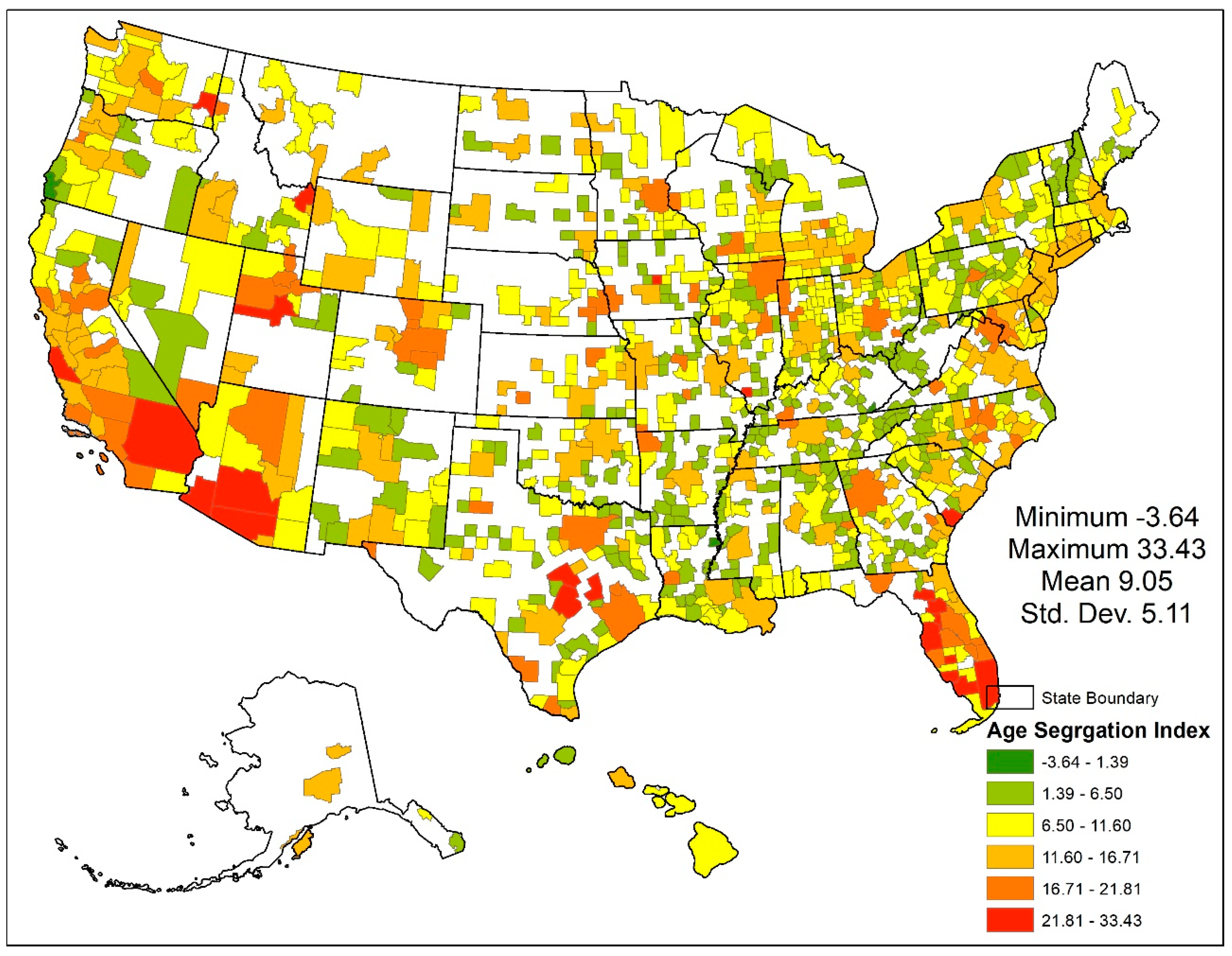
Our spatially explicit index shows that the degree of age segregation ranged from −3.6 (highly mixed) to 33.4 (highly segregated), with an average of 9.1 across the MMSAs. There were 86 out of 942 MMSAs above 1.5 standard deviations (16.7) and thus considered as highly segregated by age. Most of them were located in Florida, Texas, Arizona, and California (Figure 2), such as the Cape Coral–Fort Myers, FL, Riverside–San Bernardino–Ontario, CA, and Phoenix–Mesa–Scottsdale, AZ, metropolitan areas, possibly due to popular retirement destinations. Many urban areas in the Great Lakes and northeastern regions have low index values, indicating a more age-mixed residential pattern. A list of 25 MMSAs with the highest and lowest age segregation indices can be found in the Supplementary Materials.
3.2. Descriptive Statistics of Respondents Aged 65+ Years
Among the 92,560 respondents aged 65 years and above, almost two-thirds of these respondents were female, and more than 85% of respondents selected ‘white’ as their preferred race (Table 3). The racial distribution was close to that of the US Census 2010 (84.4% for white, 8.5% for black, and 3.4% for Asian among those aged 65+ years). On average, the male respondents reported higher income and education levels than their female counterparts, which is also consistent with the distributions from the US Census 2010. A majority (62.6%) of the male respondents were ‘married’ (versus 71.7% in the US Census 2010), while 44.3% of the female respondents were ‘widowed’ (versus 39.9% in the US Census 2010). As shown in Figure 1, every state in the US has at least two MMSAs with SMART samples so that the geography of older adults was well represented as well. This dataset, therefore, provided a large sample set with a good demographic representativeness and a wide geographic coverage for subsequent tests.
3.3. Global (Overall) Associations between Age Aggregation and Senior Health
Table 4 only summarizes the outcomes from Model 4 that include both individual-level and MMSA-level variables. The outcomes from the other three models can be found in the Supplementary Materials. At the individual level, men were less likely to report ‘good or better’ general health status as compared with women, but they experienced fewer mentally unhealthy days during last 30 days. Relative to those who identified as white, the respondents who identified as black or as other races reported worse health statuses. Lower levels of educational attainment and household income = decreased the likelihood of being in a ‘good or better’ health status and increased the days of feeling mentally and physically unhealthy.
At the MMSA level, we found that the spatial age segregation was not significantly associated with the elderly’s general health status (GENHLTH) and had no association with the days of physically unhealthiness (PHYSHLTH) either. This is consistent with previous arguments that there is no association between age segregation and elderly health by Aneshensel et al. [13] and Hybels et al. [14]. However, the Poisson mixed model indicates that the spatial age segregation was positively, although weakly, associated with the number of days of mental unhealthiness (MENTHLTH). That is, a one degree increase in a MMSA’s age segregation is associated with a slight increase (0.8%) in the number of ‘mentally unhealthy’ days. This echoes previous theoretical and empirical studies that argued the adverse effects of age segregation due to inadequate social support and ageism from the youth, leading to mental health issues in older adults [7,8]. The absence of interaction between the young and old could contribute to prejudices on each side about the other and a fear of growing older. In addition, separation also leads to missed opportunities, including the chance for older people to find happiness and a sense of purpose. With respect to the other MMSA variables, the percentage of the population without a high school diploma is negative associated with older adults’ health statuses but positively related to the number of unhealthy days. Although these global statistical tests suggest no or weak associations between spatial age segregation and senior health, these findings could be averaged effects across the country and may mask strong local patterns of associations. A local regression analysis, therefore, was necessary to offer more information.
3.4. Local Patterns of Associations between Age Aggregation and Senior Health
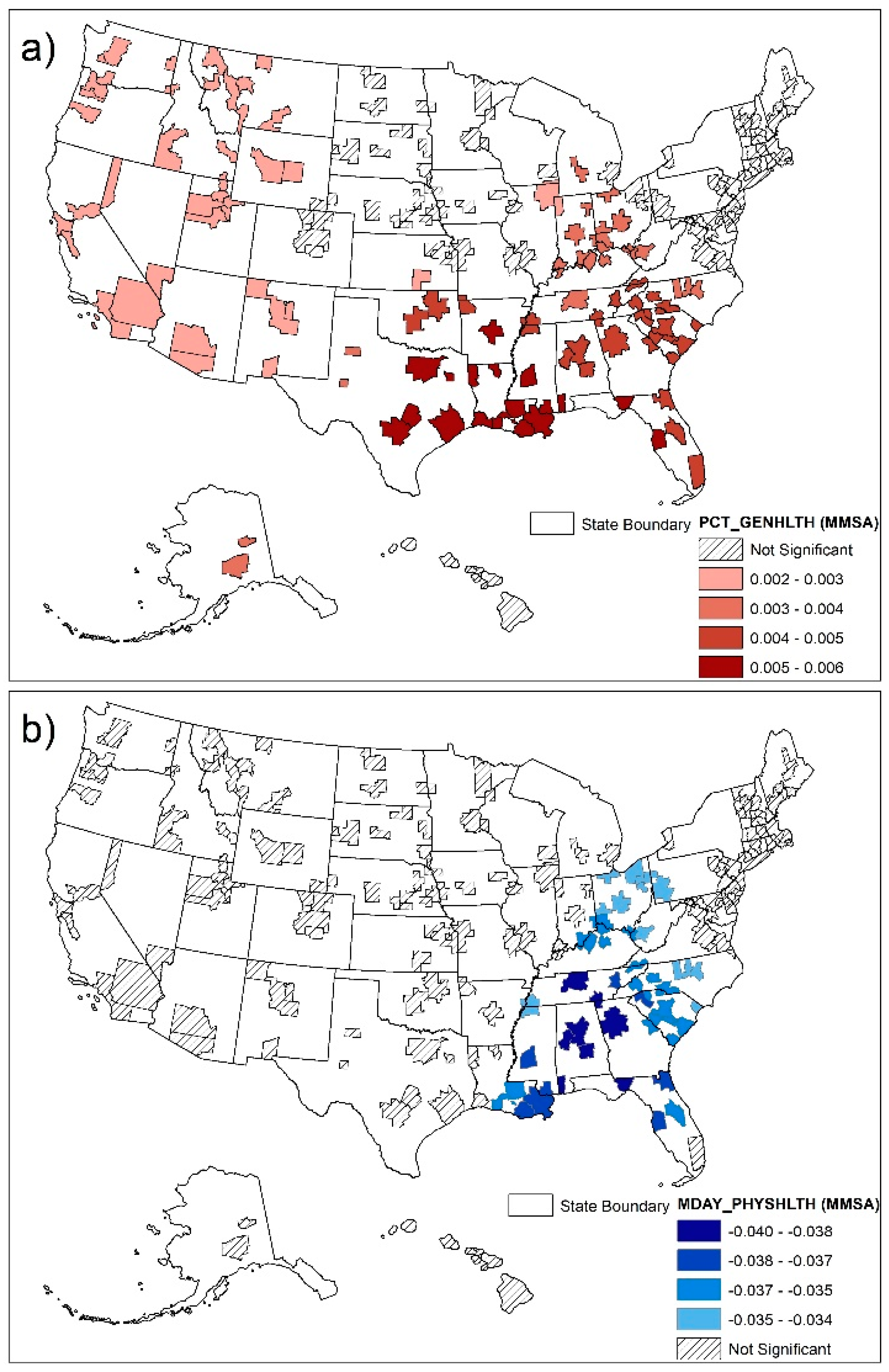
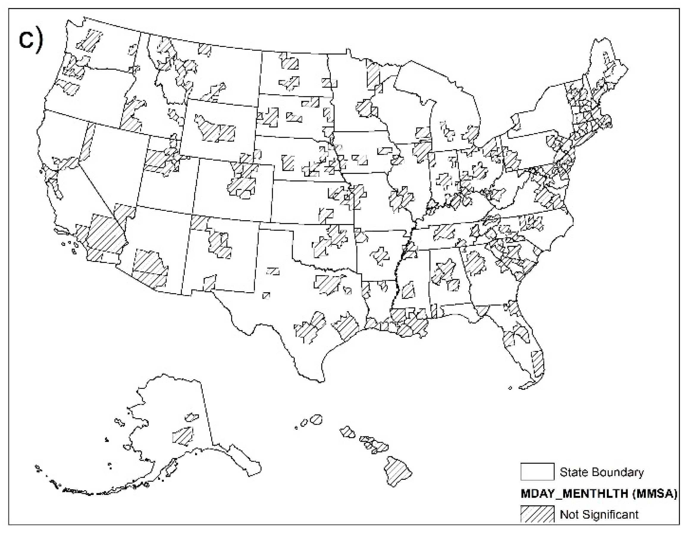
Figure 3 shows geographic or local patterns of associations between age segregation in MMSAs and the self-rated health of older adults across US cities, controlled by the racial structure, total area, education, and poverty levels of cities. We found several inconsistencies between global and local patterns of associations. For general health, although no global association was found, Figure 3a identified positive associations between the age segregation index and the likelihood of reporting ‘Good or Better’ general health (PCT_GENHLTH) in western and southern MMSAs but not in midwestern and northeastern MMSAs. For physical health, the global regression analysis suggested no significant association between age segregation and the days of being ‘physically unhealthy’ (Table 4), but Figure 3b identified a spatial cluster of significant negative associations in the southeastern region of the US. The average number of ‘physically unhealthy’ days (MDAY_PHYSHLTH) is fewer if a MMSA is more age-segregated. For mental health, while the global analysis suggested an overall positive association between the age segregation index and the days of being mentally unhealthy (Table 4), the local analysis implied no significant associations (Figure 3c).
4. Discussion
4.1. Spatially Explicit Age Segregation Index for MMSAs
In general, the resulting geographic patterns of age segregation (Figure 2) are consistent with the findings reported by Cowgill (1978). We further explored factors related to age segregation (the Supplementray Materials) and found that both the population growth rate of MMSA (2000–2010) and the size of MMSA had significantly positive correlations with the degree of age segregation. As previouly aruged by Cowgill (1978), fast population growth encourages differentiation and ecological specialization by age. Meanwhile, large-size metroloplitan areas provide sufficient room to accommandate territorial differentiation by age and stage of the family life cycle.
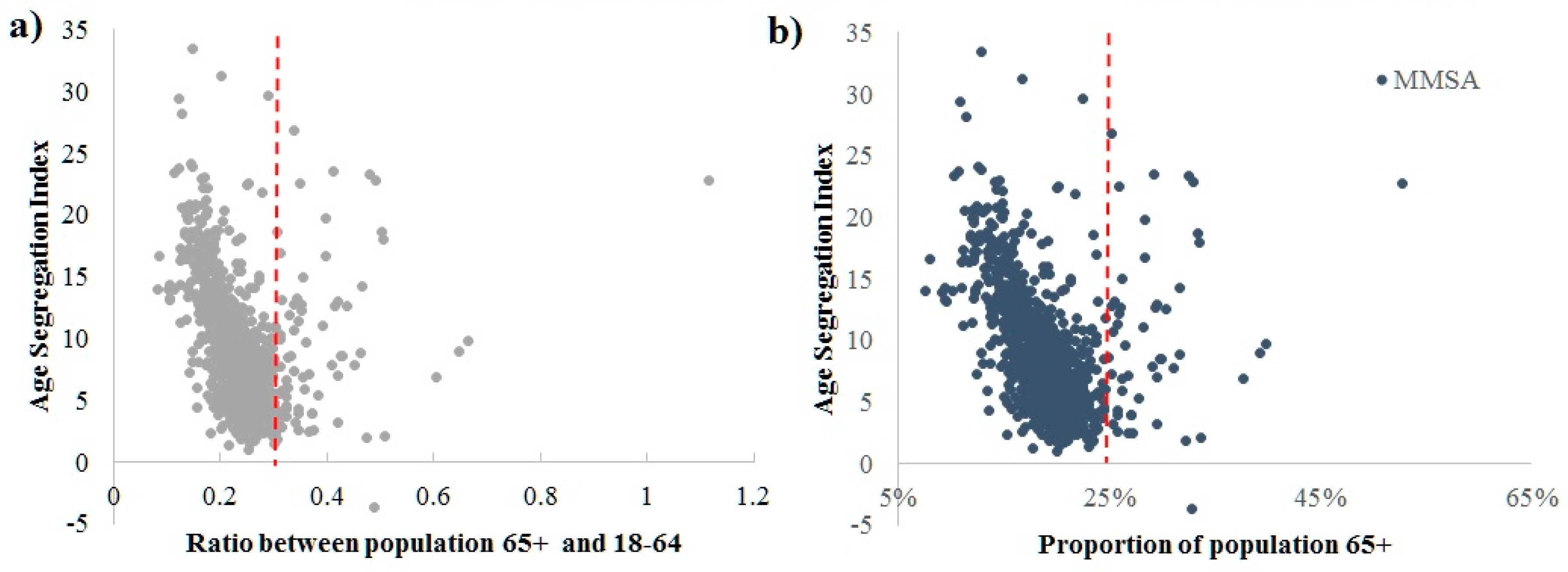
To show differences, we compared the spatial age segregation index for the MMSAs to two conventionally used age composition indices: the senior–adult ratio (population aged 65+ years to population aged 18–64 years) and the proportion of those aged 65+ years in the total population (Figure 4). When the senior–adult ratio is below 0.3 or the proportion of those ages 65+ years is under 25%, there is a strong negative correlation between age segregation and age composition. The age composition indices thus could be a reasonable proxy for cities that are disproportionally young, for example, college towns and fast-growing cities. The correlations become obscured as the age composition indices increase. For some cities with a relatively old population structure, for instance, cities popular for retirement destinations, the age composition indices are not good indicators for the degree of age segregation. Figure 4 demonstrates our early argument that the spatial arrangement of residents plays an important role in age segregation. Simply using non-spatial age composition indices can bias actual spatial patterns of age segregation and mislead the test for associations.
4.2. Associations between Age Aggregation and Senior Health
Inconsistencies between global and local regression analyses offer interesting insights for in-depth studies, for example, spatial clusters of local associations that might be otherwise masked in global regression analysis. Figure 3a,b consistently identified spatial clusters in the western and southern US, where age-segregated MMSAs are related to a higher proportion of seniors with ‘good or better’ general health statuses or fewer days of being physically unhealthy, in short, a better quality of health in older adults. This was not found in our global regression analysis. A possible reason lies in the geographic heterogeneity of the age segregation process (i.e., the age segregation was faster and more intense in the South and West (the so-called ‘snowbird migration’) as compared with other regions in the US, due to geographic factors, such as climate and urban growth). The retirement communities and healthcare facilities, thus, were more developed and concentrated to offer older adults a better living environment. The Villages and Sun City Center in Florida are good examples of those well-developed environments for the elderly to live together. Furthermore, these inconsistencies between the global and local analyses emphasize the need for region-specific investigation at an individual level (instead of at the MMSA level) to confirm local associations. For instance, the ‘no effect’ findings from other local observational studies in North Carolina [14] and Chicago [29] demonstrated our results from the local analysis on mental health, which led us to rethink the validity of global association.
From the perspective of policies to improve senior health, one-size-fits-all policies cannot be effective, and the policy designs need to be geographically adaptable. Those maps in Figure 3 would be critical references that provide details about where precise interventions should be targeted within each MMSA. For instance, city governments in the South and Middle West could offer incentives to senior people and encourage them to relocate, thus expediting the age segregation process for better general and physical health. On the other hand, the same policy might not be effective in other regions of US, where the underlying process of age segregation is different.
Our study does not attempt to either support or oppose age segregation in US cities. Instead, we advocate the use of a spatially explicit approach to analyze age segregation and senior health. For health policy makers and researchers on senior health, we proposed using a spatially explicit age segregation index to measure residential age segregation, instead of the statistical age composition. In our case study, we calculated the spatial age segregation index at the MMSA level to match the SMART data, but this index can also be estimated for census tracts using census block groups nested within them. Second, the use of SMART sample data has its strengths and weaknesses. The data is collected annually by the CDC and is publicly available for researchers. It also has a large sample size (over 90,000 older adults) and covers most major cities in the US, thus achieving good statistical and geographical representativeness. Its weakness lies in the limited information regarding the respondents’ residential locations, which are only available at the MMSA and county levels, in order to protect individual privacy. We only know whether respondents lived in an age segregated or mixed metropolitan area, but within that metropolitan area, we cannot infer the level of segregation of their neighborhoods (e.g., census tracts or ZIP codes). This prevented us from examining the associations at a finer scale, such as the census tracts used in many other studies. Our conclusions are subject to the modifiable areal unit problem (MAUP; i.e., the associations we found in this research are limited to the MMSA level and might not be applicable to finer geographic levels). Nevertheless, the SMART data could provide a quick pilot study before an in-depth investigation. Third, the GWR analysis could reveal spatially varying associations that were otherwise masked by conventional global regression analysis. While the conventional global regression answers whether there is an association across a study area, the local GWR analysis identifies where such an association may occur in the study area. In our study, although the GWR was limited to the MMSA level to accommodate the SMART data, it can also be adapted to finer scales, such as census tracts, if the sample data offer sufficient details. The GWR could be a useful tool for researchers to quickly identify spatial areas of interest and target their research efforts to validate local associations, which in turn offer more valuable insights into intervention than those from a conventional global analysis alone.
5. Conclusions
Americans are becoming increasingly segregated by age in this century. Does that contribute to good or bad health for senior people? At least, the analytical results from this nationwide study suggest that the associations are not very significant across the country but could be geographically clustered. The research on age segregation in modern America remains relatively young [3,30]. We contribute to the body of literature by advocating for the use of a spatially explicit metric and a spatially dependent analytic method. First, we stressed the necessity of using a spatial age segregation index to measure residential age segregation. By accounting for the spatial arrangement of residents in a city, this index is more reliable for investigating associations between age segregation and senior health. Second, we emphasized the need to recognize local variations of association between age segregation and senior health over a geographic space, which may not be identified in conventional global regression analysis. We proposed to combine global regression and local GWR analysis together to better understand and map the influence of age segregation. The proposed approach and findings could add new insights into the ongoing debate on practical issues regarding aging in place, such as urban planning, retirement investment, and health policy making.
Supplementary Materials
The following are available online at https://0-www-mdpi-com.brum.beds.ac.uk/2220-9964/7/9/351/s1, Table S1: 25 MMSAs with Most Age Segregation Index and 25 with Least Age Segregation Index, 2010. Figure S1: Scatterplot of age segregation index vs. MMSA growth rate 2000-2010. Statistical test shows that the correlation between them is significantly positive. Figure S2: Scatterplot of age segregation index vs. logarithm of area of MMSAs. Statistical test shows that the correlation between them is significantly positive. Table S2. Multilevel Models Predicting Variation in MENTHLTH among Elderly Populations. Table S3. Multilevel Models Predicting Variation in PHYSHLTH among Elderly Populations. Table S4. Multilevel Models Predicting Variation in GENHLTH among Elderly Populations.
Author Contributions
Conceptualization, L.M.; Data curation, G.D.; Methodology, L.M.; Formal analysis, G.D.; Writing—original draft, L.M.; Writing—review & editing, G.D.
Funding
This research was funded by the University of Florida Informatics Institute Seed Fund 2016.
Conflicts of Interest
The authors declare no conflict of interest.
References
- Ortman, J.M.; Velkoff, V.A.; Hogan, H. An Aging Nation: The Older Population in the United States. Available online: https://www.census.gov/library/publications/2014/demo/p25-1140.html (accessed on 1 August 2018).
- Golant, S.M. Aging in the right place. CSA J. 2015, 1, 61–62. [Google Scholar]
- Hagestad, G.O.; Uhlenberg, P. Should we be concerned about age segregation?: Some theoretical and empirical explorations. Res. Aging 2006, 28, 638–653. [Google Scholar] [CrossRef]
- Lagory, M.; Ward, R.; Juravich, T. The age segregation process: Explanation for american cities. Urban Aff. Rev. 1980, 16, 59–80. [Google Scholar] [CrossRef]
- Winkler, R. Research note: Segregated by age: Are we becoming more divided? Popul. Res. Policy Rev. 2013, 32, 717–727. [Google Scholar] [CrossRef]
- Moorman, S.M.; Stokes, J.E.; Morelock, J.C. Mechanisms linking neighborhood age composition to health. The Geront. 2016. [Google Scholar] [CrossRef] [PubMed]
- Addae-Dapaah, K. Age segregation and the quality of life of the elderly people in studio apartments. J. Hous. Elder. 2008, 22, 127–161. [Google Scholar] [CrossRef]
- McHugh, K.E.; Larson-Keagy, E.M. These white walls: The dialectic of retirement communities. J. Aging Stud. 2005, 19, 241–256. [Google Scholar] [CrossRef]
- Vogelsang, E.M.; Raymo, J.M. Local-area age structure and population composition. J. Aging Health 2014, 26, 155–177. [Google Scholar] [CrossRef] [PubMed]
- Glass, A.P.; Vander Plaats, R.S. A conceptual model for aging better together intentionally. J. Aging Stud. 2013, 27, 428–442. [Google Scholar] [CrossRef] [PubMed]
- Subramanian, S.V.; Kubzansky, L.; Berkman, L.; Fay, M.; Kawachi, I. Neighborhood effects on the self-rated health of elders: Uncovering the relative importance of structural and service-related neighborhood environments. J. Gerontol. Ser. B Psychol. Sci. Soc. Sci. 2006, 61, S153–S160. [Google Scholar] [CrossRef]
- Golant, S.M. In defense of age-segregated housing. Aging 1985, 348, 22–26. [Google Scholar]
- Aneshensel, C.S.; Wight, R.G.; Miller-Martinez, D.; Botticello, A.L.; Karlamangla, A.S.; Seeman, T.E. Urban neighborhoods and depressive symptoms among older adults. J. Gerontol. Ser. B Psychol. Sci. Soc. Sci. 2007, 62, S52–S59. [Google Scholar] [CrossRef]
- Hybels, C.F.; Blazer, D.G.; Pieper, C.F.; Burchett, B.M.; Hays, J.C.; Fillenbaum, G.G.; Kubzansky, L.D.; Berkman, L.F. Sociodemographic characteristics of the neighborhood and depressive symptoms in older adults: Using multilevel modeling in geriatric psychiatry. Am. J. Geriatr. Psychiatry 2006, 14, 498–506. [Google Scholar] [CrossRef] [PubMed]
- Maguire, A.; French, D.; O’Reilly, D. Residential segregation, dividing walls and mental health: A population-based record linkage study. J. Epidemiol. Community Heal. 2016, 70, 845–854. [Google Scholar] [CrossRef] [PubMed] [Green Version]
- O’SULLIVAN, D. Geographically weighted regression: the analysis of spatially varying relationships, by a. S. Fotheringham, C. Brunsdon, and M. Charlton. Geogr. Anal. 2003, 35, 272–275. [Google Scholar] [CrossRef]
- Cowgill, D.O. Residential segregation by age in american metropolitan areas. J. Gerontol. 1978, 33, 446–453. [Google Scholar] [CrossRef] [PubMed]
- Hagestad, G.O.; Uhlenberg, P. The social separation of old and young: A root of ageism. J. Soc. Issues 2005, 61, 343–360. [Google Scholar] [CrossRef]
- Office of Management and Budget (OMB). 2010 standards for delineating metropolitan and micropolitan statistical areas. Fed. Regist. 2010, 75, 37245–37252. [Google Scholar]
- Massey, D.S. Residential segregation and spatial distribution of a non-labor force population: The needy elderly and disabled. Econ. Geogr. 1980, 56, 190. [Google Scholar] [CrossRef] [PubMed]
- US Census. US Census Summary File 1. Available online: https://www.census.gov/prod/cen2010/doc/sf1.pdf (accessed on 1 August 2018).
- CDC Behavioral Risk Factor Surveillance System (BRFSS). Available online: https://healthdata.gov/dataset/cdc-behavioral-risk-factor-surveillance-system-brfss (accessed on 1 August 2018).
- Wong, D.W.S. Implementing spatial segregation measures in GIS. Comput. Environ. Urban Syst. 2003, 27, 53–70. [Google Scholar] [CrossRef]
- Duncan, O.D.; Duncan, B. A methodological analysis of segregation indexes. Am. Sociol. Rev. 1955, 20, 210–217. [Google Scholar] [CrossRef]
- Massey, D.S.; Denton, N.A. The dimensions of residential segregation. Soc. Forces 1988, 67, 281–315. [Google Scholar] [CrossRef]
- Morrill, R.L. On the measure of geographic segregation. Geogr. Res. Forum 1991, 11, 25–36. [Google Scholar]
- Bryk, A.S.; Raudenbush, S.W. Hierarchical Linear Models: Applications and Data Analysis Methods, 2nd ed.; Sage Publications: Thousand Oaks, CA, USA, 1992. [Google Scholar]
- Brunsdon, C.; Fotheringham, S.; Charlton, M. Geographically weighted regression. J. R. Stat. Soc. 1998, 47, 431–443. [Google Scholar] [CrossRef]
- Cagney, K.A.; Browning, C.R.; Wen, M. Racial disparities in self-rated health at older ages: What difference does the neighborhood make? J. Gerontol. Ser. B Psychol. Sci. Soc. Sci. 2005, 60, S181–S190. [Google Scholar] [CrossRef]
- Portacolone, E.; Halpern, J. “Move or suffer”: Is age-segregation the new norm for older americans living alone? J. Appl. Gerontol. 2014, 35, 836–856. [Google Scholar] [CrossRef] [PubMed]
Figure 1.
The study area, which contains 185 metropolitan and micropolitan statistical areas (MMSAs) reported in the 2011 Selected Metropolitan/Micropolitan Area Risk Trends (SMART) dataset. The color scheme indicates the number of respondents aged 65 years and above by MMSA. Those MMSAs without color were not reported in the SMART data for having less than 500 respondents.

Figure 2.
Spatially explicit age segregation index for 942 MMSAs across the US, based on the US Census 2010.
Figure 2.
Spatially explicit age segregation index for 942 MMSAs across the US, based on the US Census 2010.

Figure 3.
Local associations between MMSA-level age segregation and self-rated health in American older adults, controlled by the total area, poverty, and education levels. (a) PCT_GENHLTH, (b) MDAY_PHYSHLTH, and (c) MDAY_MENTHLTH.
Figure 3.
Local associations between MMSA-level age segregation and self-rated health in American older adults, controlled by the total area, poverty, and education levels. (a) PCT_GENHLTH, (b) MDAY_PHYSHLTH, and (c) MDAY_MENTHLTH.


Figure 4.
Comparison and correlation between the age segregation index and the age composition index, that is, the age segregation index versus (a) the ratio between seniors and adults; and (b) the proportion of senior people.
Figure 4.
Comparison and correlation between the age segregation index and the age composition index, that is, the age segregation index versus (a) the ratio between seniors and adults; and (b) the proportion of senior people.


Table 1.
Individual-level measures for self-rated health from the Behavioral Risk Factor Surveillance System (BRFSS) 2011.
Table 1.
Individual-level measures for self-rated health from the Behavioral Risk Factor Surveillance System (BRFSS) 2011.
| Theme | Variable Name | BRFSS Survey Question | Value | |
|---|---|---|---|---|
| Health Status at Present | General Health Status (GENHLTH) | Would you say that in general your health is…? | 1: Good or Better 0: Fair or Poor | |
| Healthy Days | Physical Health | Number of Days Physical Health Not Good (PHYSHLTH) | Now, thinking about your physical health, which includes physical illness and injury, for how many days during the past 30 days was your physical health not good? | Number of days from 0 to 30 |
| Mental Health | Number of Days Mental Health Not Good (MENTHLTH) | Now, thinking about your mental health, which includes stress, depression, and problems with emotions, for how many days during the past 30 days was your mental health not good? | Number of days from 0 to 30 | |
Table 2.
MMSA-level measures for health-related quality of life derived by aggregation *.
| Variable Name | Calculation | Value |
|---|---|---|
| Percent of General Health Status (PCT_GENHLTH) | Percent of respondents aged 65 years and above who reported a good or better general health in a MMSA | 0–100 |
| Average Number of Days Physical Health Not Good (MDAY_PHYSHLTH) | On average, how many days during the past 30 days a respondent 65+ in a MMSA felt physical health not good? | Number of days from 0 to 30 |
| Average Number of Days Mental Health Not Good (MDAY_MENTHLTH) | On average, how many days during the past 30 days a respondent 65+ in a MMSA felt mental health not good? | Number of days from 0 to 30 |
* All variables were adjusted by race.
Table 3.
Descriptive statistics of respondents aged 65 years and above.
| Gender | Male (35.8%) | Female (64.2%) |
|---|---|---|
| Race (%): | ||
| 1- White | 87.4 | 86.44 |
| 2- Black | 6.75 | 8.8 |
| 3- Asian | 1.95 | 1.86 |
| 4- Pacific Islander and others | 3.9 | 2.9 |
| Income level (%) | ||
| 1- <$15,000 | 7.84 | 16.12 |
| 2- $15,000–25,000 | 18.51 | 27.56 |
| 3- $25,000–35,000 | 14.70 | 16.97 |
| 4- $35,000–50,000 | 18.32 | 16.15 |
| 5- >$50,000 | 40.63 | 23.20 |
| Education level (%) | ||
| 1- Not graduate from high school | 10.14 | 10.85 |
| 2- Graduated from high school | 26.34 | 36.20 |
| 3- Attended college | 21.82 | 26.87 |
| 4- Graduated from college | 41.70 | 26.08 |
| Marital status (%) | ||
| 1- Married | 62.57 | 34.79 |
| 2- Divorced | 12.35 | 15.20 |
| 3- Widowed | 17.90 | 44.27 |
| 4- Separated | 1.34 | 1.01 |
| 5- Never married | 5.84 | 4.73 |
Table 4.
Multilevel models (Model 4) predicting variation in the self-rated health of older adults among US cities (the age segregation index as a continuous variable).
Table 4.
Multilevel models (Model 4) predicting variation in the self-rated health of older adults among US cities (the age segregation index as a continuous variable).
| GENHLTH | PHYSHLTH | MENTHLTH | |
|---|---|---|---|
| Intercept | 2.677 * | 0.896 * | 0.055 |
| Individual Level Variables | |||
| Gender | |||
| Men | −0.262 * | 0.017 | −0.174 * |
| Women (Ref.) | -- | -- | -- |
| Marital Status | |||
| Divorced/Widowed/Separated/Never Married | −0.019 | −0.003 | 0.018 |
| Married/Unmarried Couple (Ref.) | -- | -- | -- |
| Race | |||
| Other | −0.278 * | 0.016 | 0.127 |
| Black or African American | −0.361 * | −0.012 | −0.061 |
| White (Ref.) | -- | -- | -- |
| Education | |||
| Did Not Graduate High School | −0.950 * | 0.302 * | 0.276 * |
| Graduated High School | −0.454 * | 0.155 * | 0.100 * |
| Attended College or Technical School | −0.301 * | 0.159 * | 0.155 * |
| Graduated from College or Technical School (Ref.) | -- | -- | -- |
| Annual Household Income ($) | |||
| Less than 15,000 | −1.457 * | 0.864 * | 0.875 * |
| 15,000–25,000 | −0.998 * | 0.604 * | 0.560 * |
| 25,000–35,000 | −0.646 * | 0.393 * | 0.377 * |
| 35,000–50,000 | −0.366 * | 0.208 * | 0.258 * |
| Greater than 50,000 (Ref.) | -- | -- | -- |
| MMSA-level Variable | |||
| Age segregation index | 0.001 | 0.004 | 0.008 * |
| Total population | −0.000 | 0.000 | 0.000 * |
| Area (km2) | −0.000 | 0.000 | −0.000 |
| % of the population without high school diploma | −1.736 * | 1.132 * | 2.217 * |
| % of the population in poverty | −0.853 | −0.290 | −1.024 |
* indicates statistical significant at 0.05.
© 2018 by the authors. Licensee MDPI, Basel, Switzerland. This article is an open access article distributed under the terms and conditions of the Creative Commons Attribution (CC BY) license (http://creativecommons.org/licenses/by/4.0/).
Share and Cite
MDPI and ACS Style
Deng, G.; Mao, L. Spatially Explicit Age Segregation Index and Self-Rated Health of Older Adults in US Cities. ISPRS Int. J. Geo-Inf. 2018, 7, 351. https://0-doi-org.brum.beds.ac.uk/10.3390/ijgi7090351
AMA Style
Deng G, Mao L. Spatially Explicit Age Segregation Index and Self-Rated Health of Older Adults in US Cities. ISPRS International Journal of Geo-Information. 2018; 7(9):351. https://0-doi-org.brum.beds.ac.uk/10.3390/ijgi7090351
Chicago/Turabian StyleDeng, Guangran, and Liang Mao. 2018. "Spatially Explicit Age Segregation Index and Self-Rated Health of Older Adults in US Cities" ISPRS International Journal of Geo-Information 7, no. 9: 351. https://0-doi-org.brum.beds.ac.uk/10.3390/ijgi7090351
Note that from the first issue of 2016, this journal uses article numbers instead of page numbers. See further details here.