Exploring the Factors Driving Changes in Farmland within the Tumen/Tuman River Basin

Abstract

Understanding farmland changes and their mechanisms is important for food security and sustainable development. This study assesses the farmland changes and their drivers within the Tumen River of China and the Tuman River within the Democratic People’s Republic of Korea (DPR Korea) from 1991 to 2016 (1991–2000, 2000–2010, and 2010–2016). Farmland surfaces in Tumen/Tuman River Basin (TRB) for each of the years were mapped from satellite imagery using an object-based image segmentation and a support vector machine (SVM) approach. A logistic regression was applied to discern the mechanisms underlying farmland changes. Results indicate that cultivated surfaces changes within the two regions were characterized by large differences during the three time periods. The decreases of cultivated surface of −15.55 km² (i.e., 0.55% of total cultivated surface area in 2000) and −23.61 km² (i.e., 0.83% of total cultivated surface area in 2016) occurred in China between 1991 and 2000 and between 2010 and 2016, respectively; while an increase of 30.98 km² (i.e., 1.09% of total cultivated surface area in 2010) was seen between 2000 and 2010. Cultivated surfaces increased within DPR Korea side over the three time periods; a marked increase, in particular, was seen between 1991 and 2000 by 443.93 km² (i.e., 23.43% of total cultivated surface area in 2000), while farmland increased by 140.87 km² (i.e., 6.92% of total cultivated surface area in 2010) and 180.86 km² (i.e., 1.78% of total cultivated surface area in 2016), respectively, between 2000 and 2010 and between 2010 and 2016. We also found that expansions and contractions in farmland within both regions of the TRB were mainly influenced by topographic, soil, climatic, and distance factors, which had different importance degrees. Among these significant forces, the temperatures in the two regions were paramount positive factors on farmland changes during 1991–2016 and slope in China and precipitation in DPR Korea were the paramount negative factors affecting farmland changes, respectively. Additionally, except for between 2000 and 2010 in DPR Korea TRB region, most of the factors significantly influencing the farmland changes revealed the same positive or negative effects in different periods, because of mountainous topography. This study allows enhancing understanding of the mechanisms underlying farmland changes in the TRB.

1. Introduction

Land is the most basic natural resource and it provides the means for human survival and development [1,2]. Understanding land use and cover change (LUCC) is therefore critically important for assessing global environmental variation and sustainable development [3,4]; these factors significantly influence local, regional, and global climate change, ecosystems [5,6], and human welfare [7]. Cultivated land is the most essential component of this overall resource in the context of food security, but faces competition from land use demands for industrialization, urbanization, and ecological environmental construction [8]. General changes to farmland over time include expansion and contraction, both the result of reclamation by cultivate activities [9], farmland abandonment because of rural-to-urban population migration [10], and conversions associated with urbanization, industrialization, and ecological rehabilitation projects [11,12]. Previous work has shown that agricultural lands have generally expanded into higher latitude regions over recent decades as population levels have increased in concert with food demand and global warming [13]. The area of farmland in mountainous areas of Europe and Japan has continuously contracted since the late 1980s because of abandonment [10]; similarly, large areas of cropland across some regions of China have also contracted over the last 20 years, mainly converted to built-up areas, forests, and grassland via urbanization activities and ecological restoration projects [14].

Mountain regions tend to be more sensitive to LUCC [15] and farmland dynamics in these areas are also complicated by the multiple impacts of terrain, spatial heterogeneity, and land use policies [16]. Understanding farmland changes (both expansion and contraction referred to the cultivated surface) and their underlying driving factors is therefore important for modeling future dynamics, developing food security management strategies, and sustainable development. Studies have shown that the major driving forces affecting farmland changes include physical (e.g., slope, elevation, aspect, soil properties and type), socioeconomic (e.g., population density, foreign labor migration, farmer incomes, and gross domestic product, gross domestic product (GDP)), climatic (e.g., mean annual temperature and precipitation), and distance factors (e.g., distances to roads, rivers, and settlement) [3,10,15,17]. The relative influence of these variables on farmland changes may, however, take place at different rates and at various stages [15] in different regions and time periods. A range of neural network models [18] as well as analytic hierarchy process-based approaches [19], multivariate regression models [8], principal component analysis [16], and canonical correlation analysis [20], alongside logistic regression (LR) models [21,22], have been utilized in this field to estimate the forces driving LUCC. In terms of spatial sampling (SS), LR models have been widely applied to estimate the quantitative relationship between the spatial distribution of LUCC and driving forces by incorporating physical, socioeconomic, climatic, and accessibility factors [22,23,24]. However, most previous studies to address forces driving farmland changes mainly concentrated on the problems of either farmland expansions or contractions, and deeper studies for forces underlying farmland expansions, as well as contractions, are lacking. Individual analysis of the different factors leading to both expansions and contractions in farmland status is important for the deeper understanding of such changes in mechanisms, and determining how farmland may be better managed in the future. Yu et al. (2017) [25] have successfully used a binary LR model to separately discern the driving forces underlying both expansion and contraction in greenhouse land, in Shouguang City, China.

The Tumen/Tuman River Basin (TRB) is a trans-boundary river basin in Northeast Asia that includes the international boundaries between China, the Democratic People’s Republic of Korea (DPR Korea), and Russia. Because of the geographic location of this region as well as climate change, population growth, and socioeconomic development, overall LUCC within the TRB has been noticed in recent years; farmland area in particular has been substantially changed within this region due to increasing human demands for biological resources [26]. Arable land in China, which has a large population, the rapid growth of population and economic development is scarce, and agricultural industry faced a scarcity of land and urgent food security [12]. Even in DPR Korea arable land is scarce, because nearly 80% of the country’s territory is covered by mountainous forests, and repeated natural disasters since the 1990s have remarkably reduced agricultural productivity [27]. Additionally, agricultural lands are easily meeting the demands of land use for industrialization and urbanization, as well as ecological environmental construction [8]. Therefore, farmland contractions by industrialization and urbanization, as well as the extensions in farmland by land reclamation can cause threats to food security, as well as sustainable development. As food security is fundamental for two countries, and farmland area in TRB has been substantially changed, the studying forces driving farmland changes are an issue that need to be focused on in our study area, for food security and sustainable development. However, it remains poorly understood in this area. Estimating the key factors that influence changes in farmland will, therefore, provide the valuable information for government planning and management activities on farmland in the Chinese and DPR Korea zones.

The objective of this research was therefore to investigate the factors driving farmland changes within Chinese and DPR Korea regions of the TRB between 1991 and 2016. Thus, the specific objectives of this research are to generate a series of cropland maps across the study area for 1991, 2000, 2010, and 2016, to assesses the spatiotemporal expansion and contraction of farmland within different TRB regions throughout these three periods using a series of Landsat images, and to estimates the combination of drivers and their relative importance to farmland changes within different regions during the three periods.

2. Materials and Methods

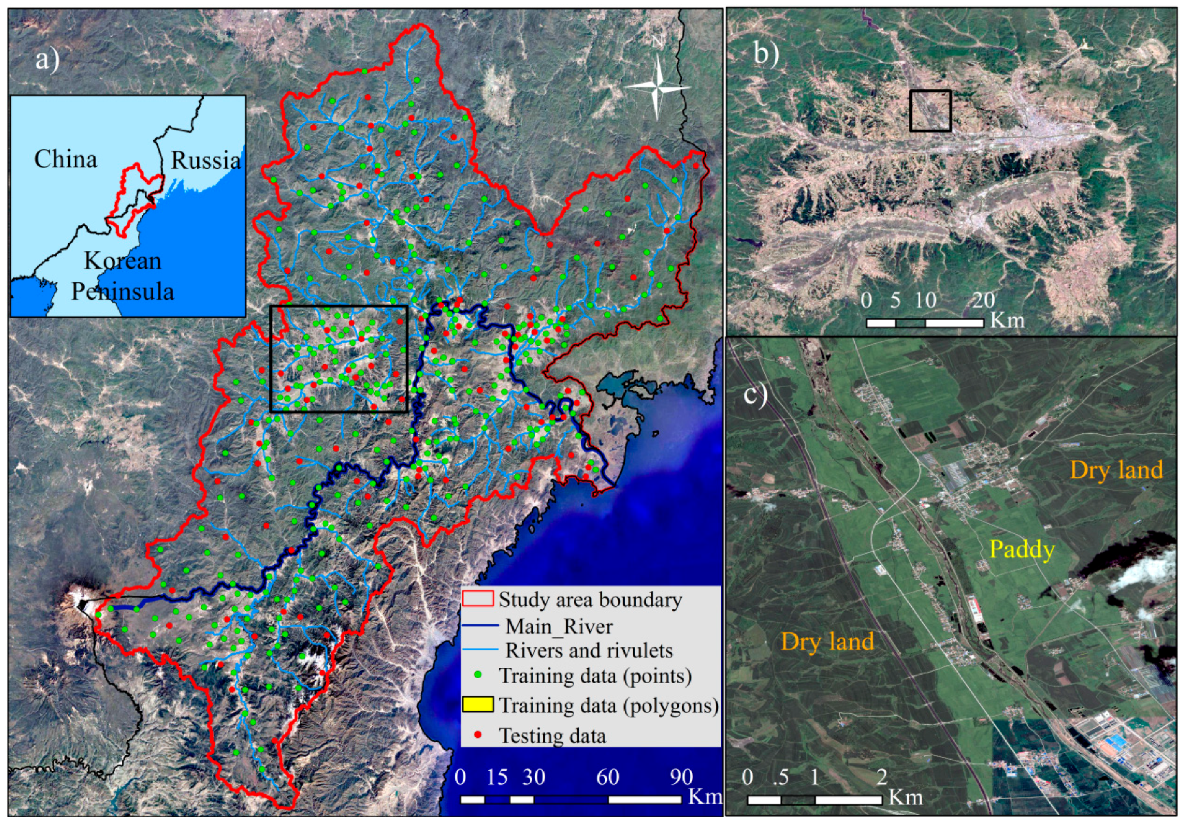
2.1. Study Area and Overview of the Study

The zone studied here encompassed an area of 30,598 km², including both DPR Korea and Chinese TRB regions, which comprise approximately 10,133 km² and 20,464 km², respectively. The TRB is located within latitudes between 40°86′ N and 44°32′ N and longitudes between 127°70′ E and 132°09′ E in northeast Asia, which comprises the international boundaries between the Korean peninsula, China, and Russia (Figure 1a); however, our study area did not include the Russian region of the TRB (an area of about 3480 km²) because it encompasses a very small area of farmland. The a main river comprises a length of 525 km, and it originates in the eastern mountainous foothills of Mt. Paektu on the DPR Korea side [28], and enters into the East Sea of Korea [29]. This basin includes numerous tributaries that flow into the river, and the overall TRB experiences a typical temperate monsoonal climate [28,29] with an annual mean precipitation (AMP) between 400 mm and 650 mm, and an annual mean temperature (AMT) between 2 °C and 6 °C [30]. The elevation across the region also increases from east-to-west and from north-to-south, and it includes plains and mountains; the major land use types include forested land, farmland, grassland, urban land, water bodies, and barren land. The farmland area across the entire study region was about 4886 km² in 2010, which mainly included dry land and paddy fields (Figure 1b,c).

We estimated the driving forces on farmland changes within the different two regions of TRB between 1991 and 2000, between 2000 and 2010, and between 2010 and 2016. Data collection was firstly performed according to this study requirement, which included satellite remote sensing (RS) data and potential driving force data. After pre-processing of all the obtained data, four land cover types for the study area were produced by using the combined object-based image segmentation and support vector machine (SVM) supervised classifier. These land cover maps were then grouped into two categories including farmland and other land, and they were also overlapped by groupings into 1991 and 2000, 2000 and 2010, and 2010 and 2016, to estimate the farmland changes, and to produce the change maps (i.e., expansion and contraction maps). All farmland change maps were coded as binary value 1 (for expanded areas in expansion maps or for contracted areas in contraction maps) or 0 (for unchanged/other land areas in expansion or contraction maps). In order to estimate the forces driving farmland changes within different regions of TRB, statistical analyses such as SS, Z-Score standardization (ZS), multicollinearity test (MLT) and LR modeling were individually performed in different regions of the TRB (see Section 2.3). Finally, we analyzed the mechanisms on farmland expansion or contraction in different region levels, from the LR model results. The general framework of this study is illustrated in Figure 2.

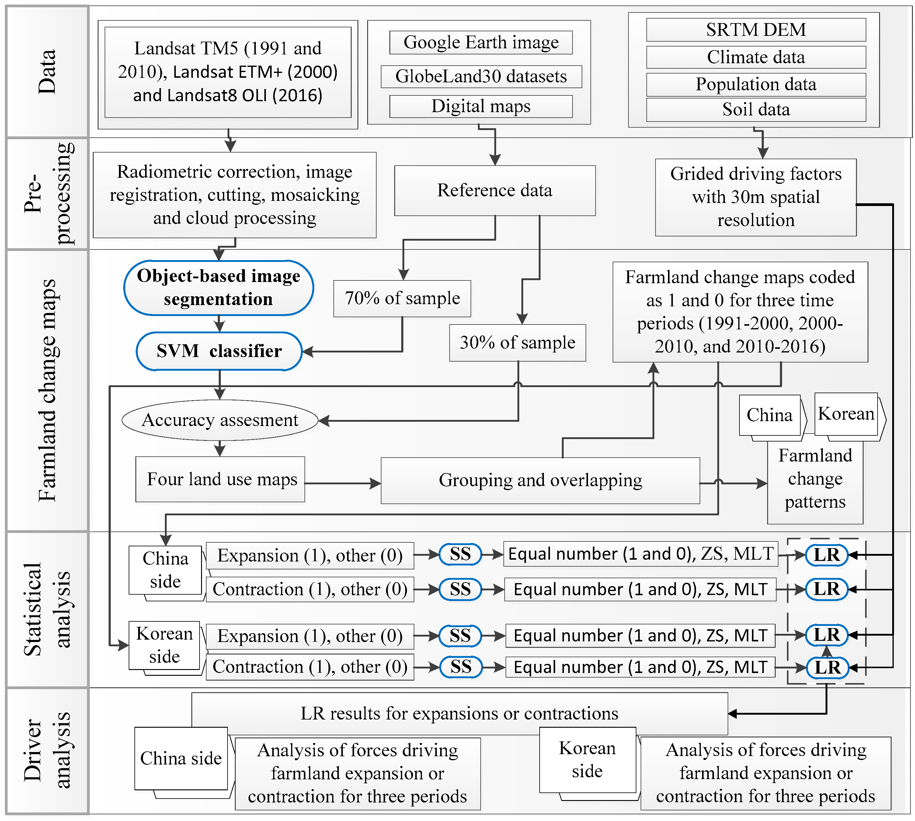
2.2. Data Sources and Data Processing

2.2.1. Data Sources

RS data have been widely utilized to create maps for evaluating and monitoring LUCC. We utilized Landsat TM, ETM+, and OLI satellite images for 1991, 2000, 2010, and 2016 in this study, which had a spatial resolution of 30 m, as shown in

Table 1. Details of the satellite data used *.

Year	Sensor	Path/Row	Date	Year	Sensor	Path/Row	Date
1991	TM5	114/30	8 October 1991	2010	TM5	114/30	6 June 2010
	TM5	115/30	17 October 1992		TM5	115/30	3 September 2009
	TM5	115/31	29 September 1991		TM5	115/31	30 September 2009
	TM5	116/30	31 May 1991		TM5	116/30	24 September 2010
	TM5	116/31	31 May 1991		TM5	116/31	24 September 2010
2000	ETM+	114/30	25 September 2001	2016	OLI	114/30	21 May 2016
	ETM+	115/30	24 May 2000		OLI	115/30	11 June 2015
	ETM+	115/31	24 May 2000		OLI	115/31	28 May 2016
	ETM+	116/30	2 September 1999		OLI	116/30	19 May 2016
	ETM+	116/31	2 September 1999		OLI	116/31	19 May 2016

* Satellite data for 22 September 1992 (Path/Row; 116/31), 29 September 2000 (115/30), 18 October 2001 (115/31), 9 October 2009 (114/30), 4 September 2011 (115/30) and 14 June 2014 (115/30) were used to make cloud-free images from imagery in Table 1.

. These images were downloaded from the United States Geological Survey (USGS) website (http://earthexplorer.usgs.gov/) [15]. Bands 1–5 and 7 (Landsat TM & ETM+) and bands 2–7 (Landsat-8 OLI) were used for land cover classification. The historical Google Earth (GE) images and GlobeLand30 datasets of the national geomatics center of China for 2000 and 2010 [31] were used to correct the reference data for image classification and accuracy assessment of the final land cover maps.

Open-access Shuttle Radar Topography Mission (SRTM) 30 m resolution digital elevation model (DEM) data were also used to determine the longitude, latitude, elevation, slope, and aspect of the study area; all were downloaded from the USGS site. DEM data were also used to define the boundaries of the study area by applying the ‘hydrology tool’ in the software ArcGIS 10.3 software (Environmental Systems Research Institute, Redlands, CA, USA) [32].

Daily climate data (i.e., temperature and precipitation) were obtained from 21 meteorological stations across in and around the TRB. These data were provided from two service sources; one was the China Meteorological Data Interchange Platform (http://data.cma.cn/) for the Chinese region, and other is the National Oceanic and Atmospheric Administration (NOAA) National Centers for Environmental Information database (http://www.noaa.gov/) for the DPR Korea and Russia TRB regions. In order to produce AMT and AMP grid data with a spatial resolution of 30 m × 30 m across the whole study area, AMT and AMP values (i.e., for 1991–2000, 2000–2010, and 2010–2015) for each meteorological station were firstly calculated from daily climate data using the MATLAB R2014a software (The Mathworks, Inc., Natick, MA, USA) [33], respectively. Further, as topography is a key factor impacting temperature and precipitation [34]; multiple linear regression models were therefore applied using climate data (i.e., AMT and AMP) and topographic factors (extracted from SRTM DEM with 30 m-resolution) at the meteorological stations to make the linear regression relationships between climate factors and topographic factors. In the multiple linear regression models, the longitude, latitude, elevation, and distance from the nearest coastline were used as AMT-related independence variables, while the same set of variables plus slope and slope direction were selected as AMP-related independence variables. Using these regression models, climate values for each pixel were predicted to grid cells with a spatial resolution of 30 m × 30 m. The errors between observed and predicted climate factors were calculated for whole meteorological stations and error grids with a spatial resolution of 30 m × 30 were produced by interpolating errors using Kriging interpolation method. Finally, AMT and AMP with high accuracy were produced by summing predicted climate grids and error grids.

The soil property data used in this study were downloaded from the ISRIC world soil information website (http://isric.org/), all SoilGrids data based on global soil profiles and environmental covariate data, including physicochemical properties and classifications at a 250 m spatial resolution. Soil sand and clay contents were utilized here as potential factors to assess farmland changes; soil property data were converted at a 30 m × 30 m spatial resolution using the ArcGIS 10.3 software, while the river, road, and settlement data utilized in this study were obtained from historical GE images and a range of different digital maps using the Chinese software River Map (http://www.rivermap.cn/).

2.2.2. RS-Based Farmland Maps and Change Maps

Firstly, we developed a land use and land cover (LULC) classification system, which includes farmland (i.e., including paddy fields and dry land), forested land, grassland, settlements, water bodies, and barren land. Reference data for image classification and accuracy assessment were collected for different years across the study area, based on our classification system. The minimum number of reference pixels for each land cover type required the number of bands plus one. Reference points and polygons for 2010 were manually collected and digitized through visual interpretation on GE image and from GlobeLand30 land cover map in 2010 and digital maps (Figure 1a). During the generation of the reference data, we ensured that reference points or polygons were spatially disjointed. The adjustment and addition or removal of the reference data for 1991, 2000 and 2016 were then performed through visual interpretation on historical GE image in different years, based on reference data for 2010. The reference points for each year were randomly divided into two subsets; about 70% of reference samples (more 300 points and more 100 polygons) were used for training the classifier and the rest reference data (only points) were used to estimate the accuracy assessment of final farmland maps. In addition, as the pre-processing of satellite images was essential to this study, in these stages, we applied comprised radiometric correction (i.e., radiometric calibration and Fast Line-of-sight Atmospheric Analysis of Hypercubes (FLAASH) atmospheric correction), automatic image-to-image registration (i.e., images for 1991, 2000, and 2016 were all registered on the basis of 2010 image data), image cutting, mosaicking within the same season, and cloud area masking and replacement. Land use maps for 1991, 2000, 2010, and 2016 were then extracted from Landsat satellite images to generate farmland maps for different periods using object-based image segmentation and a SVM classifier. The SVM obtained a higher overall accuracy (OA) of 84.62% and 89.23% than the OA of 83.85% and 86.15% of the maximum likelihood classifier (MLC) for the TM and OLI images, respectively [35]. Additionally, an object-based SVM classifier showed a higher OA of 95% compared to the OA of 89% of MLC [36]. The key advantage of utilizing an object-oriented technique rather than a traditional pixel-based approach is that the various aspects of information as the basis for classification, such as texture, shape, and position characteristics can easily be calculated by segmenting the image. SVM [37] is a supervised classification technique based on non-parametric and non-linear statistical theory, and it can thus obtain good results from complex and noisy data [38]. A SVM classifier optimally separates the different classes of data by finding the hyperplane for optimal classification [36,39]. The hyperplane is the decision surface that is used to determine the optimal classification, and a good separation is achieved by the hyperplane that has the largest distance to the neighboring data points of both classes [40]. An optimum hyperplane is determined using a training sample dataset and its generalization ability is verified using a validation dataset [36]. SVMs for land cover classification have four kernel functions such as linear, polynomial, radial basis function (RBF), and sigmoid [41], which are mentioned in the help section of ENVI 5.1 software (Exelis Visual Information Solutions, Boulder, CO, USA) [33]. For more detailed kernel functions for SVMs for land cover classification, refer to the previous study of Kavzoglu et al. (2009) [42].

In this study, a RBF kernel was used for image classification because the RBF kernel can achieve better results than other kernels [41]. Image segment and merge parameters for object-based segmentation process were set at 30 and 70, respectively [43], and the image objects obtained from the segmentation procedure were classified using the SVM supervised classifier.

In order to achieve the main objective of this study, farmland maps for the four periods were finally produced by grouping land use maps, including both farmland and other land. Overlaying farmland layers for neighbor two years to assess expansion during three time periods studied, values for each raster were assigned as 1 if farmland in the next time period expanded, otherwise coded as 0, to denote the presence or absence of change (i.e., expansion) in farmland status. Similarly, to assess farmland contraction during different three time periods, values for each pixel were also coded as 1 if a change (i.e., reduction) had occurred, or otherwise coded as 0. This process enabled us to produce farmland change maps (i.e., farmland expansion and contraction maps) in binary form for each regional level across the study area; these farmland change maps were then used as dependent variables for LR analysis, after processing of SS.

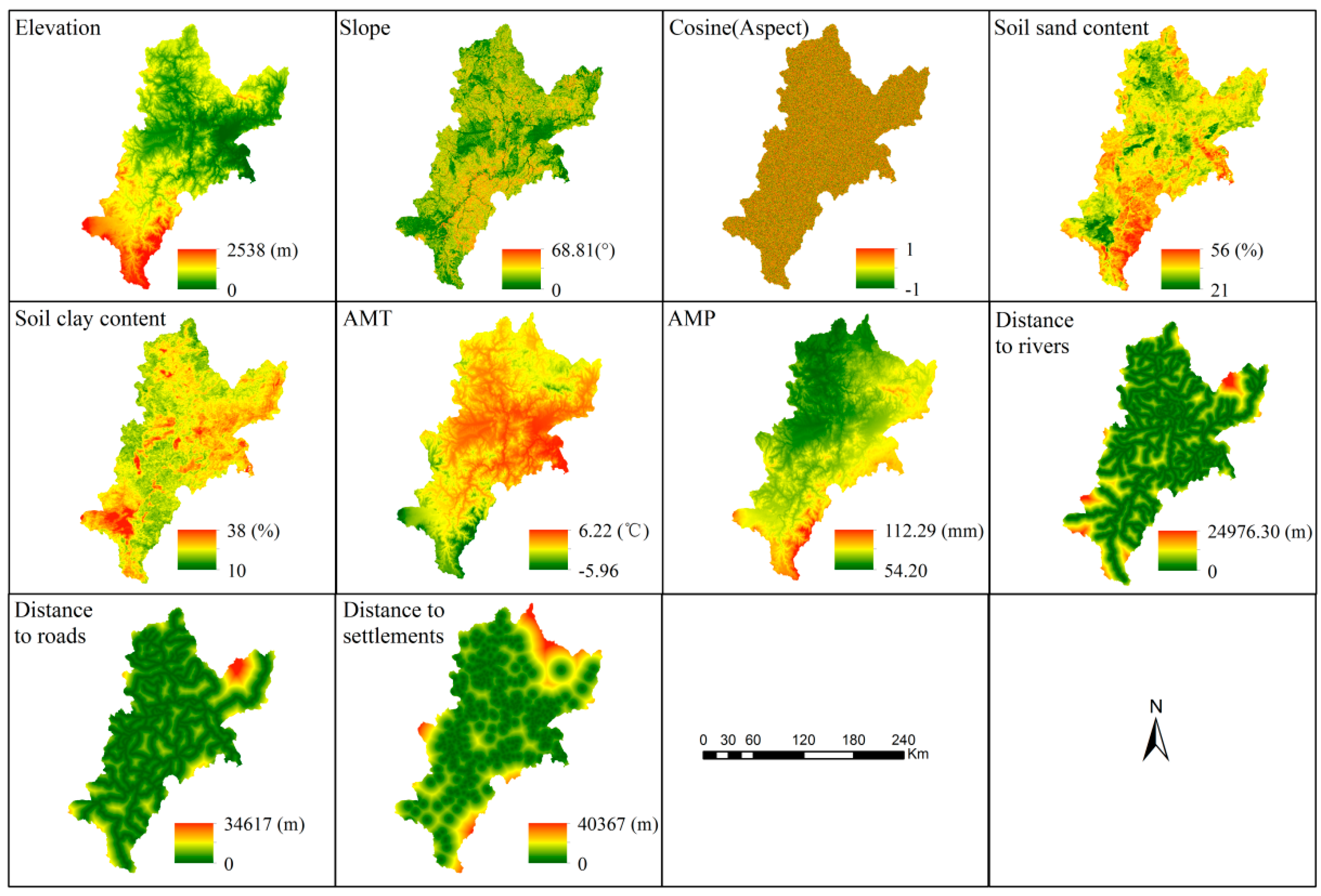
2.2.3. Selecting Potential Driving Forces

It is well-known that LUCCs are the result of natural and social factors, influences that are not the same at different regional levels. Corresponding data availability and previous research [15,22,44,45] reveals that distance (i.e., distances to road, rivers, and settlements), topography (i.e., elevation, slope, and aspect), soil (i.e., soil sand and clay content), and climatic factors (i.e., AMT and AMP) have all been hypothesized as potential explanatory driving forces underlying farmland changes (

Table 2. Factors used to describe farmland changes.

Category	Variables	Type (unit)
Topographic factors	Elevation	Continuous (m)
	Slope	Continuous (degree)
	Aspect	Continuous (cosine)
Soil factors	Soil sand content	Continuous (%)
	Soil clay content	Continuous (%)
Climate factors	AMT	Continuous (°C)
	AMP	Continuous (mm)
Distance factors	Distance to rivers and rivulets	Continuous (m)
	Distance to roads	Continuous (m)
	Distance to settlements	Continuous (m)

).

Elevation and slope have been considered to be the main topographical factors that influence farmland spatial patterns [3] and agricultural production, especially in mountainous areas [10]. Previous studies have also shown that these variables play important roles in determining land use [46], as regions with higher elevations and steeper slopes usually make production more difficult and lead to higher farmland and cultivation costs than their counterparts at lower elevations with more gentle slopes [47]. Similarly, aspect is also an important topographical variable that influences farmland, as rainfall and sunlight are correlated with aspect, and are both necessary for crop growth [3]. Elevation, slope, and aspect were therefore evaluated here using a DEM with a spatial resolution of 30 m. Because aspect is a circular variable, therefore, it cannot be measured in logistic regression. Cosine transformation was performed to obtain a continuous gradient (i.e., stressing the north-south or east-west gradient) from aspect being a circular variable [48]. The transformed cosine aspect values indicate that solar radiation condition is better if the value is closer to −1; otherwise it is lower. At the same time, soil properties (i.e., sand, clay, and silt contents) are also important variables that influence topsoil layer permeability; these property data are usually used to evaluate soil erosion as components of the revised universal soil loss equation [49]. Existing studies have also shown that soil erosion determines farmland abandonment [50]; lands with higher soil sand content are therefore more likely to be abandoned, which suggests that these regions are inclined to be abandoned as they are poor-quality [10]. Two soil sand and clay contents were therefore selected as variables in this analysis, to represent quality status.

Climatic factors can also be used to generate changes in vegetation growth and land use practices. We therefore selected AMT and AMP for 1991–2000, 2000–2010, and 2010–2015 as potential climate factors on farmland changes for different periods, respectively.

The distance factors selected in this study include distances to rivers, roads, and settlements. These factors were used to reveal the factors driving farmland changes in various previous studies [3,15]. The Euclidean algorithm was used to calculate all distances at a 30 m × 30 m spatial resolution in the software ArcGIS 10.3 software.

Driving forces across different spatial resolutions have different coupled results; it is therefore important to select the best spatial resolution for such studies [51]. We selected an initial 30 m spatial scale for Landsat TM image data (one pixel × one pixel). Thus, all factors with different spatial resolutions were converted to 30 m raster format (Figure 3) and exported as SPSS files format for LR analysis.

2.3. Statistical Analysis

This LR analytical approach is advantageous as it is very effective if the dependent variable is binary in form [52]. Thus, based on available driving factor data, study objects, and previous studies [15,22,25,52], a LR model based on SS was selected here to estimate the potential driving forces underlying farmland changes.

2.3.1. SS Procedure

It is noteworthy that once all pixels have been selected as regression samples, dependent variables have the potential to become spatially auto-correlated, a phenomenon by which their independence contravenes LR assumptions and leads to potentially biased results [25,52]. Indeed, as our data encompassed very large number of pixels (i.e., 9775 × 6323 and 7986 × 5587 grid cells for Chinese and DPR Korea TRB regions, respectively) for both dependent and independent variables, we faced particular challenges for spatial statistical analysis typical to correlational research [21,44,53]. These issues were addressed through the combined approach of systematic and random sampling [22]. While a LR model is interpreted as binary forms by the presence (i.e., 1 as true) or absence (i.e., 0 as false) of events [25,54], in our study, both expansion and contraction in farmland status were all events that represented the changes in farmland status. That is, the expanded areas in farmland expansion maps denoted the conversion of other land categories to farmland; the contracted areas in contraction maps also denoted the conversion of farmland to other types of land. Therefore, the presence of expansion or contraction in farmland status was denoted 1 and the absence of expansion or contraction indicated 0, in farmland expansion maps or farmland contraction maps, respectively. In addition, the dependent variable in a LR model requires the equal number of points, coded as 0 and 1. From the research objective and the principle of a LR model, we therefore separately applied a combined systematic and random sampling approach for expansion or contraction in farmland status within different two region levels, to solve the above mention two issues (i.e., a spatial auto-correlation and big data processing problems) [17,52] and to obtain the dependent variable with the same number of codes, 0 and 1, in a LR model.

For example, for farmland expansion, the systematic sampling was done on the farmland change map, coded as 1 (expansion areas) and 0 (other areas) at the end of each time period, after farmland area within a base year was removed from the above farmland change map to ensure the LR model’s accuracy [22]. However, in this study, as the number of points coded 0 were much larger than those coded as 1 [44], we therefore performed random sampling for the only systematic sampled points within other land categories (coded as 0) to ensure that these were equal to the sample points from expansion areas (coded as 1) to estimate unbiased parameters [44,55]. An equal number of points coded 0 and 1 were therefore acquired; thus, for different periods and county levels, the number of sampling points was set at 30%, based on the results of previous work [25]. These sampling points were then used to extract the pixel values of dependent (farmland expansion) and independent (driving factors) variables from farmland change maps, and all driving factor layers in each period for subsequent LR analysis. The SS procedures for farmland contractions were also performed by using the sameness method with that for expansion in farmland.

2.3.2. Running of the LR Model

The LR model is a method that can be used to discover the interrelated relationships between a binary dependent variable, and several independent categorical and continuous variables [51,56]. This approach has been used extensively to examine the relationship between land use probability and driving forces, as it can predict the occurrence probability of an event under the control of multiple independent variables, using a mixture of continuous and categorical variables [51,56,57,58]. Therefore, a binary LR model can quantitatively discern the mechanisms underlying the expansion as well as the contraction in land cover, respectively [25]. The binary LR formula used in this study is:

$$Y=\log \left(\frac{P}{1-P}\right)={\beta }_0+{\beta }_1{X}_1+{\beta }_2{X}_2+{\beta }_3{X}_3+\dots +{\beta }_n{X}_n,$$

(1)

In this expression, the dependent variable ($Y$) has the binary value, 1 or 0 which denotes the presence or absence of farmland expansion or contraction [25]. $P$ denotes the occurrence probability of a cell being subject to farmland expansion or contraction, ${\beta }_0$ is the constant to be estimated, ${\beta }_1,{\beta }_2,{\beta }_3\dots ,{\beta }_n$ are partial regression coefficients of predictor variables, $X_j(j=1\cdots n)$ indicates the j-th independent variables (i.e., driving forces), and n represents the total number of factors.

Prior to performing the logistic regression, the standardization processing and multicollinearity test for the independent variables are important to fit the binary logistic regression. All independent variables were standardized using the Z-score standardization method to reduce the disparities in scale of measurement and variance, because of different units of the variables. For these standardized variables, a multicollinearity test was conducted to avoid multicollinearity between independent variables by using the variance inflation factor (VIF) analysis [59]; variables with significant collinearity (VIF ≥ 10) must be removed from the LR model. These Z-score methods and multicollinearity analysis were performed in SPSS, and results shown that all independent variables were required to enter into LR model. Subsequent to the generation of a LR model using the software SPSS, output regression coefficients and model parameter estimates were generated, including the Wald statistic ($\chi 2$), Nagelkerke R², overall percentage correctly predicted (PCP), and the significance of the probabilities. Amongst these, the Wald statistic values are useful for judging the relative weights of each explanatory variable in a LR model, and they can be used to evaluate the contribution of each explanatory variable in event-prediction [17,25]. This means that higher Wald statistic values for an independent variable are the most important LUCC variables; these values have been widely used to assess the relative importance of each driving factor in such studies [10,17,59]. Variables in each LR model were therefore selected if they were statistically significant at a p-value less than 0.05, while Nagelkerke’s R² values (between 0 and 1) in each logistic model were used to test the goodness of fit. A good logistic model fit was defined for each value of 0.2 and above [59], while relative operating characteristics curves have commonly been used to validate LR model performance; the area under the curve (AUC) was connected via plotted points [44], including values between 0.5 and 1 [51]. A value higher than 0.9 was considered as a high value, while one between 0.7 and 0.9 was credible, and a value that was less than 0.7 was considered relatively low [25,60].

3. Results

3.1. Classification Accuracy Assessment of Farmland Maps

Accuracy assessment is an integral part in remote sensing classification. Form the objective of this study, seven land cover types (Figure 4a–d) and testing sample points were grouped as two categories (Figure 4e–h) with farmland (including paddy and dry land) and other (forested land, grassland, settlements, barren land and water bodies), respectively. Confusion matrix was used to discuss the classification accuracy; the Producer’s and User’s accuracy (PA and UA) [61] for each category was evaluated separately, and in addition, the overall accuracy (OA) and Kappa coefficient were calculated (

Table 3. Accuracy assessment of the classification results.

Categories	Actual 1991			Categories	Actual 2000
	Farmland	Other	UA		Farmland	Other	UA
Farmland	28	3	90.32	Farmland	25	6	80.65
Other	6	45	88.24	Other	5	63	92.65
PA	82.35	93.75	N(82)	PA	83.33	91.30	N(99)
OA = 89.02%, Kappa = 0.77				OA = 88.88%, Kappa = 0.74
Categories	Actual2010			Categories	Actual 2016
	Farmland	Other	UA		Farmland	Other	UA
Farmland	36	3	92.31	Farmland	31	8	79.49
Other	5	54	91.53	Other	5	61	92.42
PA	87.81	94.73	N(98)	PA	86.11	88.41	N(105)
OA = 91.84%, Kappa = 0.83				OA = 87.62%, Kappa = 0.73

). Results show that OA (and Kappa coefficients) on the farmland maps for 1991, 2000, 2010, and 2016 were 89.02% (0.77), 88.88% (0.74), 91.84% (0.83), and 87.62% (0.73), respectively.

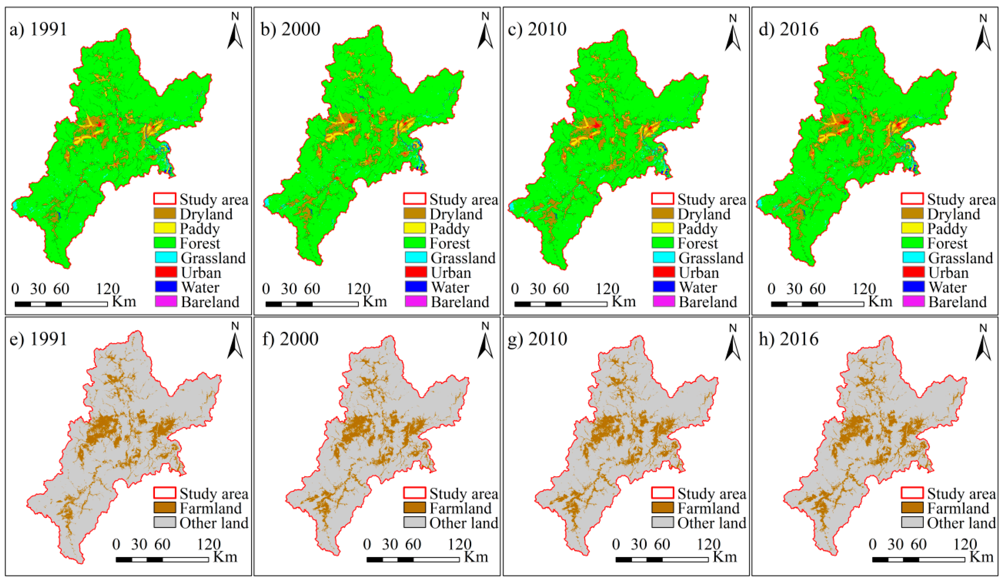
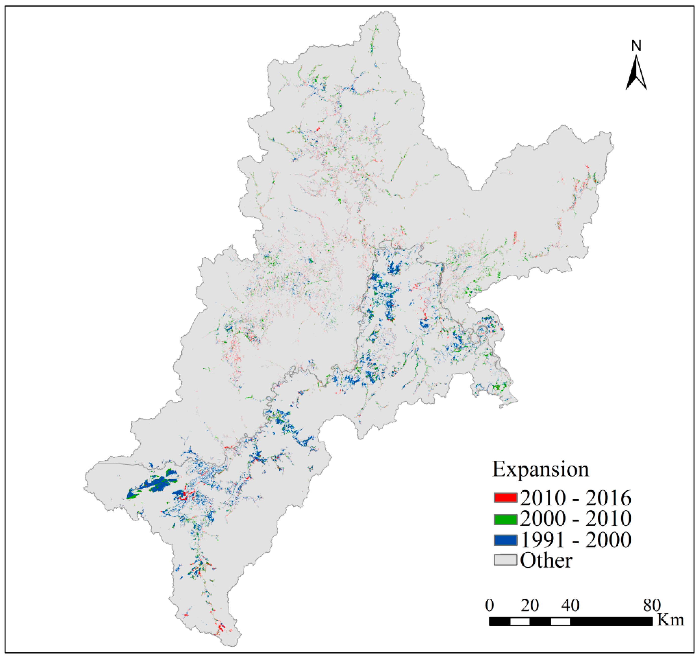
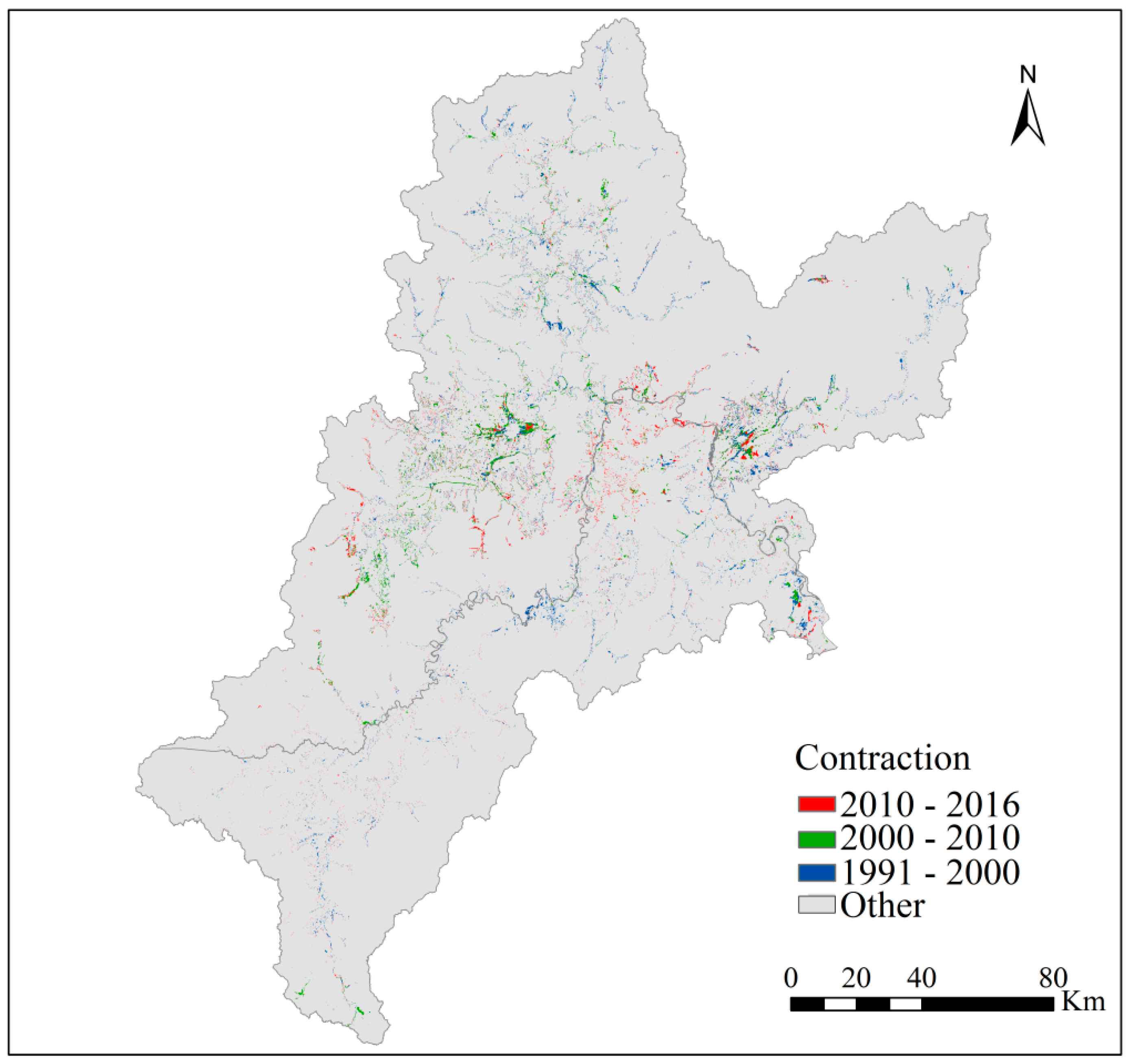
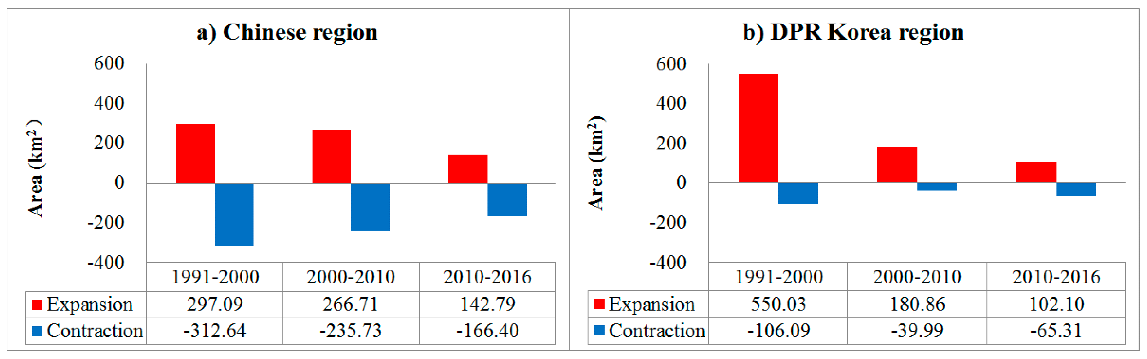
3.2. Spatiotemporal Farmland Changes

The data explored by the study reveal that expansions and contractions in farmland area co-occurred across the study region throughout different time periods (Figure 5, Figure 6 and Figure 7). Figure 5 and Figure 6 show the distributions of expansion and contraction in farmland, respectively.

Changes within DPR Korea and Chinese regions were characterized by large differences throughout these periods, and we note that farmland expansions within the former region were stronger than in the latter during the whole study period. Similarly, contractions in farmland area within China have been more marked than those in the DPR Korea TRB region throughout the time period of this study. Farmland expansions within the DPR Korea region of the TRB have mainly been at the expense of forested land, especially between 1991 and 2000 (Figure 5), while contractions (Figure 6) within China mainly occurred at sites adjacent to urban regions with low elevation; these phenomena can be characterized as farmland contractions due to urban expansion.

Results show that expansion areas within China between 1991 and 2000 and between 2010 and 2016 were smaller than areas of contraction. In contrast, farmland expansion areas between 2000 and 2010 were greater than contractions; as a whole, farmland across the Chinese region decreased between 1991 and 2000 and between 2010 and 2016, by −15.55 km² (−1.73 km²/year) and −23.61 km² (−3.94 km²/year), respectively, while an expansion area of 297.09 km² and a contraction area of −312.64 km² was seen between 1991 and 2000. An expansion area of 142.79 km² and a contraction area of −166.40 km² were seen between 2010 and 2016, respectively (Figure 7a); in contrast, this area increased by 30.98 km² (3.10 km²/year) between 2000 and 2010.

Farmland expansions within the DPR Korea region of the study area were clearer than concomitant contractions; these changes were widespread over all three time periods. Indeed, between 1991 and 2000, this region experienced intense farmland expansions, which were more significant than at other times (i.e., between 2000 and 2010, and 2010 and 2016), with expansions of 550.03 km² (61.14 km²/year) and contractions of −106.09 km² (17.68 km²/year). Between 2000 and 2010 and between 2010 and 2016, farmland expansions were also greater than contractions; this LULC type was increased by 140.87 km² (14.09 km²/year) with 180.86 km² of expansion area and −39.99 km² of contraction area between 2000 and 2010. A similar increase of 36.79 km² (6.13 km²/year) corresponds to an expansion area of 102.10 km² and a contraction of −65.31 km² between 2010 and 2016 (Figure 7b). The area of farmland within the DPR Korea region of the study area increased over all three time periods.

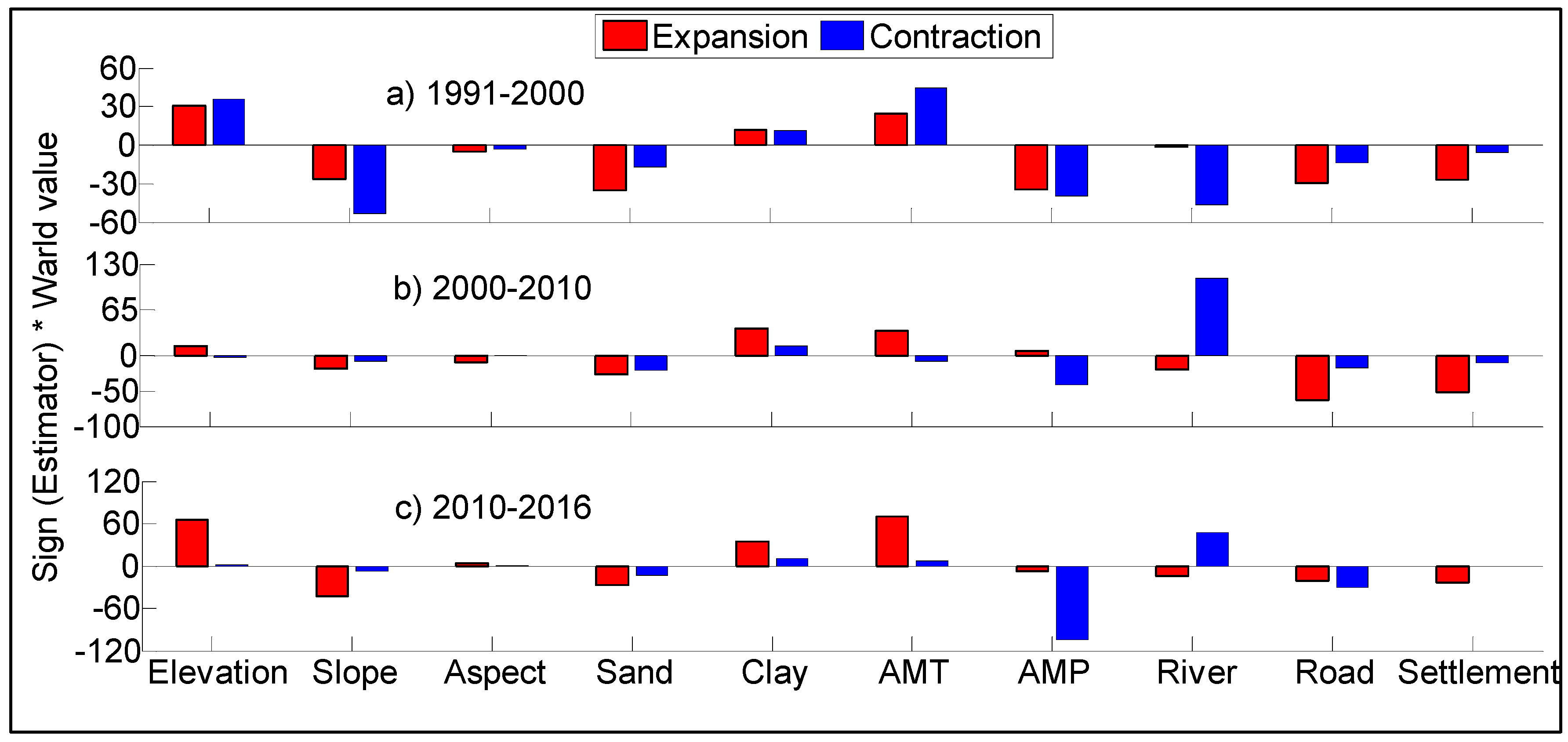
3.3. Factors Driving Farmland Changes

In order to determine the factors driving farmland expansions and contractions within Chinese and DPR Korea region of TRB, 12 LR models were estimated from the change maps for the period between 1991 and 2000, between 2000 and 2010, and between 2000 and 2016, respectively.

3.3.1. Factors Driving Farmland Expansion and Contraction within the Chinese TRB region

The data presented in

Table 4. Model estimates for farmland expansion driving forces across the Chinese region of the Tumen/Tuman River Basin (TRB).

Variables	Between 1991 and 2000		Between 2000 and 2010		Between 2010 and 2016
	Estimator	Wald	Estimator	Wald	Estimator	Wald
Elevation	1.864 ***	61.998	−0.919 **	6.953	0.642 **	10.177
Slope	−0.725 ***	112.465	−0.713 ***	108.083	−1.033 ***	151.483
Aspect	−0.008	0.018	−0.259 ***	17.711	−0.014	0.045
Soil sand content	−0.576 ***	30.202	−0.789 ***	58.415	−0.435 ***	17.139
Soil clay content	−0.063	0.391	−0.445 ***	20.233	0.095	0.737
AMT	2.845 ***	126.867	0.914 **	11.970	1.647 ***	56.255
AMP	−0.408 **	11.974	0.825 ***	24.092	−0.500 ***	27.042
River dist.	−0.364 **	10.864	−0.278 *	6.138	−0.179	2.240
Road dist.	−0.396 **	11.122	−0.360 **	9.761	−0.404 **	10.271
Settlement dist.	−0.331 ***	13.773	−0.611 ***	48.719	−0.562 ***	34.083
Constant	−0.330 ***	23.478	−0.240 ***	13.636	−0.373 ***	26.937
N	999		997		998
Overall PCP	80.9		80.4		84.4
AUC	0.811		0.877		0.902
Nagelkerke R2	0.561		0.540		0.611

Abbreviations: *, significant at p < 0.05; **, significant at p < 0.01; ***, significant at p < 0.001; N, number of points in one code.

summarize the results from the three driving force models for farmland expansions within the Chinese TRB region. Farmland expansions in this region were all significantly influenced by seven variables over all three time periods, specifically elevation, slope, and soil sand content, AMT and AMP, as well as distances to roads and settlements. We show that these variables were important driving factors of farmland expansions within the Chinese TRB region between 1991 and 2016. Temperature was positively related to farmland expansions across all three time periods, while slope, soil sand content, and distance to roads and settlements exerted negative effects in all cases. We also showed that elevation exerted a positive effect on expansion between 1991 and 2000 and between 2010 and 2016, but had a negative effect between 2000 and 2010. The positive effects of temperature on farmland expansion meant that farmland has preferentially expanded in areas with relatively high AMT values. Negative effects on farmland expansion were also seen in the case of slope, soil sand content; distance to roads and settlements and have caused farmland land use to expand preferentially within gentler slope areas, in regions close to roads and settlements, as well as in areas with lower soil sand content values.

The data presented in

Table 5. Potential drivers of farmland expansions in the three LR models placed in order of importance.

Variables	Between 1991 and 2000	Between 2000 and 2010	Between 2010 and 2016
Elevation	3	9	7
Slope	2	1	1
Aspect	-	6	-
Soil sand content	4	2	5
Soil clay content	-	5	-
AMT	1	7	2
AMP	6	4	4
River dist.	8	10	-
Road dist.	7	8	6
Settlement dist.	5	3	3

reveal the order to relative importance for individual driving forces between different study periods. We showed that the slope and AMT across three periods were more important than all others. Slope were ranked second, first, and first during the first, second and third time periods, respectively. AMT were ranked first, seventh, and second during three periods, respectively.

The data presented in

Table 6. Model estimations for the driving forces underlying farmland contractions within the Chinese TRB region.

Variables	Between 1991 and 2000		Between 2000 and 2010		Between 2010 and 2016
	Estimator	Wald	Estimator	Wald	Estimator	Wald
Elevation	0.664 **	6.567	0.315	0.587	1.851 ***	78.977
Slope	−0.813 ***	119.845	−0.925 ***	134.417	−0.465 ***	52.724
Aspect	−0.216 **	0.594	0.171 *	6.450	−0.136 *	5.062
Soil sand	−0.666 ***	38.531	−0.721 ***	43.331	−0.397 ***	17.890
Soil clay	−0.125	1.085	−0.404 ***	13.637	0.067	0.406
AMT	1.912 ***	55.638	1.864 ***	33.934	3.282 ***	197.821
AMP	−0.224 *	5.028	0.403 *	4.398	−0.539 ***	37.058
River dist.	−0.180	2.414	−0.226	3.604	0.022	0.049
Road dist.	−0.317 **	8.515	−0.416 **	11.263	0.098	0.887
Settlement dist.	−0.517 ***	28.807	−0.614 ***	40.891	−0.254 **	10.786
Constant	−0.300 ***	18.820	−0.302 ***	18.003	−0.213 **	11.719
N	999		942		999
Overall PCP	81.7		81.7		78.8
AUC	0.891		0.898		0.868
Nagelkerke R2	0.580		0.597		0.524

Abbreviations: *, significant at p < 0.05; **, significant at p < 0.01; ***, significant at p < 0.001; N, number of points in one code.

summarize results from the three models for farmland contraction driving forces within the Chinese TRB region. Farmland contractions during the three periods considered here were simultaneously affected by slope, aspect, soil sand content, AMT, and AMP, and distance to settlements. We show that slope and soil sand content variables negatively influenced farmland contraction across the three periods; this result means that farmland contractions across this area mainly occurred in regions with lower soil sand content and slope values. AMT values throughout all three time periods exerted positive effects on farmland contraction; this means that farmland areas mainly contracted in areas that were characterized relatively high values of AMT. The positive and negative roles played by other driving forces and their potentially significant effects on farmland contraction were complex and varied throughout the different time periods.

The order of relative importance of individual driving forces also varies between different study periods (

Table 7. Farmland contraction drivers in order of importance for the three LR models.

Variables	Between 1991 and 2000	Between 2000 and 2010	Between 2010 and 2016
Elevation	6	-	2
Slope	1	1	3
Aspect	-	7	7
Soil sand content	3	2	5
Soil clay content	-	5	-
AMT	2	4	1
AMP	7	8	4
River dist.	-	-	-
Road dist.	5	6	-
Settlement dist.	4	3	6

). Our data show that both slope and AMT variables exerted more important influences than their counterparts on farmland contractions throughout all study periods. Slope were ranked as first, first, and third during three periods, respectively. AMT were ranked second, fourth, and first, respectively.

3.3.2. Factors Driving Farmland Expansion and Contraction within the DPR Korea TRB Region

Table 8. Model estimates of farmland expansions driving forces within the DPR Korea region of study area.

Variables	Between 1991 and 2000		Between 2000 and 2010		Between 2010 and 2016
	Estimator	Wald	Estimator	Wald	Estimator	Wald
Elevation	2.701 ***	30.809	2.314 ***	13.489	4.449 ***	65.161
Slope	−0.322 ***	26.383	−0.279 ***	17.797	−0.474 ***	42.743
Aspect	−0.128 *	5.073	−0.183 **	9.362	0.134 *	4.129
Soil sand content	−0.621 ***	35.170	−0.456 ***	26.558	−0.458 ***	27.229
Soil clay content	0.340 **	11.970	0.563 ***	39.266	0.495 ***	35.080
AMT	2.622 ***	24.729	3.405 ***	35.349	4.869 ***	70.559
AMP	−0.929 ***	34.725	0.633 *	6.790	−0.292 **	7.449
River Dist.	−0.077	0.968	−0.390 ***	19.894	−0.339 ***	13.795
Road Dist.	−0.374 ***	29.558	−0.586 ***	62.666	−0.381 ***	21.703
Settlement Dist.	−0.444 ***	26.996	−0.620 ***	51.702	−0.469 ***	23.962
Constant	−0.217 **	13.109	−0.196 ***	9.485	−0.195 **	7.379
N	996		909		796
Overall PCP	75.9		77.6		75.9
AUC	0.844		0.854		0.847
Nagelkerke R2	0.445		0.474		0.462

Abbreviations: *, significant at p < 0.05; **, significant at p < 0.01; ***, significant at p < 0.001; N, number of points in one code.

shows results from the three models for farmland expansions driving forces within the DPR Korea TRB region. All nine variables had significantly influenced farmland expansions within the DPR Korea TRB region over the three times periods; these variables included elevation, slope, aspect, soil sand and clay content, AMT and AMP, and distance to roads and settlements (Table 8). Elevation, soil clay content and temperature have all exerted positive effects on farmland expansions over our three study periods, while slope, soil sand content, and distance to roads and settlements were all negatively related to this change. The positive and negative roles of AMP and aspect on farmland expansions have also varied between different study periods. Our results show that farmland expansions throughout all study periods more likely occurred in areas with relatively high altitude values as well as soil clay content and temperature, especially within areas with relatively low slope values, soil sand content, and distance to rivers. Results also revealed that topographic, climatic, and distance variables were the most important spatial determinants of expansions across all time periods.

Our data also show that the order of relative importance of individual driving factors varied between different periods; between 1991 and 2000, for example, soil sand content, precipitation, and elevation variables were more important than others in terms of farmland expansion (

Table 9. Drivers of farmland expansion in our three LR models ranked in order of importance.

Variables	Between 1991 and 2000	Between 2000 and 2010	Between 2010 and 2016
Elevation	3	8	2
Slope	6	7	3
Aspect	8	9	10
Soil sand content	1	5	5
Soil clay content	8	3	4
AMT	7	4	1
AMP	2	10	9
River dist.	-	6	8
Road dist.	4	1	7
Settlement dist.	5	2	6

); these all exhibit values of the Wald statistic higher than 30. In contrast, distance to roads and settlement between 2000 and 2010 exerted the most important influences on farmland expansion, and AMT and elevation for between 2000 and 2010 were the most important influences on farmland expansion.

Table 10. Model estimations for the forces driving farmland contractions within DPR Korea TRB region.

Variables	Between 1991 and 2000		Between 2000 and 2010		Between 2010 and 2016
	Estimator	Wald	Estimator	Wald	Estimator	Wald
Elevation	1.360 ***	35.759	−1.730	1.672	0.707	1.632
Slope	−0.287 ***	53.529	−0.359 **	8.399	−0.208 **	7.646
Aspect	−0.112	2.913	−0.037	0.112	0.036	0.260
Soil sand content	−0.498 ***	16.763	−0.533 ***	20.040	−0.316 ***	13.602
Soil clay content	0.532 ***	11.311	0.436 ***	14.103	0.269 **	11.164
AMT	4.390 ***	44.845	−3.219 **	8.332	1.572 **	7.574
AMP	−0.481 ***	39.676	−3.558 ***	40.951	−1.396 ***	104.445
River Dist.	−0.362 ***	46.635	2.341 ***	110.538	0.675 ***	47.054
Road Dist.	−0.434 ***	13.873	−0.587 ***	17.590	−0.483 ***	30.036
Settlement Dist.	−0.399 ***	5.366	−0.513 **	9.875	−0.054	0.249
Constant	−0.201 ***	8.697	−0.302 *	5.908	−0.259 **	11.291
N	832		302		596
Overall PCP	77.1		85.1		78.7
AUC	0.841		0.911		0.872
Nagelkerke R2	0.459		0.629		0.527

Abbreviations: *, significant at p < 0.05; **, significant at p < 0.01; ***, significant at p < 0.001; N, number of points in one code.

shows the results from the three LR models for farmland contraction driving forces within the DPR Korea region of TRB. The results show that seven variables significantly influenced farmland contractions within the region throughout all three times periods, and they are slope, soil sand and clay content, AMT, AMP, distances to river and road. Among them, slope, soil sand content, AMP and distance to road exerted negative effects on farmland contractions over all time periods studied, but the soil clay content was positively related to this change across the three periods. These results mean that farmland contractions across this region have preferentially contracted in regions with lower slope, soil sand content, precipitation, and relatively high values of soil clay content during all three periods.

Table 11. Drivers of farmland contraction in our three LR models ranked in order of importance.

Variables	Between 1991 and 2000	Between 2000 and 2010	Between 2010 and 2016
Elevation	5	-	-
Slope	1	7	6
Aspect	-	-	-
Soil sand content	6	3	4
Soil clay content	8	5	5
AMT	3	8	7
AMP	4	2	1
River dist.	2	1	2
Road dist.	7	4	3
Settlement dist.	9	6	-

shows the order to relative importance for different driving forces on farmland contractions within DPR Korea TRB region between different study periods. We show that the precipitation and river distance variables were more important than all others across three periods. Especially, the importance order of distance to river variable between 1991 and 2000, between 2000 and 2010, and between 2010 and 2016 were second, first, and second, respectively.

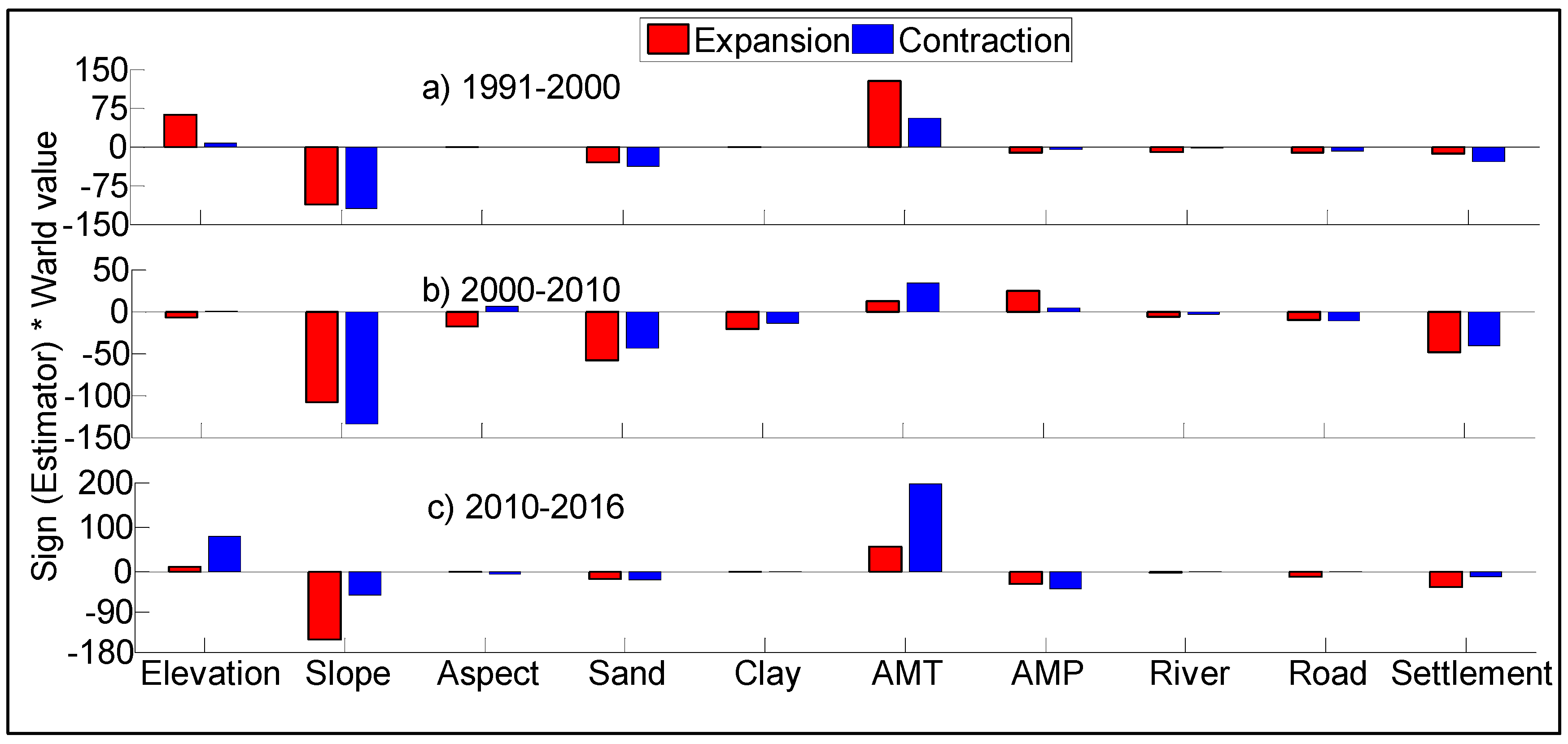
3.3.3. Comparisons of Driving Forces on Farmland Changes

A comparative analysis of the different factors leading to expansions and contractions in farmland respectively is beneficial for deeper understanding of the farmland change mechanisms within TRB. Figure 8 and Figure 9 show that the directions (i.e., positive or negative role) and the sizes (i.e., sign (estimator) × Wald value) on the relative importance of individual significant factors leading to farmland expansion and contraction between 1991 and 2000, between 2000 and 2010, and between 2010 and 2016 within Chinese (Figure 8) and DPR Korea (Figure 9) TRB regions, respectively.

The signs of the relative importance of the individual significant factors leading to farmland expansion and contraction within Chinese TRB region were the same during all three time periods (Figure 8a–c). It clearly shows that the slope, soil sand content, and distance to settlements had significant negative effects on farmland expansions and contractions during all of the periods studied. However, temperature exhibited significant positive effects on farmland expansions and contractions during three periods studied. Among all of the significant forces driving farmland changes, slope and temperature were the most important factors during all three time periods, and had negative and positive effects, respectively.

The signs of the relative importance of the different significant factors driving farmland expansions and contractions were also same between 1991 and 2000, and between 2010 and 2016 within the DPR Korea TRB region (Figure 9a,c). During these periods, AMT was a paramount positive factor on farmland changes. Between 2000 and 2010, the relative importance values of slope and soil sand content had same negative signs on farmland expansion and contraction, but soil clay content had same the positive signs, and while the signs of relative importance for other significant factors were opposite on farmland expansions and contractions (Figure 9b).

4. Discussion

4.1. Farmland Expansion and Contraction

We show that farmland area increased by 613.35 km² between 1991 and 2016 across the whole study region. Areas of farmland were increased by 428.35 km², 171.83 km², and 13.17 km², respectively, between 1991 and 2000, 2000 and 2010, and 2010 and 2016. At the same time, farmland change areas (i.e., expansion or contraction) varied with time periods and regions; the extraction and contraction of farmland in the Chinese part of the TRB simultaneously coexisted over the time periods studied. These extractions and contractions in farmland may be the result of human activities, including urbanization, cultural activities, and ecological restoration. Rapid urbanization and industrialization processes over recent decade across China have converted a growing area of cropland into housing or construction land [62]. Jilin Province proposed an ecological target in the late 1990s to remedy this, which led to the conversion of some cultivated land to woodland, grassland to farmland, and unused land to grassland, as well as population growth across the region; this led to an increase in urban residential and industrial land [63], mainly in farmland areas. These various urbanization, industrialization, and ecological construction activities across the Chinese TRB region appear to have been the main basis for farmland expansion and contraction.

Farmland expansions within the DPR Korea region of the TRB over the course of the three time periods were all larger than the areas of contraction. Data show that farmland expansion was very strong between 1991 and 2000; at this time, the average annual increase of farmland was 49.23 km²/year. It is clear that the DPR Korea region experienced considerable upland deforestation throughout the 1990s; 3490 km² of forested area (about 3.98% of the total area of this LULC) declined between 1990 and 2010, while major land use transitions occurred from closed canopy to open canopy forest, and from the latter to agricultural land [64]. In this earlier work, Pang et al. (2013) [64] studied Suan County in Hwanghae Province, DPR Korea, and showed that 20.72% of the closed canopy forest was lost over this time period, while agricultural lands expanded by 66.52% between 1979 and 2001. In contrast, during the two other time periods assessed here (i.e., between 2000 and 2010 and between 2010 and 2016), annual average increases in farmland area were 14.08 km²/year and 6.13 km²/year, respectively. It is noteworthy that since 2012, the government of DPR Korea has incorporated agroforestry as a national strategy for afforestation and livelihood development [64]; the decreasing rate of farmland expansion in the DPR Korea TRB area compared to the first period of this analysis may relate to these activities.

4.2. Driving Forces of Farmland Changes

The LR models used in this study proved to be effective for identifying the main driving forces of farmland changes within our study area regions. The two zones both exhibited Nagelkerke R² values greater than 0.44 in the case of all LR models, as well as AUC values greater than 0.811; thus all the LR models are credible. The farmland change driving forces results showed that this variation was affected by topographic, climatic, and distance factors, both spatially and temporally, and there were clear differences between them. The positive and negative directions of relative importance in the individual significant factors on farmland expansion and contraction within Chinese TRB region were all the same during all three time periods, and those at the DPR Korea side were also same, except for between 2000 and 2010 with slight contraction of areas in farmland, which may be related to characteristics of mountain areas and neighborhood land use from the limitation of available land area [65].

(1) Topographic factors: We show that topographic factors have proven to be the most important forces driving farmland changes within both different regions of the study area over all three time periods. Farmland expansions and contractions within the Chinese region have been simultaneously affected by slope, elevation, and aspect. Among of them, slope and elevation in both regions throughout all periods mostly played negative and positive roles on farmland changes, respectively. Previous studies have shown that both these key variables play important roles in determining land use in mountain areas [46,66]; this is in part because lower elevations and gentler slopes tend to be more suitable for human urbanization and agricultural activities than higher areas [65], because of land management issues. However, elevation on farmland changes had positive effects between 1991 and 2000, and between 2010 and 2016 across these regions. Areas of farmland across the TRB tend to be located in narrow valley regions with low mountain slopes; although these are convenient areas for human activities, they are nevertheless limited in abundance within the region. Expansions and contractions in farmland are therefore more likely to occur in marginal forested areas, and across farmland that exhibit gentle slopes via deforestation and cultivation activities. This result is consistent with the results on cropland expansion and contraction in the Koshi River Basin of the Central Himalayas, Nepal of Paudel et al. (2016) [15]. The analysis reveals that absolute values of relative importance (Wald value) for slopes in controlling both farmland expansions and contractions across the two different regions of the TRB have been greater than those for elevation during our different study periods. The slope variable in Chinese regions of the TBR has therefore been of paramount importance in driving farmland changes, while the roles of elevation and slope were similar with opposed sign effects on farmland changes within the DPR Korea region.

(2) Soil factors: The farmland expansion and contraction within Chinese area were mainly influenced by the negative effect of soil sand content during the studied periods. In the DPR Korea region of the study area, soil sand and clay content were both significant factors controlling farmland expansion and contraction during the three time periods, which also exhibited both positive and negative effects on farmland expansion and contraction, respectively. The negative effect of soil sand content on farmland expansion within the Chinese TRB region might be due to agricultural activities in adjacent areas where the soil sand content is lower; similarly, the negative effects of soil sand content on farmland contraction might also be due to human urbanization in central farmland zones. While, in the DPR Korea region of the study area, lands with lower soil sand content and higher clay content are more likely to be cultivated even if they are mountainous, and farmland contractions might also occur in farmland areas with lower soil sand content and higher clay content by urbanizations, because of the limitation on suitable regions for human activities in this area. This illustrated that farmland land with higher soil sand content and lower soil clay content was easily translated into other land, this is in concurrence with a study on dynamic mechanisms of farmland abandonment in Jiangxi Province, China, by Xie et al. (2014) [10]. While opposite land was favorable for agricultural activity and production in the study area.

(3) Climatic factors: In terms of climatic factors, we show that changes to farmland across our study region were also affected by AMT and AMP across all three time periods. The relationships between AMT and farmland expansion and contraction have mostly exerted a positive effect across both regions and different time periods. The examined study region is characterized by a typical temperate monsoonal climate and experiences average temperatures between 2 °C and 6 °C [30], the rising temperatures in this area become more favorable for crop growth; the positive effects of AMT on farmland expansions in different regions might therefore be due to the fact that areas where temperature is rising tend to be more favorable for agricultural production. These positive effects of temperature on farmland expansions also appeared in existing study [16] in Panxi mountainous region, China. At the same time, the positive effects of AMT on farmland contractions might also be due to urbanization and reforestation, as these regions are also favorable for human activities and plant growth [16].

Our data show that the relationship between precipitation and farmland changes can be both positive and negative, corroborating earlier work [15]. Results show that AMP mostly exerted a negative influence on both farmland expansions and contractions across two different regions of the study area. Our study area falls within a humid-to-semi-humid region [29] that has relatively high soil moisture content, especially in the growing period for major crops such as rice, corn, and soybean; approximately 70% of the total rainfall occurs between June and September. Excessive soil moisture conditions can decrease the yields of these major crops. This region is also close to the East Sea of Korea and is therefore climatically influenced by the ocean. The clearly negative effects of farmland expansions in different regions mean that area where precipitation has reduced over time tends to be more favorable for agricultural production. The negative effects of precipitation on farmland contraction mean that farmland contractions in different regions may appear by their transformation into other land use types, such as settlements in areas where precipitation has increased, because relatively high moisture is not favorable for agricultural production in our study area. The other effects of precipitation on farmland changes have proven to be more complex and hard to understand than first thought.

The results of this analysis clearly imply that the positive role of temperature on TRB farmland changes was larger over the whole time period of analysis compared to the negative role of precipitation.

(4) Distance factors: Numerous previous studies have shown that distance factors have been key variables in terms of driving farmland changes [3,10,15,17]. The results of this analysis show that distance factors within both different regions of the study area mostly exert a negative influence on farmland expansions and contractions throughout three time periods. The roles of distance to road and settlement on farmland expansions were most significant in the Chinese TRB region, while all distance factors in DPR Korea TRB region were significant for farmland changes. An existing study [15] to address farmland changes in the Koshi River Basin (KRB) of the Central Himalayas, Nepal showed that the distance factors (i.e., distances to rivers, settlements, and roads) have mostly positive relationships with farmland expansion and contraction. This is not consistent with our results. Farmland areas in the KRB [15] were widely distributed across most of the basin area; however, in our study area, they were distributed in limited parts only. The favorable area for human activities was also limited in our study area by relative higher and steeper slopes. These findings mean that farmland expansion and contraction within the Chinese TRB region are likely to appear in areas adjacent to roads and settlements during all three time periods studied; while the farmland changes within DPR Korea TRB region are likely to occur in areas adjacent to rivers, roads, and settlements. These extractions and contractions in farmland were affected by urbanization, cultural activities, and ecological restoration.

5. Conclusions

The analytical results presented here reveal large differences in farmland changes within both different regions of the TRB between 1991 and 2000, 2000 and 2010, and 2010 and 2016. Data show that the farmland area within the DPR Korea TRB region has mainly increased over time; expansion of farmland has been greater than its contraction throughout this analysis. Farmland contractions within the Chinese TRB region have been more marked than those seen in DPR Korea TRB region; areas of farmland decreased between 1991 and 2000 and between 2010 and 2016, because of an overall lower expansion rate compared to the contracted areas. In contrast, the farmland area between 2000 and 2010 increased a little, as the opposite relationship was true. LR results also reveal that topographic (i.e., slope and elevation), soil (soil sand content and clay content), climactic (i.e., AMT and AMP) and distance (i.e., distances to rivers, roads, and settlements) factors have significantly influenced farmland changes across the different regions of the study area over time. Among them, slope and temperature in Chinese area have been of paramount importance, with negative and positive effects on farmland changes over different study periods, respectively; on the other hand, the temperature in DPR Korea TRB region have also played a paramount positive role on farmland expansion, and AMP have played a paramount positive role on farmland contraction. Expansions in farmland area were widespread within boundary regions between farmland and forest over the three time periods evaluated here, because of difficulties with farming and higher cultivation costs encountered in areas with relatively higher elevation and steeper slope. Farmland contractions are more likely to have occurred in agricultural areas adjacent to settlements, as well as in boundary regions between farmland and forest, because of national urbanization and afforestation policies. It is clearly shown that most of the significant driving factors of farmland changes were exposed to the same directions on farmland expansions and contractions in different periods studied, due to mountainous topographic characteristics, although their relative importance on farmland changes took effect at different rates. The trends from our results may also be appearing in other cross-border regions with similar geographic and socioeconomic conditions.

The results of this analysis support the conclusion that farmland expansions and contractions in the study area were mainly due to deforestation (expansion), as well as urbanization, industrialization, and afforestation activities (contraction). In addition to the driving forces discussed in this analysis, it is clear that additional factors such as land use policies, management, GDP, labor migration, and natural hazards will also play an important role in farmland changes. Data limitations, however, did not allow exploring these variables. In order to quantitatively estimate the contributions of these additional factors to farmland changes, more data collection and the development of more appropriate analytical approaches will be required.

References

1. Zhang, Y.L.; Nie, Y.; Lv, X.F. Chinese literature analysis on land use research in China. Progr. Sci. 2008, 27, 1–11. [Google Scholar]
2. Liu, C.; Xu, Y.; Sun, P.; Huang, A.; Zheng, W. Land use change and its driving forces toward mutual conversion in Zhangjiakou City, a farming-pastoral ecotone in Northern China. Environ. Monit. Assess. 2017, 189, 1–20. [Google Scholar] [CrossRef] [PubMed]
3. Huang, Q.; Cai, Y.; Peng, J. Modeling the spatial pattern of farmland using GIS and multiple logistic regression: A case study of Maotiao River Basin, Guizhou Province, China. Environ. Model. Assess. 2007, 12, 55–61. [Google Scholar] [CrossRef]
4. Du, X.; Jin, X.; Yang, X.; Yang, X.; Zhou, Y. Spatial Pattern of land use change and its driving force in Jiangsu Province. Int. J. Environ. Res. Public Health 2014, 11, 3215–3232. [Google Scholar] [CrossRef] [PubMed]
5. Gong, J.; Liu, Y.; Xia, B. Spatial heterogeneity of urban land-cover landscape in Guangzhou from 1990 to 2005. J. Geogr. Sci. 2009, 19, 213–224. [Google Scholar] [CrossRef]
6. Deng, X.Z.; Zhao, C.H.; Yan, H.M. Systematic modeling of impacts of land use and land cover changes on regional climate: A Review. Adv. Meteorol. 2013, 2013, 1–11. [Google Scholar] [CrossRef]
7. Foley, J.A.; DeFries, R.; Asner, G.P.; Barford, C.; Bonan, G.; Carpenter, S.R.; Chapin, F.S.; Coe, M.T.; Daily, G.C.; Gibbs, H.K.; et al. Global consequences of land use. Science 2005, 309, 570–574. [Google Scholar] [CrossRef] [PubMed]
8. Wang, G.; Liu, Y.; Li, Y.; Chen, Y. Dynamic trends and driving forces of land use intensification of cultivated land in China. J. Geogr. Sci. 2015, 25, 45–57. [Google Scholar] [CrossRef]
9. Dong, J.; Liu, J.; Yan, H.; Tao, F.; Kuang, W. Spatio-temporal pattern and rationality of land reclamation and cropland abandonment in mid-eastern Inner Mongolia of China in 1990–2005. Environ. Monit. Assess. 2011, 179, 137–153. [Google Scholar] [CrossRef] [PubMed]
10. Xie, H.; Wang, P.; Yao, G. Exploring the dynamic mechanisms of farmland abandonment based on a spatially explicit economic model for environmental sustainability: A case study in Jiangxi Province, China. Sustainability 2014, 6, 1260–1282. [Google Scholar] [CrossRef]
11. Quan, B.; Chen, J.F.; Qiu, H.L.; Romkens, M.J.M.; Yang, X.Q.; Liang, S.F.; Li, B.C. Spatial-temporal pattern and driving forces of land use changes in Xiamen. Soil Sci. Soc. China 2006, 4, 477–488. [Google Scholar] [CrossRef]
12. Lei, Z.; Bingfang, W.; Liang, Z.; Peng, W. Patterns and driving forces of cropland changes in the Three Gorges Area, China. Reg. Environ. Chang. 2012, 12, 765–776. [Google Scholar] [CrossRef]
13. Dong, J.; Xiao, X.; Kou, W.; Qin, Y.; Zhang, G.; Li, L.; Jin, C.; Zhou, Y.; Wang, J.; Biradar, C.; et al. Tracking the dynamics of paddy rice planting area in 1986–2010 through time series Landsat images and phenology-based algorithms. Remote Sens. Environ. 2015, 160, 99–113. [Google Scholar] [CrossRef] [Green Version]
14. Liu, J.; Kuang, W.; Zhang, Z.; Xu, X.; Qin, Y.; Ning, J.; Zhou, W.; Zhang, S.; Li, R.; Yan, C.; et al. Spatiotemporal characteristics, patterns, and causes of land-use changes in China since the late 1980s. J. Geogr. Sci. 2014, 24, 195–210. [Google Scholar] [CrossRef]
15. Paudel, B.; Gao, J.; Zhang, Y.; Wu, X.; Li, S.; Yan, J. Changes in cropland status and their driving factors in the Koshi River Basin of the Central Himalayas, Nepal. Sustainability 2016, 8, 933. [Google Scholar] [CrossRef]
16. Peng, L.; Chen, T.; Liu, S. Spatiotemporal dynamics and drivers of farmland changes in Panxi Mountainous Region, China. Sustainability 2016, 8, 1209. [Google Scholar] [CrossRef]
17. Chen, Z.; Lu, C.; Fan, L. Farmland changes and the driving forces in Yucheng, North China Plain. J. Geogr. Sci. 2012, 22, 563–573. [Google Scholar] [CrossRef] [Green Version]
18. Pijanowski, B.C.; Brown, D.G.; Shellito, B.A.; Manik, G.A. Using neural networks and GIS to forecast land use changes: A Land Transformation Model. Comput. Environ. Urban Syst. 2002, 26, 553–575. [Google Scholar] [CrossRef]
19. Zewdie, M.; Worku, H.; Bantider, A. Temporal dynamics of the driving factors of urban landscape change of addis ababa during the past three decades. Environ. Manag. 2018, 61, 132–146. [Google Scholar] [CrossRef] [PubMed]
20. Long, H.; Tang, G.; Li, X.; Heilig, G.K. Socio-economic driving forces of land-use change in Kunshan, the Yangtze River Delta economic area of China. J. Environ. Manag. 2007, 83, 351–364. [Google Scholar] [CrossRef] [PubMed]
21. Li, X.; Zhou, W.; Ouyang, Z. Forty years of urban expansion in Beijing: What is the relative importance of physical, socioeconomic, and neighborhood factors? Appl. Geogr. 2013, 38, 1–10. [Google Scholar] [CrossRef] [Green Version]
22. Dong, G.; Xu, E.; Zhang, H. Spatiotemporal variation of driving forces for settlement expansion in different types of Counties. Sustainability 2016, 8, 39. [Google Scholar] [CrossRef]
23. Ellis, E.A.; Baerenklau, K.A.; Marcos-Martínez, R.; Chávez, E. Land use/land cover change dynamics and drivers in a low-grade marginal coffee growing region of Veracruz, Mexico. Agrofor. Syst. 2010, 80, 61–84. [Google Scholar] [CrossRef] [Green Version]
24. Najmuddin, O.; Deng, X.; Bhattacharya, R. The Dynamics of Land Use/Cover and the statistical assessment of cropland change drivers in the Kabul River Basin, Afghanistan. Sustainability 2018, 10, 423. [Google Scholar] [CrossRef]
25. Yu, B.; Song, W.; Lang, Y. Spatial patterns and driving forces of greenhouse land change in Shouguang City, China. Sustainability 2017, 9, 359. [Google Scholar] [CrossRef]
26. Nan, Y.; Ji, G.; Dong, Y.H.; Ni, X.J. Study of Land use/cover dynamic change in Tumen River across national border region during the last 30 years. J. Natl. Sci. Hunan Norm. Univ. 2012, 35, 82–89. [Google Scholar]
27. National action plan to combat desertification land degradation in Democratic People’s Republic of Korea (2006–2010). Available online: https://knowledge.unccd.int/sites/default/files/naps/democratic_people%60s_republic_of_korea-eng2006.pdf (accessed on 11 April 2018).
28. Gao, W.Y.; Zhu, C.F.; Wang, Y.S. Analysis on characteristic of hydrology and meteorology for Tumen river Basin. Jilin Water Resour. 2000, 12, 22–24. [Google Scholar]
29. Kang, C.; Zhang, Y.; Wang, Z.; Liu, L.; Zhang, H.; Jo, Y. The Driving force analysis of ndvi dynamics in the trans-boundary Tumen River Basin between 2000 and 2015. Sustainability 2017, 9, 2350. [Google Scholar] [CrossRef]
30. Zheng, X.J.; Sun, P.; Zhu, W.H.; Xu, Z.; Fu, J.; Man, W.D.; Li, H.L.; Zhang, J.; Qin, L. Landscape dynamics and driving forces of wetlands in the Tumen River Basin of China over the past 50 years. Landsc. Ecol. Eng. 2017, 13, 237–250. [Google Scholar] [CrossRef]
31. Chen, J.; Chen, J.; Liao, A.P.; Cao, X.; Chen, L.J.; Chen, X.H.; He, C.Y.; Han, G.; Peng, S.; Lu, M.; et al. Global land cover mapping at 30m resolution: A POK-based operational approach. SPRS J. Photog. 2014, 103, 1–21. [Google Scholar] [CrossRef]
32. Losiri, C.; Nagai, M.; Ninsawat, S.; Shrestha, R. Modeling urban expansion in Bangkok Metropolitan Region using demographic-economic data through cellular automata-markov chain and multi-layer perceptron-markov chain models. Sustainability 2016, 8, 686. [Google Scholar] [CrossRef]
33. Luo, Z.; Yu, S. Spatiotemporal variability of land surface phenology in China from 2001–2014. Remote Sen. 2017, 9, 65. [Google Scholar] [CrossRef]
34. Tang, Z.; Ma, J.; Peng, H.; Wang, S.; Wei, J. Spatiotemporal changes of vegetation and their responses to temperature and precipitation in upper Shiyang river basin. Adv. Space Res. 2016, 60, 969–979. [Google Scholar] [CrossRef]
35. Poursanidis, D.; Chrysoulakis, N.; Mitraka, Z. Landsat 8 vs. Landsat 5: A comparison based on urban and peri-urban land cover mapping. Int. J. Appl. Earth Obs. Geoinf. 2015, 35, 259–269. [Google Scholar] [CrossRef]
36. Devadasa, R.; Denham, R.J.; Pringle, A. Support vector machine classification of object-based data for crop mapping, using multi-temporal Landsat imagery. Int. Arch. Photogramm. Remote Sens. Spat. Inf. Sci. ISPRS Congr. 2012, 25, 185–190. [Google Scholar] [CrossRef]
37. Cortes, C.; Vapnik, V. Support-vector networks. Mach. Learn. 1995, 20, 273–297. [Google Scholar] [CrossRef] [Green Version]
38. Gao, Z.; Liu, X. Support Vector Machine and Object-oriented Classification for urban impervious surface extraction from satellite imagery. In Proceedings of the 2014 the Third International Conference on Agro-Geoinformatics, Beijing, China, 11–14 August 2014; pp. 1–5. [Google Scholar]
39. Luis Vega, L.; Hirata, Y.; Ventura Santos, L.; Serrudo Torobeo, N. Natural forest mapping in the Andes (Peru): A comparison of the performance of machine-learning algorithms. Remote Sens. 2018, 10, 782. [Google Scholar] [CrossRef]
40. Chatziantoniou, A.; Psomiadis, E.; Petropoulos, G. Co-Orbital Sentinel 1 and 2 for LULC mapping with emphasis on wetlands in a mediterranean setting based on machine learning. Remote Sens. 2017, 9, 1259. [Google Scholar] [CrossRef]
41. Rimal, B.; Zhang, L.; Keshtkar, H.; Haack, B.; Rijal, S.; Zhang, P. Land Use/Land Cover dynamics and modeling of urban land expansion by the integration of Cellular Automata and Markov Chain. ISPRS Int. J. Geo-Inf. 2018, 7, 154. [Google Scholar] [CrossRef]
42. Kavzoglu, T.; Colkesen, I. A kernel functions analysis for support vector machines for land cover classification. Int. J. Appl. Observ. Geoinf. 2009, 11, 352–359. [Google Scholar] [CrossRef]
43. Xue, W.; Jungang, G.; Yili, Z.; Linshan, L.; Zhilong, Z.; Paudel, B. Land cover status in the Koshi River Basin, Central Himalayas. J. Resour. Ecol. 2017, 8, 10–19. [Google Scholar] [CrossRef]
44. Alqurashi, A.; Kumar, L.; Al-Ghamdi, K. Spatiotemporal modeling of urban growth predictions based on driving force factors in Five Saudi Arabian Cities. ISPRS Int. J. Geo-Inf. 2016, 5, 139. [Google Scholar] [CrossRef]
45. Li, X.M.; Wang, Y.; Li, J.F.; Lei, B. Physical and socioeconomic driving forces of Land-use and Land-cover changes: A case study of Wuhan City, China. Discret. Dyn. Nat. Soc. 2016, 2016, 1–11. [Google Scholar] [CrossRef]
46. Bender, O.; Boehmer, H.J.; Jens, D.; Schumacher, K.P. Using GIS to analyse long-term cultural landscape change in Southern Germany. Landsc. Urban Plan. 2005, 70, 111–125. [Google Scholar] [CrossRef] [Green Version]
47. Gellrich, M.; Baur, P.; Koch, B.; Zimmermann, N.E. Agricultural land abandonment and natural forest re-growth in the Swiss mountains: A spatially explicit economic analysis. Agric. Ecosyst. Environ. 2007, 118, 93–108. [Google Scholar] [CrossRef]
48. Piedallu, C.; Gégout, J. Efficient assessment of topographic solar radiation to improve plant distribution models. Agric. For. Meteorol 2008, 148, 1696–1706. [Google Scholar] [CrossRef]
49. Karamage, F.; Zhang, C.; Ndayisaba, F.; Shao, H.; Kayiranga, A.; Fang, X.; Nahayo, L.; Muhire Nyesheja, E.; Tian, G. Extent of cropland and related soil erosion risk in Rwanda. Sustainability 2016, 8, 609. [Google Scholar] [CrossRef]
50. Bakker, M.M.; Govers, G.; Kosmas, C.; Vanacker, V.; Oost, K.V.; Rounsevell, M. Soil erosion as a driver of land-use change. Agric. Ecosyst. Environ. 2005, 105, 467–481. [Google Scholar] [CrossRef]
51. Wang, H.; Kong, X.; Zhang, B. The simulation of LUCC based on Logistic-CA-Markov model in Qilian Mountain area, China. Sci. Cold Arid Reg. 2016, 4, 350–358. [Google Scholar]
52. Gao, J.; Zhang, Y.; Liu, L.; Wang, Z. Climate change as the major driver of alpine grasslands expansion and contraction: A case study in the Mt. Qomolangma (Everest) National Nature Preserve, southern Tibetan Plateau. Quat. Int. 2014, 336, 108–116. [Google Scholar] [CrossRef]
53. Cheng, J.; Masser, I. Urban growth pattern modeling: A case study of Wuhan city, PR China. Landsc. Urban Plan 2003, 62, 199–217. [Google Scholar] [CrossRef]
54. Kleinbaum, D.G.; Klein, M. Logistic Regression; Springer: New York, NY, USA, 2002. [Google Scholar]
55. Menard Six Approaches to Calculating Standardized Logistic Regression Coefficients. Am. Stat. 2004, 3, 218–223.
56. Hamdy, O.; Zhao, S.A.; Salheen, M.; Eid, Y.Y. Analyses the driving forces for urban growth by using IDRISI®Selva Models Abouelreesh—Aswan as a Case Study. Int. J. Eng. Technol. 2017, 9, 226–232. [Google Scholar] [CrossRef]
57. Hu, Y.; Zheng, Y.; Zheng, X. Simulation of land-use scenarios for Beijing using CLUE-S and Markov composite models. Chin. Geogr. Sci. 2013, 23, 92–100. [Google Scholar] [CrossRef]
58. Jokar Arsanjani, J.; Helbich, M.; Kainz, W.; Darvishi Boloorani, A. Integration of logistic regression, Markov chain and cellular automata models to simulate urban expansion. Int. J. Appl. Earth Obs. 2013, 21, 265–275. [Google Scholar] [CrossRef]
59. Adhikari, S.; Fik, T.; Dwivedi, P. Proximate causes of Land-Use and Land-Cover Change in Bannerghatta National Park: A spatial statistical model. Forests 2017, 8, 342. [Google Scholar] [CrossRef]
60. Wagner, P.D.; Waske, B. Importance of spatially distributed hydrologic variables for land use change modeling. Environ. Model. Softw. 2016, 83, 245–254. [Google Scholar] [CrossRef]
61. Foody, G.M. Status of land cover classification accuracy assessment. Environ. MOdel. Softw. 2002, 80, 185–201. [Google Scholar] [CrossRef]
62. Ding, M.; Chen, Q.; Xiao, X.; Xin, L.; Zhang, G.; Li, L. Variation in Cropping Intensity in Northern China from 1982 to 2012 Based on GIMMS-NDVI data. Sustainability 2016, 8, 1123. [Google Scholar] [CrossRef]
63. Zhan, C.X.; Liu, Z.M.; Zeng, N. Using remote sensing and GIS to investigate land use dynamic change in Western Plain oF Jilin Province. Int. Arch. Photogramm. Remote Sens. Spat. Inf. Sci. 2008, 37, 1685–1689. [Google Scholar]
64. Pang, C.; Yu, H.; He, J.; Xu, J. Deforestation and changes in landscape patterns from 1979 to 2006 in Suan County, DPR Korea. Forests 2013, 4, 968–983. [Google Scholar] [CrossRef]
65. Kim, I.; Le, Q.; Park, S.; Tenhunen, J.; Koellner, T. Driving forces in archetypical land-use changes in a mountainous watershed in East Asia. Land 2014, 3, 957–980. [Google Scholar] [CrossRef]
66. Mottet, A.; Ladet, S.; Coqué, N.; Gibon, A. Agricultural land-use change and its drivers in mountain landscapes: A case study in the Pyrenees. Agric. Ecol. Environ. 2006, 114, 296–310. [Google Scholar] [CrossRef]
Figure 1. Location of study area and the distribution examples of reference data (a) for 2010 land cover classification and farmland status (b,c).
Ijgi 07 00352 g001
Figure 2. Framework overview of this study. Note: SS indicates spatial sampling; ZS is Z-score standardization; MLT is multicollinearity test; LR is logistic regression model.
Ijgi 07 00352 g002
Figure 3. Potential 2010 factors considered for the study area.
Ijgi 07 00352 g003
Figure 4. The results of land cover (ad) and farmland classification (eh) for different years.
Ijgi 07 00352 g004
Figure 5. Spatial pattern of farmland expansion across different regions over the three times.
Ijgi 07 00352 g005
Figure 6. Spatial pattern of farmland contraction across different regions over the three times.
Ijgi 07 00352 g006
Figure 7. Proportions (a,b) of farmland changes across different regions over the three time periods evaluated in this study.
Ijgi 07 00352 g007
Figure 8. Comparative analysis of the relative importance of different factors driving the farmland expansions and contractions within Chinese TRB region.
Ijgi 07 00352 g008
Figure 9. Comparative analysis of the relative importance of different factors driving the farmland expansions and contractions within the DPR Korea TRB region.
Ijgi 07 00352 g009