Interactive and Online Buffer-Overlay Analytics of Large-Scale Spatial Data


College of Electronic Science, National University of Defense Technology, Changsha 410073, China
*
Author to whom correspondence should be addressed.
ISPRS Int. J. Geo-Inf. 2019, 8(1), 21; https://0-doi-org.brum.beds.ac.uk/10.3390/ijgi8010021
Submission received: 2 December 2018
/
Revised: 1 January 2019
/
Accepted: 8 January 2019
/
Published: 10 January 2019
(This article belongs to the Special Issue GIS Software and Engineering for Big Data)
Abstract
:Buffer and overlay analysis are fundamental operations which are widely used in Geographic Information Systems (GIS) for resource allocation, land planning, and other relevant fields. Real-time buffer and overlay analysis for large-scale spatial data remains a challenging problem because the computational scales of conventional data-oriented methods expand rapidly with data volumes. In this paper, we present HiBO, a visualization-oriented buffer-overlay analysis model which is less sensitive to data volumes. In HiBO, the core task is to determine the value of pixels for display. Therefore, we introduce an efficient spatial-index-based buffer generation method and an effective set-transformation-based overlay optimization method. Moreover, we propose a fully optimized hybrid-parallel processing architecture to ensure the real-time capability of HiBO. Experiments on real-world datasets show that our approach is capable of handling ten-million-scale spatial data in real time. An online demonstration of HiBO is provided (http://www.higis.org.cn:8080/hibo).
1. Introduction
A buffer is defined as the zone with a certain width around a geometric geographic feature, according to a specified buffer distance, and an overlay creates a composite map by combining the geometry and attributes of multiple data layers [1]. Buffer and overlay analysis are two basic Geographic Information System (GIS) spatial operations for resource allocation, land planning, and many other relevant fields [2,3]. In practical applications, the two operations are usually combined to solve spatial decision problems; typically, the site selection problem [4]. In this paper, we use buffer-overlay analysis to represent the combined operation.
Buffer-overlay analysis is computationally intensive and time-consuming. Moreover, with the rapid development of surveying and mapping technology, the computational limitation becomes more prominent as greater volumes of large-scale spatial data is produced.
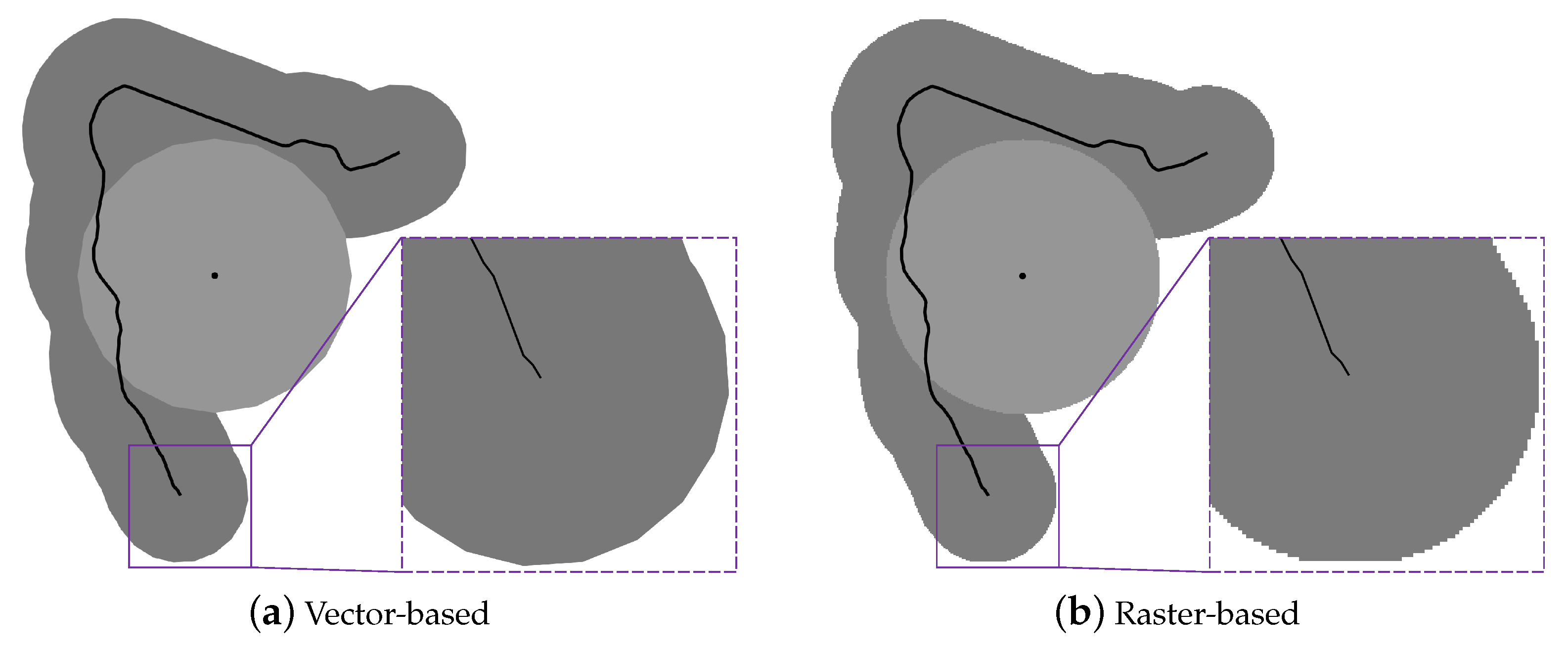
Buffer and overlay generation are the keys to buffer-overlay analysis. Several methods for solving generation problems have been proposed. These methods can be summarized into two categories, by the types of results they produce: Vector-based methods and raster-based methods. Vector-based methods use vector polygons to represent results, while raster-based methods use values of pixels in raster images to indicate result zones. Table 1 lists the advantages and disadvantages of the two types of methods. Due to their large storage space occupancy, raster-based methods are generally not applied to large-scale spatial data, and the related research mainly focuses on the calculation of raster buffers using a serial computing model [5,6]. For vector-based methods, the edge constraint triangulation method [7] and the buffer equation approximation strategy are widely used [8] in buffer generation; in addition, in order to deal with large-scale data, several parallel strategies have been proposed to solve the vector-based buffer and overlay generation problems [9,10,11,12,13,14,15,16,17]. However, the performance is still far from satisfactory as it is impossible to support real-time buffer-overlay analysis using the traditional methods, even when high-performance computing technologies are applied. For example, Shen [10] proposed a parallel vector buffer generation method, HPBM, based on Spark [18], and conducted an experiment on a high-performance cluster which compared HBPM to three optimized parallel methods and the popular GIS software programs (Table 2); as shown in the table, HBPM outperformed the other traditional data-oriented methods and is able to generate buffers for 597k linestring objects in around 3 min. As another example, Puri [16] presented a parallel GIS system, MPI-GIS, for polygon overlay processing of two GIS layers which employs R-tree for efficient indexing and identification of potentially intersecting sets of polygon objects; using MPI-GIS, the processing time of hundred-thousand-scale datasets is in the ten-second-level.
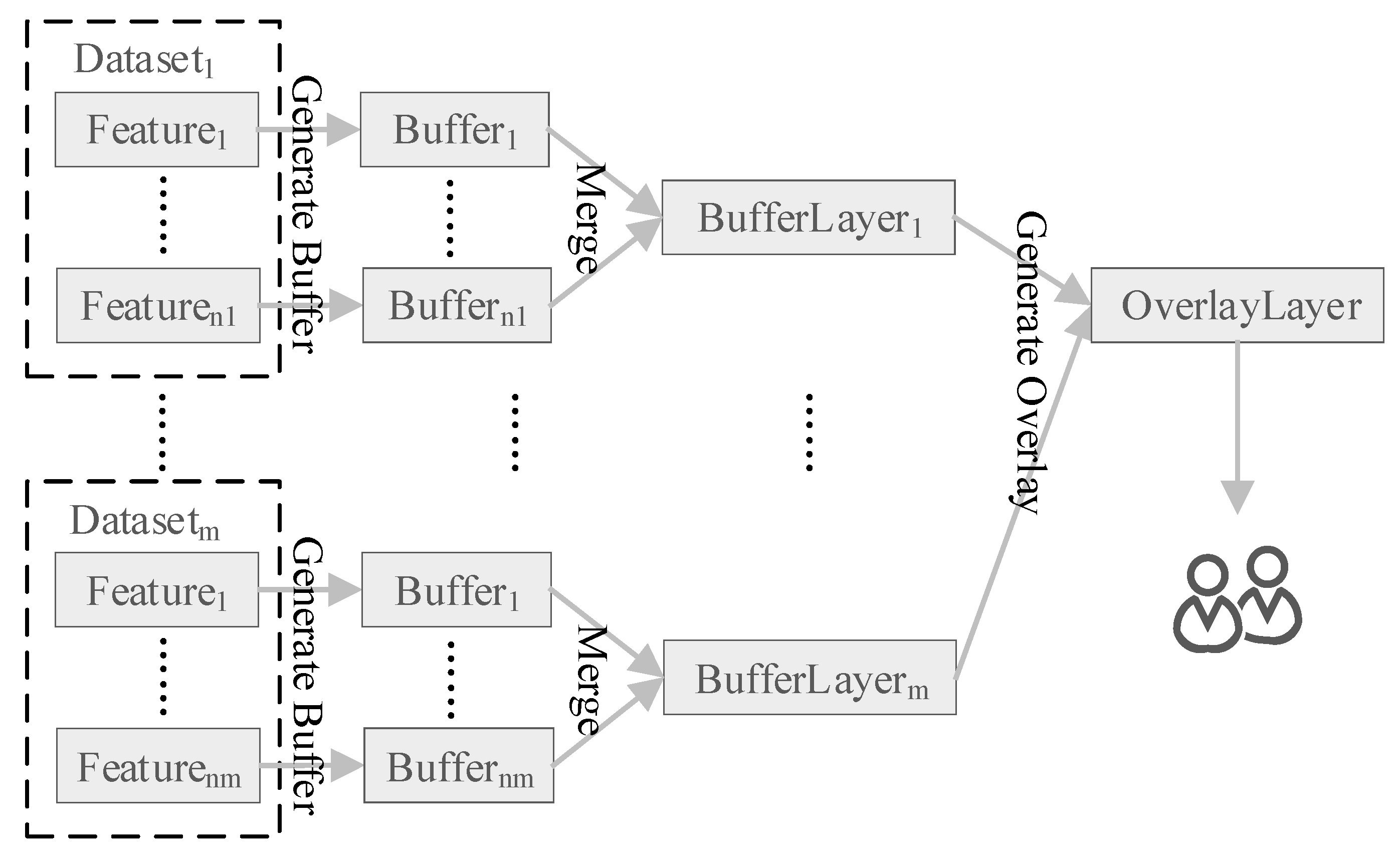
Figure 2 presents the general buffer-overlay analysis flow using existing generation methods. In the flow, buffers of spatial objects are generated separately and merged to create buffer layers of datasets, then the buffer layers are combined to get the final overlay layer. It is data-oriented and straightforward, with computational scales expanding rapidly with the volume of spatial objects. The final overlay layer is provided to users on screens, though it can be extremely large and complex.
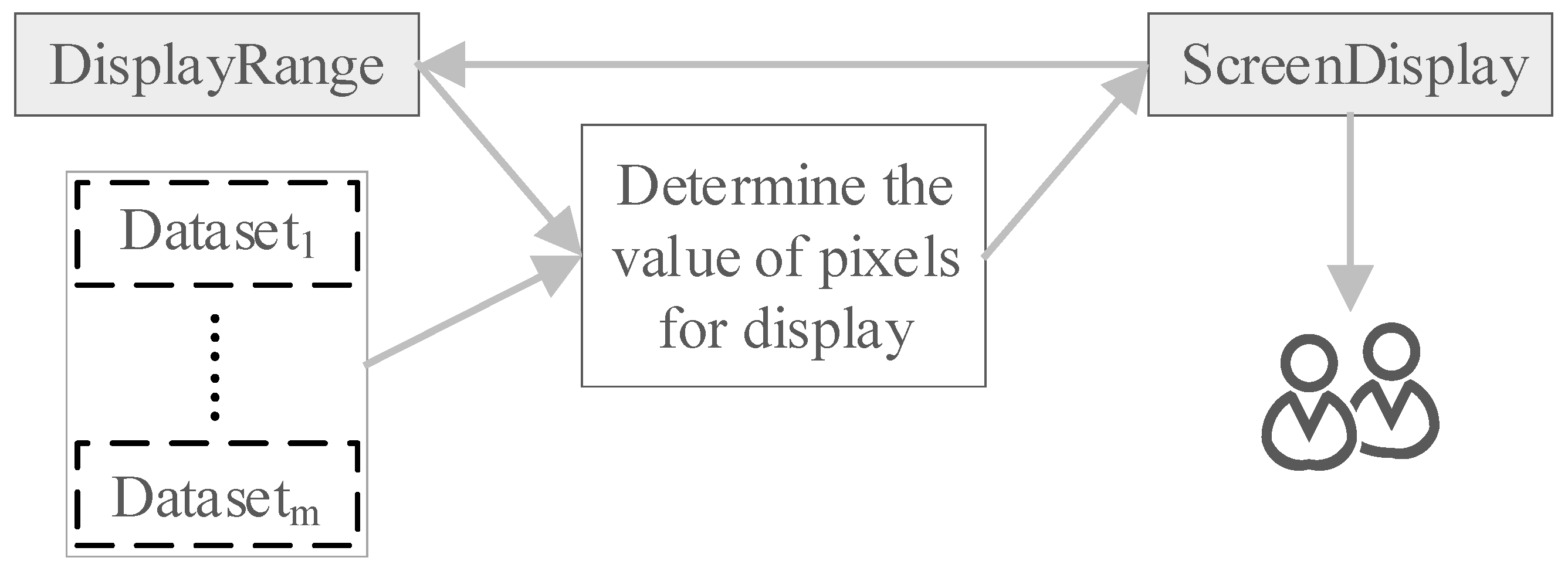
Based on this, we present a visualization-oriented parallel buffer-overlay analysis model, HiBO, to provide interactive and online buffer-overlay analysis of large-scale spatial data. In our previous work, we presented a visualization-oriented buffer analysis method named HiBuffer, which is capable of handling large-scale spatial point and linestring data in real time [21]. Our previous experiments showed that HiBuffer has the striking performance of generating buffers for all of the datasets shown in Table 2 in less than 1 s. In addition, HiBuffer is able to provide interactive buffer analysis for much larger datasets. In this paper, we extend HiBuffer to support buffer analysis of polygon objects and overlay analysis as well, which also achieves remarkable effects. The buffer-overlay analysis flow in HiBO is shown in Figure 3, its core task is to determine the value of pixels for display. To the best of our knowledge, the approach is a brand new idea for buffer and overlay analysis, with the advantage of being insensitive to data volumes. Experimental results verify that HiBO is capable of handling ten-million-scale data in real time.
The remainder of this paper proceeds as follows: Section 2 introduces the core ideas of the buffer and overlay generation methods in HiBO. In Section 3, the architecture of HiBO is described in detail. Section 4 provides an online demonstration, as well as an experiment to validate the performance of HiBO. The conclusions are drawn in Section 5.
2. Methodology
In this section, the core ideas of buffer and overlay generation methods in HiBO will be introduced. In HiBO, we utilize spatial indexes to determine whether a pixel is in the buffers of spatial objects, and accordingly, an efficient buffer generation method named Spatial-Index-Based Buffer Generation (SIBBG) is proposed. Specifically, compared with the SIBBG proposed in our previous work [21], we have extended SIBBG to support polygon objects. As for overlay analysis, HiBO is designed to support complex mixed set operations of multiple buffer analysis results, and we propose the Set-Transformation-Based Overlay Optimization (STBOO) method.
2.1. Spatial-Index-Based Buffer Generation
Spatial indexes are used to optimize spatial queries. As an efficient tree data structure widely used for indexing spatial data, R-tree is implemented by grouping nearby objects and representing them with their Minimum Bounding Rectangle (MBR) in the next higher level of the tree. The spatial queries using R-tree, including bounding-box query and nearest-neighbor search, has been fully optimized theoretically and practically by researchers [22]. In SIBBG, we employ R-tree to determine whether a pixel is in the buffers of spatial objects.
2.1.1. SIBBG for Point and Linestring
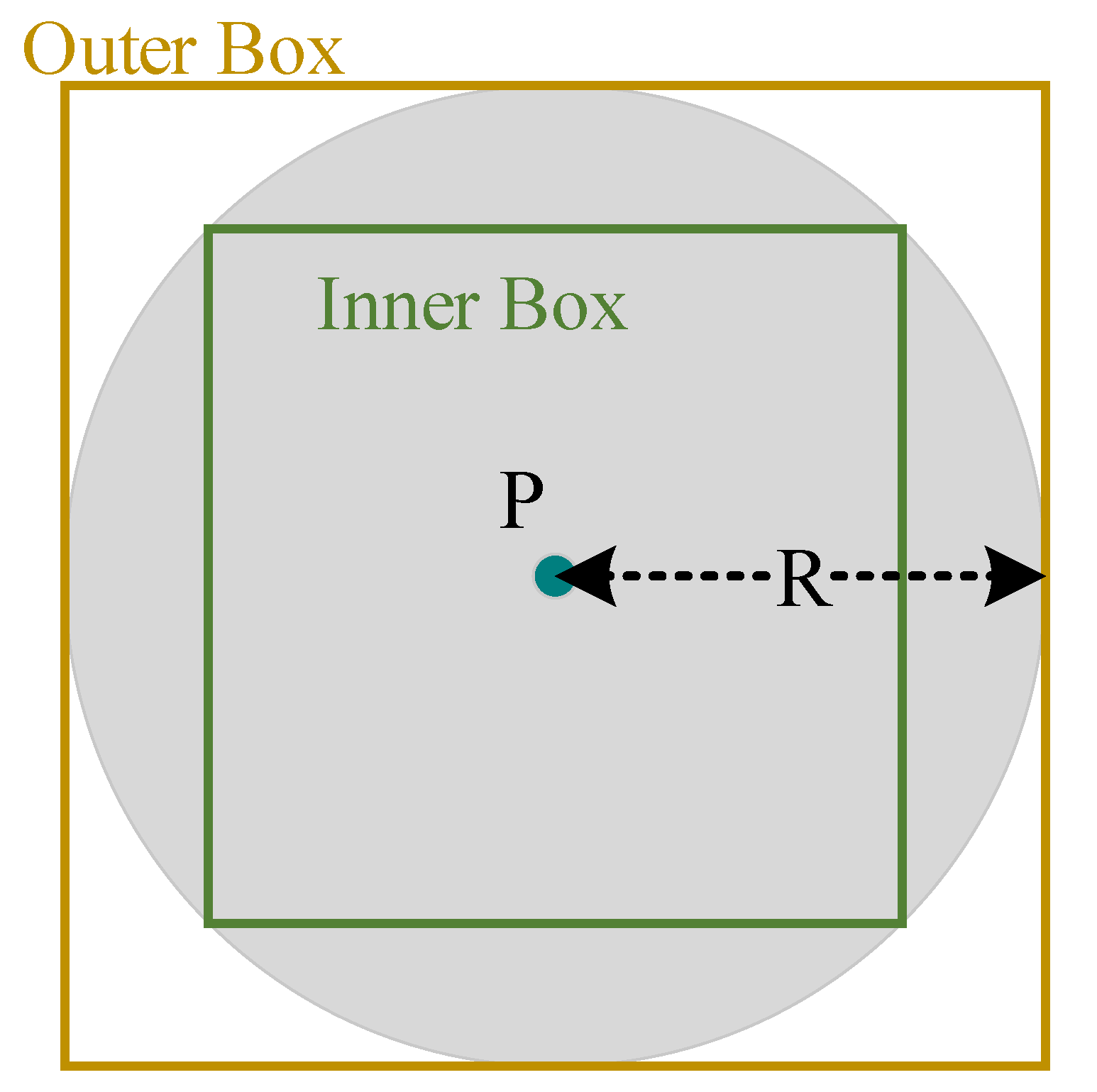
In SIBBG, we utilize R-tree to organize point and linestring objects. Simply, point and segment are used as value types of nodes in R-tree (see Table 3). In R-tree, the intersect operation works well only for a bounding-box query (instead of queries using other polygon shapes), and the nearest-neighbor search has much higher computational complexity than the bounding-box query. Thus, we design SIBBG, as follows, for point and linestring objects (Algorithm 1). In SIBBG, we introduce inner and outer boxes (Figure 4) to optimize spatial queries. As a result of the optimizations, the performance of SIBBG is less sensitive to data volumes.
| Algorithm 1 SIBBG for point and linestring objects [21] |
| Input: Pixel P, radius R, spatial index Rtree. Output: True or False (whether P is in the buffers of spatial objects with a given radius R).
|
2.1.2. SIBBG for Polygon
The buffer generation of polygon objects in HiBO has two issues: The buffer generation of polygon edges, and filling the areas inside polygon objects. As the polygon edges can be treated as linestring objects, we use the same solution adopted for linestring objects. For filling problems, we design a multi-level index architecture to accelerate judging whether a point is inside polygon objects.
As listed in Table 4, we build a two level R-tree for polygon objects. Each polygon edge is stored as a segment in RtreeB; additional node information includes the ID of a given polygon (PolygonID) and whether the edge is parallel to the x-axis (IsLevel). The polygon MBRs are stored as boxes in RtreeMBR. The pseudo-code of SIBBG for Polygon objects is given as follows (Algorithm 2). As shown in line 1–8, for polygon edges we use the same solution adopted for linestring objects. For the areas inside polygon objects, we first use the TmpMBR to find the candidate polygons (line 9) and then judge the spatial relationship between the pixel and each candidate polygon, one by one, until we find the polygon which contains the pixel (line 11–22). We apply the ray-casting algorithm [23] to determine whether a pixel is inside a polygon. To be more specific, given a pixel and a polygon, draw a segment (QuerySegment) from the MBR boundaries of the polygon to the pixel which is parallel to the x-axis, and then use the RtreeB to test how many times the segment intersects the edges of the polygon. The pixel is inside the polygon if the number of crossings is odd, or outside if it is even. The result holds for polygons with inner rings. Moreover, two optimizations (line 10 and line 14–17) have been made to minimize the length of the QuerySegment, as a longer QuerySegment may intersect large numbers of edges which belong to other polygons, and thus cause performance degradation.
| Algorithm 2 SIBBG for polygon objects |
| Input: Pixel P, radius R, spatial indexes RtreeB and RtreeMBR. Output: True or False (whether P is in the buffers of spatial objects with a given radius R).
|
2.2. Set-Transformation-Based Overlay Optimization
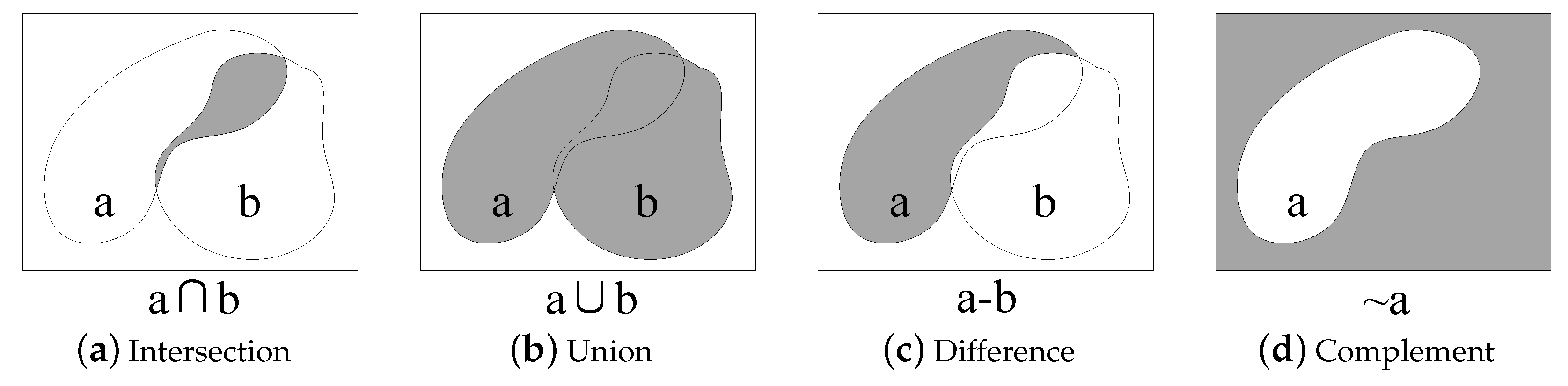
As shown in Figure 5, HiBO supports the four basic set operations on buffer analysis results: Intersection (∩), Union (∪), Difference (−) and Complement (∼). By mixing the operations, most overlay analysis problems can be covered. In STBOO, we reduce computational load by transforming the set operation expressions of overlay analysis. The process of STBOO is as follows.
Step 1 Simplify Expressions
The total computation cost of overlay analysis in HiBO consists of the buffer generation cost and the set operation cost. As illustrated in Equation (1), represents the buffer generation of dataset with radius , is the process of set operation , and C represents the cost.
Table 5 presents the expression simplification of STBOO, which reduces the cost. Take the transformation in the Distributivity Law as an example: Where the expression is transformed from to , the cost changes from to , with the buffer generation and set operation cost both reduced.
Step 2 Reorder Parameters
In HiBO, overlay analysis can be decomposed into tasks of determining the value of each pixel, according to the set operation expressions. The computation cost of a pixel P can be expressed as in Equation (2). represents the process of determining whether P is the buffer of with radius , and is the process of Boolean operation . Compared with SIBBG, the cost of a Boolean operation is much less, and thus BoolCalc is omitted. Accordingly, the computation cost of a pixel P is roughly equal to the sum of SIBBG process costs. As the performance of SIBBG is less sensitive to data size, the optimization target in Step 2 is to reduce the number of SIBBG processes.
According to the Commutativity Law of set operations, for Intersection or Union, reordering parameters will not change the final results. Meanwhile, sometimes the operation results can be determined once the value of the first parameter is calculated, and it is unnecessary to know the value of the second parameter. Typically, if x is false the result of will be false, and if y is true the result of will be true. Thus, the number of SIBBG processes can be reduced by parameter reordering.
The parameter reordering rules of STBOO are listed in Table 6. It should be noted that parameter reordering is only used for the buffer-overlay analysis of point and linestring objects, as polygon objects involve the filling problem and it is hard to estimate the probability of a pixel in the buffers of polygon objects. The rules are simple, efficient, and highly effective. For the Intersection or Union operations of two overlay analysis expressions, we calculate the expression with fewer input dataset layers first (conditions i and ii). For the Intersection operation of two buffer analysis expressions, we calculate the expression with smaller buffer area first (condition iii), as an expression with smaller buffer zone area is more likely to be false. Simply, we assume that a buffer analysis expression with smaller size and radius simultaneously has smaller buffer zone area. And, for the Union operation of two buffer analysis expressions, we calculate the expression with larger buffer area first (condition iv).
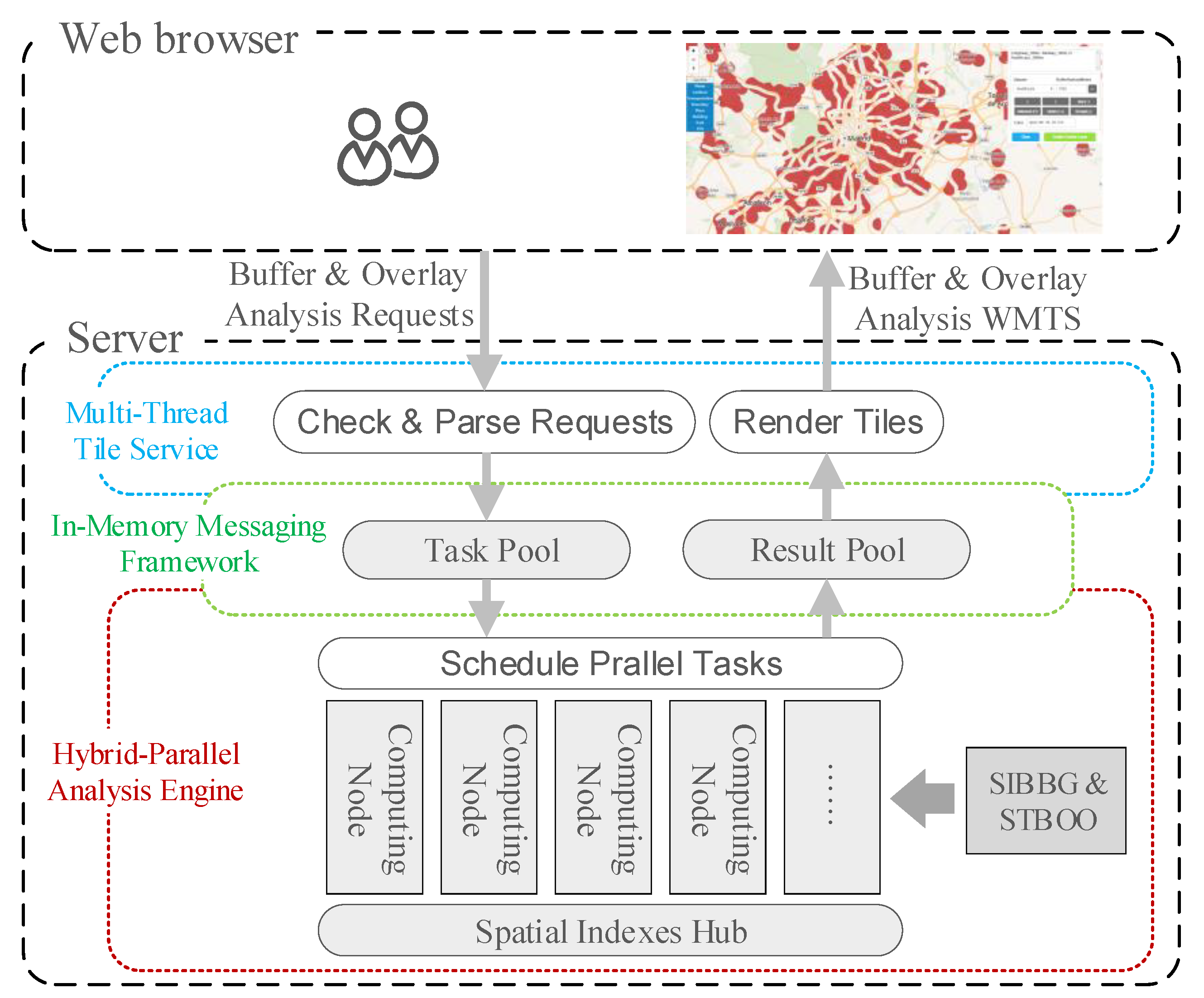
3. Architecture
The architecture of HiBO is illustrated in Figure 6. It adopts the browser-server model. Specially, analysis results are organized into a tile-pyramid structure, provided as a Web Map Tile Service (WMTS). Tiles of different levels are selected for the screen display, according to zoom levels. When a user browses the analysis results, only tiles in the screen range need to be generated. Zooming in the results, tiles with higher levels and higher resolution will be used, and there is no sawtooth distortion. The server side of HiBO comprises three parts: Multi-Thread Tile Service (MTTS), In-Memory Messaging Framework (IMMF), and Hybrid-Parallel Analysis Engine (HPAE).
3.1. Multi-Thread Tile Service
MTTS encapsulates the buffer-overlay analysis service as a WMTS. We treat the analysis task in one tile range as an independent task. In the Check&Parse Requests process, MTTS analyzes the tile requests and filters out improper tasks, including (1) tasks with wrong operation expressions in the requests; and (2) tasks once processed with analysis results are still in the Result Pool. In the Render Tiles process, MTTS gets analysis results from the Result Pool and renders tiles according to the styles in the requests. To be more specific, the analysis results in the Result Pool are stored in the form of two-dimensional boolean arrays (true indicates zones in analysis results). In order to improve concurrency, multi-thread technology is adopted in the tile server.
3.2. In-Memory Messaging Framework
IMMF is a messaging framework based on Redis, which is an In-Memory Key-Value database. In this messaging framework, tasks and results are transferred rapidly in memory without disk I/O. The tasks are stored in a first-in-first-out (FIFO) queue in Redis. Tasks are pushed to the queue and popped to suspended MPI processes. To avoid errors in parallel processing, the push and pop operations are performed in blocking mode. After a task is finished, the analysis result will be written to Redis, and a task completion message will be sent to MTTS using the subscribe/publish functions in Redis. To avoid taking up too much memory, analysis results are set with expiry time, and expired data will be cleaned up once the max memory limit is exceeded.
3.3. Hybrid-Parallel Analysis Engine
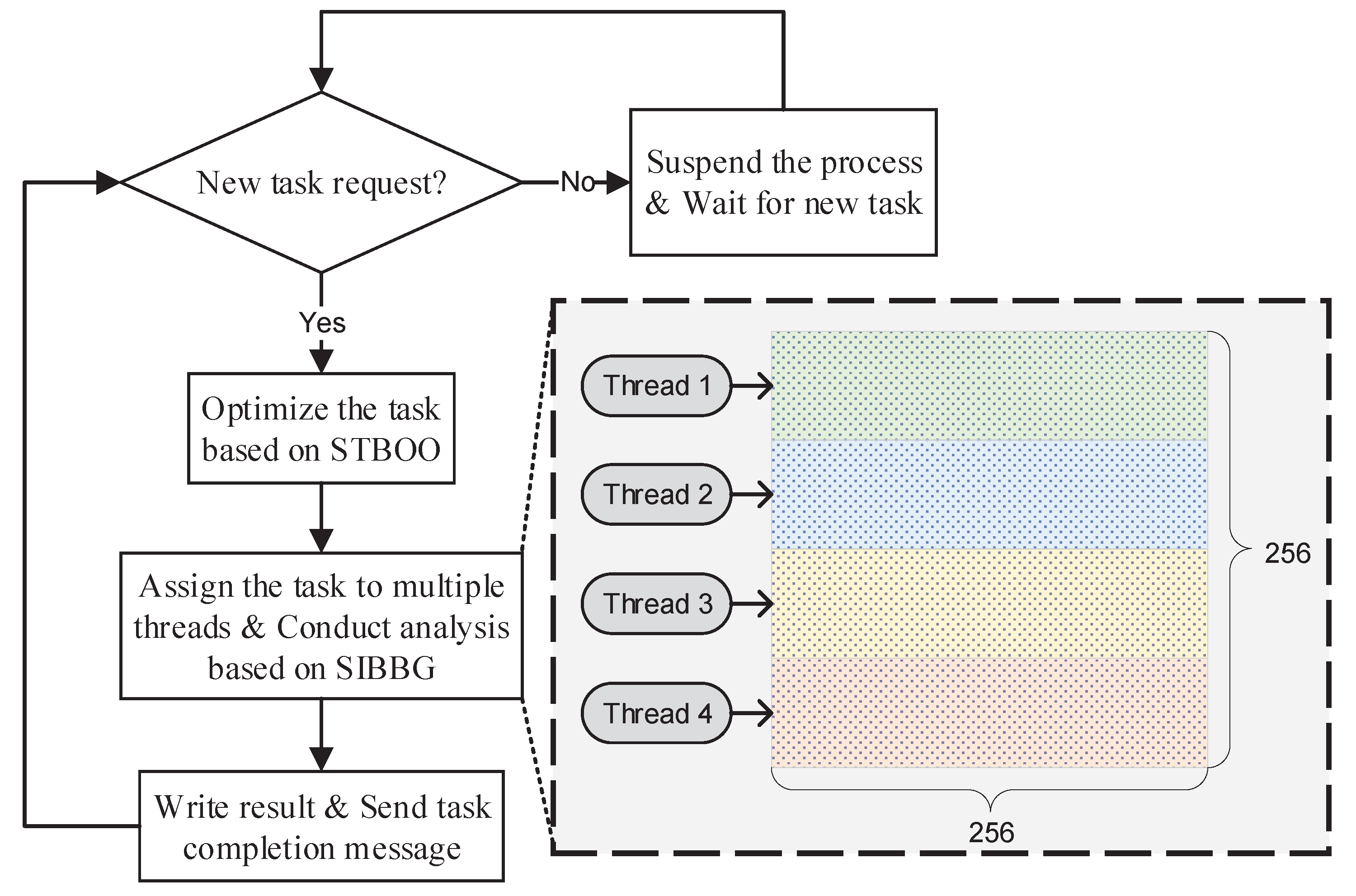
HPAE adopts the hybrid MPI-OpenMP parallel processing model to achieve real-time buffer-overlay analysis. In HiBO, each task is processed with multiple OpenMP threads in one MPI process. As the task requests are generated by way of streaming, the tasks are dynamically allocated to the MPI processes. An MPI process will be suspended after the assigned task is accomplished, and new tasks will be handled on a first in, first served basis. The parallel strategy has the property of good load balancing. An example of the task process is shown in Figure 7.
4. Validation
In this section, we validate the effects of HiBO. First, we provide an online demo, and an application scenario of HiBO is designed. Then, we conduct an experiment to further evaluate the performance of HiBO.
4.1. Setup
The server side of HiBO is implemented using C++ (based on MPICH 3.4), Boost C++ 1.64, and the Geospatial Data Abstraction Library 2.1.2, and the webpage is implemented using JavaScript (based on Mapbox GL 0.49). HiBO is deployed in two high-performance computing environments: An Elastic Compute Service (ECS) server and a Symmetrical Multi-Processing (SMP) server. The hardware environments of the servers are shown in Table 7. The ECS server is used for the online demonstration of HiBO. The SMP server, with more CPU cores and larger memory space, is used to demonstrate the capability of handling large-scale spatial data in HiBO.
4.2. Demonstration
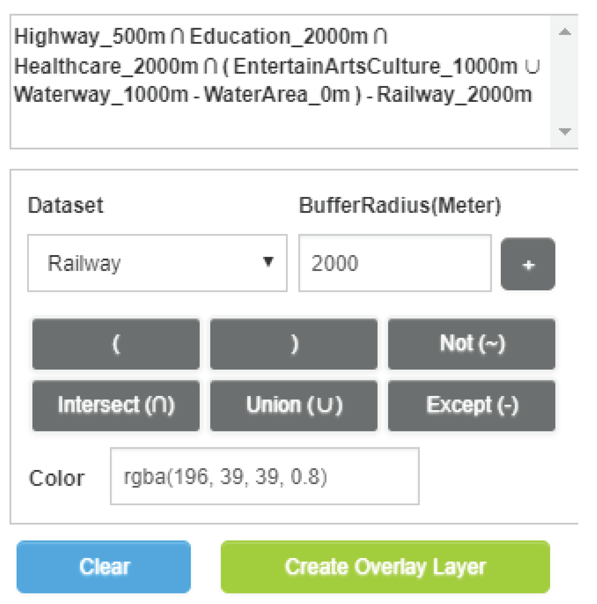
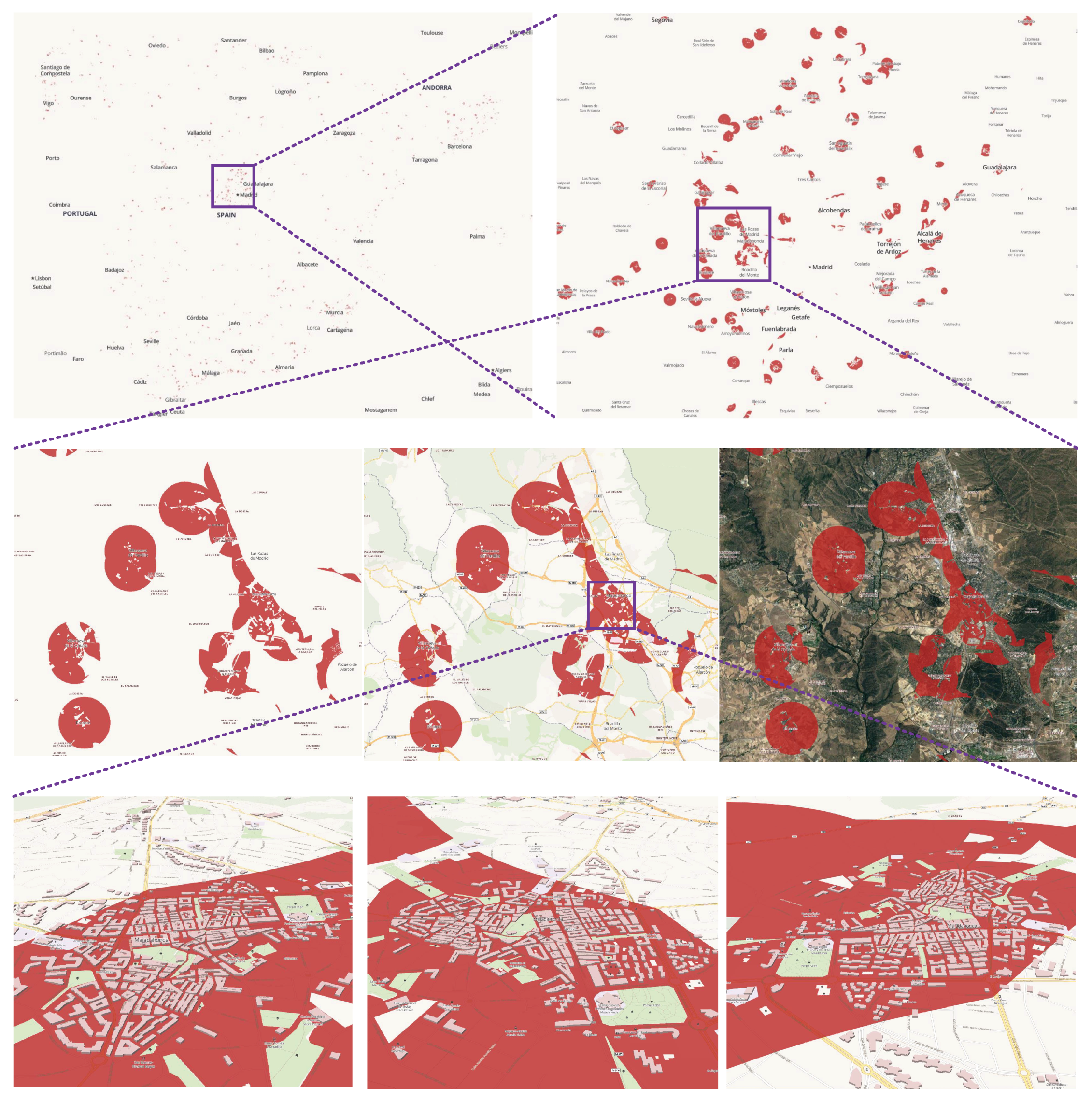
An online demonstration of HiBO is provided on the web (https://github.com/MemoryMmy/HiBO), and we use the datasets of Spain from OpenStreetMap as test data. The demonstration is set to run with 4 MPI processes and 8 OpenMP threads. We have designed a housing site selection scenario to show the effect of the demonstration. The datasets used in the scenario are listed in Table 8. Suppose that a new immigrant in Spain wants to choose a place to live, which meets the following conditions: (1) Convenient to traffic (within 500 m of highways); (2) convenient for children’s education (within 200 m of education amenities); (3) convenient to medical care (within 2000 m of healthcare amenities); (4) near to leisure places (within 1000 m of entertainment, arts & culture amenities, or waterways but not in water area); (5) quiet (at least 300 m away from railways). The conditions can be translated into the following expression (see Equation (3)). Enter the expression into HiBO and click the Create-Overlay-Layer button (Figure 8), and then the result layer will be added to the map in real time. In addition, as the analysis results are preserved in the Result Pool, the color and transparency of the result layer can be adjusted with even faster response. Figure 9 shows the analysis results, in which the red areas are the recommended housing areas for the immigrant.
4.3. Experimental Evaluation
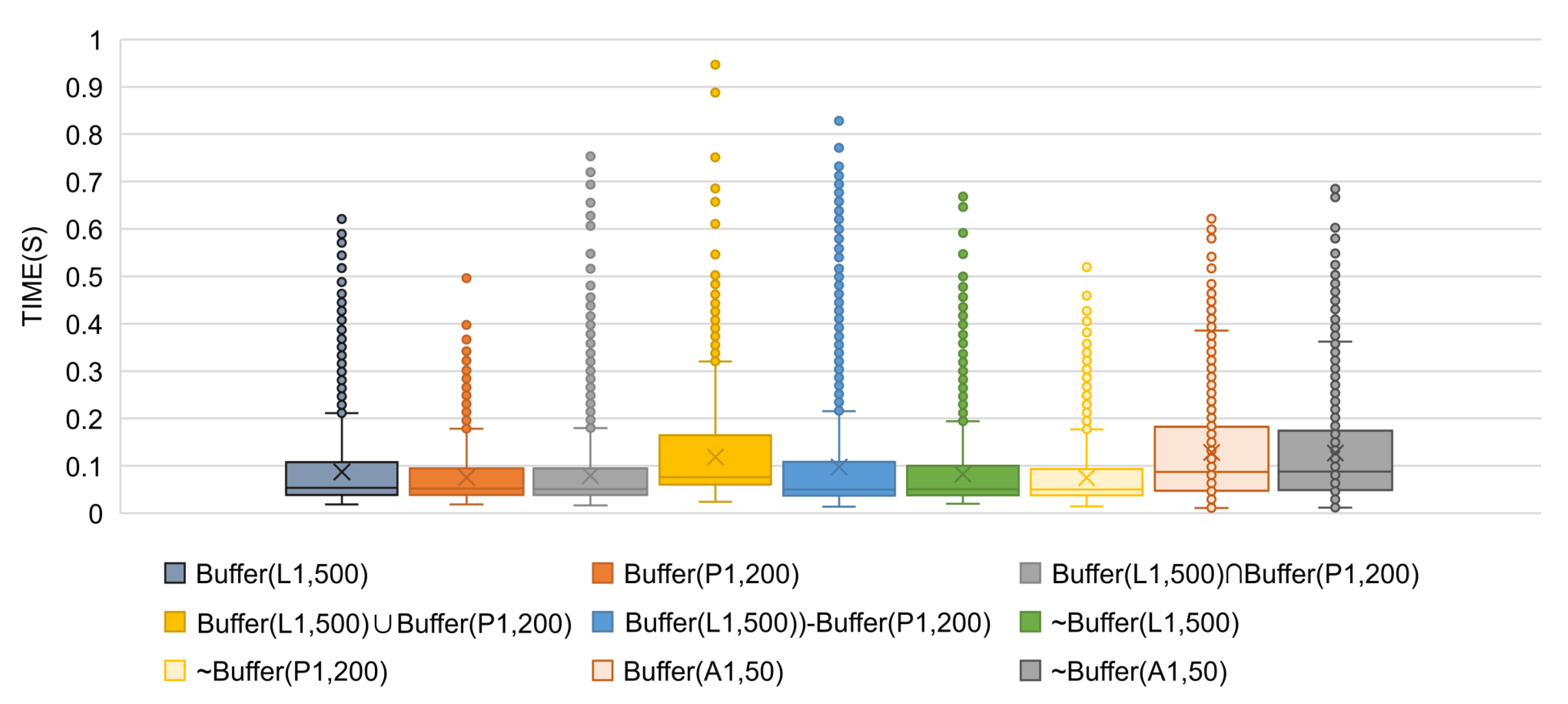
We conduct an experiment on the SMP server to demonstrate the capability of handling ten-million-scale data in HiBO. HiBO is set to run with 32 MPI processes and 2 OpenMP threads in each process. Table 9 shows the datasets used in the experiment. We test the performance of different types of buffer and overlay analysis requests. For each type of request, we generate 5000 tasks, through a test program which randomly requests tiles from different zoom levels. In order to test the performance of analysis engine accurately, HiBO is set to run with no results preserved in the Result Pool. We analyze the tile rendering logs, and the experimental results are shown in Figure 10.
As shown in Figure 10, the tile rendering time distributions of different request types are visualized with box plots (’∘’ represents outliers and ’×’ represents average rendering time). For buffer analysis, datasets of polygon objects produce poorer performance; this is because polygon objects involve the filling process. As illustrated by the figure, the computing time of overlay analysis with two buffer layers as inputs is less than the sum of the generation time of the two buffer layers. This is because of the optimization strategy used in STBOO. Of all request types, produces the poorest performance, though most of the requested tiles are rendered in 0.4 s with the longest rendering time not exceeding 0.7 s. As the number of tiles in a screen range is generally no more than 50, we assume that a browser requests 50 tiles at once. Considering that there are 32 MPI processes, the 50 tasks will be processed in two rounds with 14 (=) MPI processes suspended in the second round—namely, it will be most likely completed in less than 0.8s (= s × 2). In conclusion, HiBO is able to provide interactive and online buffer-overlay analysis of ten-million-scale spatial data.
5. Conclusions and Future Work
This paper presents a parallel processing model, HiBO, for real-time buffer-overlay analysis when the data scale becomes extremely large. Differing from the traditional data-oriented methods, HiBO is visualization-oriented, with the core task transformed into determining the value of pixels for screen display. In HiBO, we employ R-tree to determine whether a pixel is in the buffers of spatial objects, and propose an efficient buffer generation method named SIBBG. HiBO supports complex mixed set operations of multiple buffer analysis results, and we present an effective overlay optimizaation method named STBOO. Parallel computing technologies are used to accelerate analysis in HiBO, and we propose a fully optimized hybrid-parallel processing architecture with good load balancing. Experiments on real-world datasets show that our approach is capable of handling ten-million-scale spatial data. In the future, we will apply our approach to solve the problem of rapid visualization for large-scale vector data.
Author Contributions
M.M. and Y.W. designed and implemented the algorithm; M.M. and L.C. performed the experiments and analyzed the data; J.L. and N.J. contributed to the construction of experimental environment; M.M. developed the visible interface of the demonstration system; M.M. wrote the paper; and Y.W. helped to improve the language expression.
Funding
This research was funded by the National Natural Science Foundation of China under Grant No. 41471321 and No. 41871284.
Conflicts of Interest
The authors declare no conflict of interest.
References
- Sommer, S.; Wade, T. A to Z GIS: An Illustrated Dictionary of Geographic Information Systems; Esri Press: Redlands, CA, USA, 2006; pp. 263–264. [Google Scholar]
- Diamond, J.T.; Wright, J.R. Design of an integrated spatial information system for multiobjective land-use planning. Environ. Plan. B 1988, 15, 205–214. [Google Scholar] [CrossRef]
- Malczewski, J. GIS-based multicriteria decision analysis: A survey of the literature. Int. J. Geogr. Inf. Sci. 2006, 20, 703–726. [Google Scholar] [CrossRef]
- Al-Anbari, M.A.; Thameer, M.Y.; Al-Ansari, N. Landfill Site Selection by Weighted Overlay Technique: Case Study of Al-Kufa, Iraq. Sustainability 2018, 10, 999. [Google Scholar] [CrossRef]
- Peng, H.; Lian, Y.; Chuan-Yong, Y.; Yan-Lan, W. Map Algebra; Wuhan University Press: Wuhan, China, 2006. [Google Scholar]
- Wang, J.; Li, L.I.; Shen, D. Optimization of Boundary Tracing Algorithm on Buffer Generation. Geogr. Geo-Inf. Sci. 2009, 25, 95–98. [Google Scholar]
- Wu, H.; Gong, J.; Li, D. Buffer curve and buffer generation algorithm in aid of edge-constrained triangle network. Acta Geod. Cartogr. Sin. 1999, 28, 355–359. [Google Scholar]
- Li, J.; Qin, Q.; Chen, C.; Zhao, Y.; Xie, C. A method of approximately simulating buffers based on mathematical equations for accelerating buffer analysis. J. Remote Sens. 2013, 17, 1131–1145. [Google Scholar]
- Wang, T.; Zhao, L.; Wang, L.; Chen, L.; Cao, Q. Parallel research and opitmization of buffer algorithm based on equivalent arc partition. Remote Sens. Inf. 2016, 147–152. [Google Scholar]
- Shen, J.; Chen, L.; Wu, Y.; Jing, N. Approach to Accelerating Dissolved Vector Buffer Generation in Distributed In-Memory Cluster Architecture. ISPRS Int. J. Geo-Inf. 2018, 7, 26. [Google Scholar] [CrossRef]
- Wang, Y.; Liu, Z.; Liao, H.; Li, C. Improving the performance of GIS polygon overlay computation with MapReduce for spatial big data processing. Cluster Comput. 2015, 18, 507–516. [Google Scholar] [CrossRef]
- Agarwal, D.; Puri, S.; He, X.; Prasad, S.K.; Shi, X. Crayons—A cloud based parallel framework for GIS overlay operations. Distrib. Mob. Syst. Lab 2011. Available online: https://www.researchgate.net/profile/Hesham_Hefny/publication/309433917_New_Architecture_for_Mobile_GIS_Cloud_Computing/links/5824e6da08aeb45b588f513c/New-Architecture-for-Mobile-GIS-Cloud-Computing.pdf (accessed on 25 October 2018).
- Agarwal, D.; Puri, S.; He, X.; Prasad, S.K. A system for GIS polygonal overlay computation on linux cluster—An experience and performance report. In Proceedings of the 2012 IEEE 26th International Parallel and Distributed Processing Symposium Workshops & PhD Forum, Shanghai, China, 21–25 May 2012; pp. 1433–1439. [Google Scholar]
- Audet, S.; Albertsson, C.; Murase, M.; Asahara, A. Robust and efficient polygon overlay on parallel stream processors. In Proceedings of the 21st ACM SIGSPATIAL International Conference on Advances in Geographic Information Systems, Orlando, FL, USA, 5–8 November 2013; pp. 304–313. [Google Scholar]
- Martinez, F.; Ogayar, C.; Jiménez, J.R.; Rueda, A.J. A simple algorithm for Boolean operations on polygons. Adv. Eng. Softw. 2013, 64, 11–19. [Google Scholar] [CrossRef]
- Puri, S.; Prasad, S.K. A parallel algorithm for clipping polygons with improved bounds and a distributed overlay processing system using mpi. In Proceedings of the 2015 15th IEEE/ACM International Symposium on Cluster, Cloud and Grid Computing (CCGrid), Shenzhen, China, 4–7 May 2015; pp. 576–585. [Google Scholar]
- Puri, S. Efficient Parallel and Distributed Algorithms for GIS Polygon Overlay Processing. Ph.D. Thesis, Georgia State University, Atlanta, GA, USA, 2015. [Google Scholar]
- Apache Spark. 2018. Available online: https://spark.apache.org/ (accessed on 25 October 2018).
- Fan, J.; Ji, M.; Gu, G.; Sun, Y. Optimization approaches to mpi and area merging-based parallel buffer algorithm. Bol. Ciênc. Geod. 2014, 20, 237–256. [Google Scholar] [CrossRef]
- Huang, X. Parallel Buffer Generation Algorithm for GIS. J. Geol. Geosci. 2013, 2, 115. [Google Scholar] [CrossRef]
- Ma, M.; Wu, Y.; Luo, W.; Chen, L.; Li, J.; Jing, N. HiBuffer: Buffer Analysis of 10-Million-Scale Spatial Data in Real Time. Int. J. Geo-Inf. 2018, 7, 467. [Google Scholar] [CrossRef]
- Cheung, K.L.; Fu, A.W.C. Enhanced nearest neighbour search on the R-tree. ACM SIGMOD Rec. 1998, 27, 16–21. [Google Scholar] [CrossRef] [Green Version]
- Shimrat, M. Algorithm 112: Position of point relative to polygon. Commun. ACM 1962, 5, 434. [Google Scholar] [CrossRef]
Figure 1.
Distortion of vector-based and raster-based results while zooming in.

Figure 2.
Buffer-overlay analysis flow using traditional methods.

Figure 3.
Buffer-overlay analysis flow in HiBO.

Figure 4.
Inner and outer boxes of pixel P with a given radius R [21].
Figure 4.
Inner and outer boxes of pixel P with a given radius R [21].

Figure 5.
Set operations of overlay analysis in HiBO.

Figure 6.
Architecture of HiBO.

Figure 7.
Buffer-Overlay analysis of a tile range with pixels in an MPI process with 4 OpenMP threads.
Figure 7.
Buffer-Overlay analysis of a tile range with pixels in an MPI process with 4 OpenMP threads.

Figure 8.
Input of the housing site selection in Spain.

Figure 9.
Analysis result of the housing site selection in Spain.

Figure 10.
Tile rendering time distributions.


Table 1.
Advantages and disadvantages of traditional methods.
| Methods | Advantages | Disadvantages |
|---|---|---|
| Vector-based | (i) Small storage space; (ii) no resolution loss while zooming in. | (i) High computational complexity; (ii) distortion occurs while zooming in (see Figure 1a: In vector polygons, circles or circular-arcs are simplified to regular-polygons or regular-polygon segments). |
| Raster-based | Low computational complexity in overlay generation | (i) Large storage space; (ii) sawtooth distortion while zooming in (see Figure 1b). |
Table 2.
Performance of traditional buffer generation methods.
| Algorithm | 40,927 Linestrings | 208,067 Linestrings | 597,829 Linestrings |
|---|---|---|---|
| HPBM [10] | 10.334 s | 26.859 s | 172.889 s |
| OA1 [19] | 17.041 s | 84.311 s | 672.722 s |
| OA2 [20] | 14.266 s | 280.771 s | 661.857 s |
| OA3 [9] | 19.082 s | 280.8 s | 2534.29 s |
| PostGIS | 34.9 s | 295.8 s | 2380.2 s |
| QGIS | 129 s | 2788 s | >7200 s |
| ArcGIS | 139 s | 2365 s | >7200 s |
| 20.134 s | 200.436 s | >7200 s |
Table 3.
R-tree for point and linestring objects.
| Contents | Value Types |
|---|---|
| Point | point (x,y) |
| Linestring | segment (point (x,y), point (x,y)) |
Table 4.
R-tree for polygon objects.
| Spatial Indexes | Contents | Value Types |
|---|---|---|
| RtreeB | Polygon Boundary | tuple (segment (point (x,y), point (x,y)), PolygonID, IsLevel) |
| RtreeMBR | Polygon MBR | pair (box (point (minx,miny), point (maxx,maxy)), PolygonID) |
Table 5.
Expression Simplification of STBOO.
| Set Laws | Transformation | C | C |
|---|---|---|---|
| Idempotence | Reduced | Reduced | |
| Distributivity | Reduced | Reduced | |
| Reduced | Reduced | ||
| DeMorgan’s laws | Reduced | Reduced | |
| Reduced | Reduced | ||
| Absorption | Reduced | Reduced | |
| Reduced | Reduced | ||
| Complements | Reduced | Reduced | |
| Unchanged | Reduced | ||
| Empty & | Reduced | Reduced | |
| Universal Set | Unchanged | Reduced |
are buffer analysis results; represents universal Set; represents empty Set.
Table 6.
Parameters Reordering of STBOO.
| (i) Condition: |
| (ii) Condition: |
| (iii) Condition: |
| (iv) Condition: |
| Default: Do not reorder parameters. |
D represents dataset of point or linestring objects.
Table 7.
Hardware environments.
| Servers | CPU | Memory |
|---|---|---|
| ECS | 4 cores*2, Intel(R) Xeon(R) [email protected] GHz | 32 GB |
| SMP | 32 cores*2, Intel(R) Xeon(R) [email protected] GHz | 256 GB |
Table 8.
Datasets used in the scenario.
| Dataset | Type | Records | Size |
|---|---|---|---|
| Spain Highway | Linestring | 3,132,496 | 42,497,196 segments |
| Spain Education | Point | 6994 | 6994 points |
| Spain Healthcare | Point | 14,757 | 14,757 points |
| Spain Entertainment, Arts & Culture | Point | 6928 | 6928 points |
| Spain Waterway | Linestring | 33,214 | 4,254,732 segments |
| Spain Water Area | Polygon | 60,319 | 2,044,622 edges |
| Spain Railway | Linestring | 97,675 | 309,716 segments |
Table 9.
Datasets of China.
| Dataset | Abbreviation | Type | Records | Size |
|---|---|---|---|---|
| China roads | L | Linestring | 21,898,508 | 163,171,928 segments |
| China points | P | Point | 20,258,450 | 20,258,450 points |
| China farmland | A | Polygon | 10,520,644 | 133,830,561 edges |
© 2019 by the authors. Licensee MDPI, Basel, Switzerland. This article is an open access article distributed under the terms and conditions of the Creative Commons Attribution (CC BY) license (http://creativecommons.org/licenses/by/4.0/).
Share and Cite
MDPI and ACS Style
Ma, M.; Wu, Y.; Chen, L.; Li, J.; Jing, N. Interactive and Online Buffer-Overlay Analytics of Large-Scale Spatial Data. ISPRS Int. J. Geo-Inf. 2019, 8, 21. https://0-doi-org.brum.beds.ac.uk/10.3390/ijgi8010021
AMA Style
Ma M, Wu Y, Chen L, Li J, Jing N. Interactive and Online Buffer-Overlay Analytics of Large-Scale Spatial Data. ISPRS International Journal of Geo-Information. 2019; 8(1):21. https://0-doi-org.brum.beds.ac.uk/10.3390/ijgi8010021
Chicago/Turabian StyleMa, Mengyu, Ye Wu, Luo Chen, Jun Li, and Ning Jing. 2019. "Interactive and Online Buffer-Overlay Analytics of Large-Scale Spatial Data" ISPRS International Journal of Geo-Information 8, no. 1: 21. https://0-doi-org.brum.beds.ac.uk/10.3390/ijgi8010021
Note that from the first issue of 2016, this journal uses article numbers instead of page numbers. See further details here.